PyAtomDB: Extending the AtomDB Atomic Database to Model New Plasma Processes and Uncertainties

Abstract

The AtomDB project provides models of X-ray and extreme ultraviolet emitting astrophysical spectra for optically thin, hot plasma. We present the new software package, PyAtomDB, which now underpins the entire project, providing access to the underlying database, collisional radiative model calculations, and spectrum generation for a range of models. PyAtomDB is easily extensible, allowing users to build new tools and models for use in analysis packages such as XSPEC. We present two of these, the kappa and ACX models for non-Maxwellian and Charge-Exchange plasmas respectively. In addition, PyAtomDB allows for full open access to the apec code, which underlies all of the AtomDB spectra and has enabled the development of a module for estimating the sensitivity of emission lines and diagnostic line ratios to uncertainties in the underlying atomic data. We present these publicly available tools and results for several X-ray diagnostics of Fe L-shell ions and He-like ions as examples.

1. History of the AtomDB Project

The AtomDB project was originally designed to model X-ray emission from collisionally ionized, optically thin plasma in thermal equilibrium. It built on a history of development, starting with the Raymond–Smith code [1] in 1977 which created spectra for the most abundant 12 elements in a hot plasma using tabulated Gaunt factors and effective collision strengths. In 1985, this was updated by Brickhouse, Raymond, and Smith [2] to improve both the code and atomic data, particularly for the iron L- and K-shell ions. Effective collision strengths were updated and, significantly, the atomic data was separated from the code into independent data files.

In 2001, the first version of AtomDB was released [3]. This included the first release of the publicly accessible atomic database (APED: Astrophysical Plasma Emission Database), complete with defined filetypes as standardized FITS files [4]. In addition, the thermal plasma model, the Astrophysical Plasma Emission Code (APEC), was written and used to convert this database into line and continuum emissivities, which were and are still used extensively in spectral analysis tools such as XSPEC [5] and Sherpa [6]. This was accompanied by another large scale update to the atomic data in APED, in particular for modeling He-like and H-like ions.

In 2012, AtomDB version 2 was released [7]. This again included a large update to atomic data in APED: Ionization and recombination rates were updated, along with new excitation data for He-like and H-like ions. In addition, APED was expanded to include all the elements up to Nickel (previously it had covered only the 14 most abundant elements).

Four years later, AtomDB version 3 was released. This involved a major expansion of the code, the database and tools used to interpret the spectra to allow for the modeling of non-equilibrium ionization plasma, as well as updates to existing atomic data. In particular, there was a need to handle much larger data files (inner shell processes opened up many new levels), calculations for one ion at a time, and new input and output formats suitable for more flexible spectral analysis.

This large scale restructuring of the code exposed inflexibility in the APEC code, which had been designed to run from start to finish and produce one complete output file for the APEC model. To allow for future flexibility, the entire project was shifted to python with the release of the open source PyAtomDB (https://github.com/AtomDB/pyatomdb), which now underpins all aspects of the AtomDB project.

During and subsequent to this, we discovered that new data formats allowed for a significant improvement in AtomDB’s capabilities, enabling a wide range of additional models to be produced. In this paper, we will outline the PyAtomDB project, the new data formats created for non-equilibrium modeling, the new models which this has enabled for charge exchange (CX), non-Maxwellian electrons (Kappa), and the ability to perform uncertainty studies.

1.1. The Astrophysical Plasma Emission Database (APED)

The AtomDB database consists of a selection of data for every ion from H to Ni, all stored as binary FITS (http://fits.gsfc.nasa.gov/fits_standard.html) table files. The data are stored in several different files for each ion, separated by process. Throughout the database, all ions are indexed by their ion charge plus one, so for example He_1 is neutral Helium, and files related to it are stored in the directory $ATOMDB/APED/he/he_1/. There are up to eight different file types for each ion, as listed in Table 1. In addition, APED contains several multi-element files, which hold data covering many ions together, as described in Table 2.

Table 1. File types for per-ion atomic data in the Astrophysical Plasma Emission Database (APED).

Type	Short Description	Details
IR	Ionization & recombination	Ionization from and recombination into the ion.
LV	Energy levels	Energy levels and photoionization cross section data.
LA	Lambda & A-values	Wavelengths and Einstein-A probabilities of transitions.
EC	Electron collisions	Electron-impact excitation rate coefficients or effective
		collision strengths.
PC	Proton collisions	Proton-impact excitation rate coefficients or effective
		collision strengths.
DR	Dielectronic recombination	DR Satellite line wavelengths and intensities.
PI	Photoionization	Photoionization cross sections for ions with data from XSTAR.
AI	Autoionization	Final state selective autoionization transition probabilities.

Table 2. File types for global atomic data in APED. A full description of the data files and formats is included in Appendix A.

Type	Short Description	Details
abund	Elemental abundance	Abundance relative to solar for elements $Z\le 30$
ionbal	Ionization balance	Equilibrium ionization balance and non-equilibrium
		eigenvectors for each element
filemap	List of filenames	The data files used to create the latest release of the
		Astrophysical Plasma Emission Code (APEC) model

Data in the APED is stored as close to the original data format as possible. As a result, there is no single standard for values that are frequently represented as functions, such as collision strengths. Instead there are 10 or more different formats ranging from temperature/value pairs to fit coefficients, each of which can then be interpreted by the APEC code to produce the actual rate coefficient or other value required. This can be confusing for an end user, so part of the motivation for PyAtomDB was to provide a unified interface allowing users to request a piece of atomic data and get the actual rate or coefficient back, instead of the raw fit parameters, etc., which require further interpretation. This accessibility improvement makes using data in other models significantly easier.

1.2. The Astrophysical Plasma Emission Code (APEC)

APEC reads APED and processes the data using a collisional-radiative model to produce line and continuum emissivities on a set temperature and density grid. The plasma is assumed to be optically thin. For each ion at each grid node the excitation rates are calculated and combined with the spontaneous emission coefficients to form a collisional radiative matrix connecting the populations of all levels. Solving this gives level populations through simple multiplication and line emissivities per ion. Ionization and recombination into excited levels is also included in this matrix.

These line emissivities are then multiplied by the elemental abundance (by default [8]), and the ion population in equilibrium to produce the emissivity ${\epsilon }_{ij}$ for each line:

$${\epsilon }_{ij}=A_{ij}{N}_i=A_{ij}\frac{N_i}{N_{z1}}\frac{N_{z1}}{N_Z}\frac{N_Z}{N_H}{N}_H$$

(1)

where $A_{ij}$ is the spontaneous emission coefficient from level i to j, $N_i$ is the number density of ions in excited state i, $N_{z1}$ is the number density of the ion, $N_Z$ is the number density of the element, and $N_H$ is the number density of hydrogen. Therefore these terms from left to right are the spontaneous emission coefficient, the level population, the ion fraction, the elemental abundance relative to hydrogen, and the hydrogen density.

APEC then produces two output files for the plasma, storing two kinds of emissivity data. The line file contains the ${\epsilon }_{ij}$, wavelength, ion and transition identification for each line above a set ${\epsilon }_{ij}$ (by default, ${10}^{-20}$ ph cm³ s⁻¹). The coco files contain the continuum emissivities from bremsstrahlung, radiative recombination and two photon decay, in ph cm³ keV⁻¹ s⁻¹, compressed onto an emissivity vs energy grid by an algorithm [9] which ensures that when the table is linearly interpolated the result is within 1% of the original emissivity value at every point. This is stored on an element by element basis, assuming equilibrium ionization fractions. The coco file also contains the sum of the emission from weak lines not contained in the line file, known as the pseudocontinuum, which is compressed in the same way as the continuum. Within these two files, both of which are standard FITS files, the first Header/Data Unit (HDU) is the list of temperatures, then each subsequent HDU contains the line or continuum emission for one of these temperatures. This data can then be rapidly read by fitting codes such as XSPEC and used to analyze data, interpolating between neighboring temperatures in $log\left(T\right)-log\left(\epsilon \right)$ space.

With AtomDB 3, the introduction of the non-equilibrium ionization (NEI) model means that the ionization fraction, $N_{z1}/NZ$, could not be assumed to be fixed. There are therefore new nei versions of the same data files that do not have this factor included in their emissivity, and for each line and continuum component specify the driving ion which created the feature, as opposed to just the element or ion of the line. For example, the forbidden line of He-like O can originate from the excitation of O⁶⁺, ionization of O⁵⁺, or recombination of O⁷⁺. Creating a model spectrum then involves calculating the ionization fraction for the plasma in question and then multiplying the tabulated emissivities by this to the result to obtain the final emissivity for the model.

1.3. PyAtomDB

The introduction of AtomDB 3 created a vastly larger database to handle all of the underlying atomic processes involved in non-equilibrium processes. In particular, inner-shell excitation and ionization, along with excitation-autoionization, were included in the database for the first time and it was necessary to include ions that are not significant emitters in the X-ray region in equilibrium plasmas, such as M-shell ions.

Initially, APEC was modified to handle these data sets, although it became clear that this was not an efficient method for handling this. The original code started by loading all of the atomic data in the database, then iterating over each temperature, density, element, and ion to produce the spectra. Due to the code’s structure, changing the memory storage alone (required due to the entire database no longer fitting in a reasonable machine’s memory) required a complete re-write of the code. While doing this, it was also converted to Python due to the ease of development, support across different systems, widespread existing use in astronomy, and existing relevant packages such as Astropy [10,11] which PyAtomDB now uses. This conversion enables several long term goals of the project: Users can now run the code themselves, direct access to the APED is possible for those wishing to integrate atomic data lookups into their code, and spectral models based on APED can be developed by users and integrated easily into analysis tools. The resulting six different modules of the PyAtomDB package are listed in Table 3.

Table 3. Modules within PyAtomDB and their purpose. A full description is provided in the code documentation (https://atomdb.readthedocs.io).

Module	Purpose
atomdb	Accessing the database, returning atomic data
apec	Thermal plasma model
spectrum	Creating spectra from apec outputs
atomic	Basic atomic data (element names, etc.)
const	Physical and code related constants
util	Utilities and helper routines

A full manual of the capabilities of PyAtomDB is beyond the scope of this paper. We will instead highlight some of the capabilities of the spectrum module, creating spectra of interest to end users, and extensions to it for modeling different, non-standard plasma types and investigating the effects of uncertainties on atomic data.

2. Spectral Modeling with PyAtomDB

The spectrum module in PyAtomDB contains routines for creating collisional ionization equilibrium (CIE) spectra of thermal plasmas, complete with applying instrument responses. These tools are also provided with wrappers, allowing them to be used in PyXspec (https://heasarc.gsfc.nasa.gov/xanadu/xspec/python/html/).

2.1. Non-Equilibrium Ionization Modeling

In addition to simple CIE plasmas, there are extensive models for NEI plasmas within PyAtomDB. These models represent a plasma where the electron temperature has rapidly changed, however the charge state distribution of the ions has not yet had time to reach a new equilibrium at this temperature. As the timescale for ionization and recombination is significantly longer than that for individual level populations to change, there is significant emission from ions at temperatures where they would not normally be observed in CIE. Such plasmas can be found in any place with shock heating—for example young Supernova Remnants (SNR) where the reverse shock rapidly heats the electrons leaving the plasma in an ionizing state until the plasma reaches equilibrium again e.g., [12]. Similarly, a recombining plasma, where the electrons have undergone a rapid cooling, can be found in many Mixed Morphology SNR, where rapid expansion leads to rapid cooling of the electrons and a subsequent recombination dominated plasma [13].

Figure 1 shows an equilibrium, ionizing from $k{T}_e=0.07$ keV and recombining from $k{T}_e=7.0$ keV spectrum for a $k{T}_e=0.7$ keV plasma at an ionization timescale of ${10}^{10}$ cm⁻³s. The ionizing case is dominated by He-like lines of Si and Ne, while the recombining case shows significant emission from He- and H-like Fe, as well as the H-like Si and Mg ions.

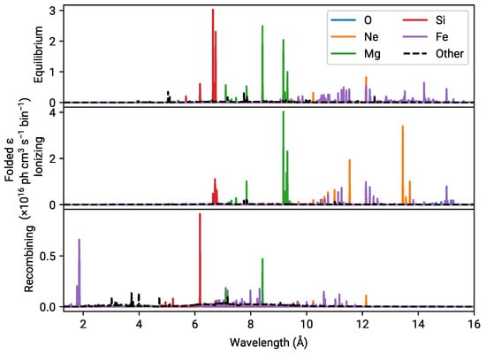
Figure 1. Emission from $k{T}_e=0.7$ keV plasmas in equilibrium, ionizing (from $k{T}_e=0.07$ keV) and recombining (from $k{T}_e=7.0$ keV). The ionization timescale is $n_{e}t={10}^{10}$ cm⁻³ s for both non-equilibrium cases. Spectra have been folded though the Chandra ACIS-S/HETG +1 order response from Cycle 22.

This model is identical to the existing rnei model in XSPEC, but has additional flexibility such as allowing the user to identify strong lines in a selected wavelength region of a non-equilibrium plasma. There is a similar model for a plane-parallel shock (pshock) [12].

2.2. Non-Maxwellian Modeling

Non-Maxwell–Boltzmann electron energy distributions can occur in a range of astrophysical plasmas such as the Earth’s magnetosphere [14], supernova shock waves (e.g., [15]), or solar flares (e.g., [16]). In these cases, the electron energy distribution is not well represented by a Maxwellian distribution due to an excess of high energy electrons. These can be modeled by a $\kappa$ distribution:

$$f_{\kappa }\left(E;\kappa ,T\right)=A_{\kappa }\frac{2}{\sqrt{\pi }}{\left(\frac{1}{k_{B}T}\right)}^{\frac{3}{2}}\sqrt{E}{\left[1+\frac{E}{\left(\kappa -\frac{3}{2}\right)k_{B}T}\right]}^{-\left(\kappa +1\right)}$$

(2)

where:

$$A_{\kappa }=\frac{\Gamma (\kappa +1)}{\Gamma \left(\kappa -\frac{1}{2}\right){\left(\kappa -\frac{3}{2}\right)}^{\frac{3}{2}}}.$$

(3)

When $\kappa$ approaches its lower limit of 3/2, the distribution is highly non-Maxwellian, when $\kappa =\infty$ it is once again Maxwellian.

Most electron energy dependent atomic data is, however, collated assuming the electron energies follow a Maxwellian distribution, as it saves substantial disk space, speeds computation of emissivities, and is relevant to the majority of applications. In theory the parameters such as electron collision strengths could be recalculated from first principles for non-Maxwellian plasmas, however the underlying cross section data either no longer exists for the vast majority of ions or, if they are, are too unwieldy for practical use. As a result, representing the $\kappa$ distribution as a sum of Maxwellian plasmas presents an attractive compromise. We have implemented [17] the decomposition method of [18] to create spectra for non-Maxwellian plasma, wherein several different Maxwellian temperatures are added to closely approximate a true $\kappa$ energy distribution.

Initially this was to be performed as a complete rewrite of the underlying model, however with the flexibility of PyAtomDB and the new data formats, we are able to achieve this using a simple 2-step process: The effective ionization and recombination rates are calculated by appropriately summing the Maxwellian rates as shown in Figure 2, the charge state distribution is calculated, and then the non-equilibrium emissivities can be combined with these to provide a non-Maxwellian spectrum.

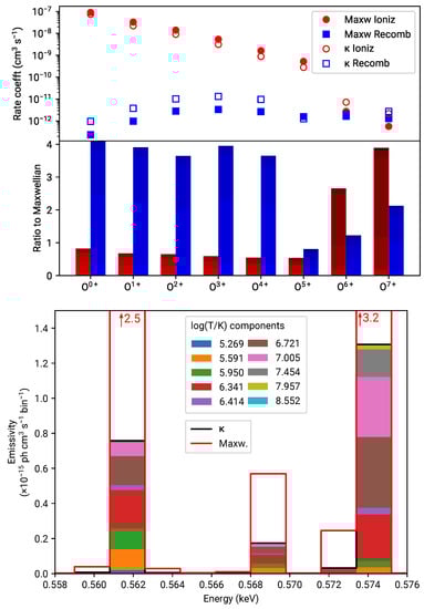
Figure 2. Ionization and recombination rate coefficients of oxygen in a kT = 0.2 keV, $\kappa$ = 2.0 plasma. Top: The total rate coefficients for the $\kappa$ and Maxwellian case. Middle: The ratio of the $\kappa =2.0$ ionization (red) and recombination (blue) rates to their Maxwellian equivalent. The different shades represents the contribution of each Maxwellian component from the decomposition method of [18]. Bottom: The resulting emission in the O⁶⁺ He-$\alpha$ triplet. The components of the Maxwellian decomposition are again shown in different colors. Note that the Maxwellian total emissivity, marked with the red line, is larger due to the charge state distribution having more O⁶⁺ in the Maxwellian case.

2.3. Charge Exchange

Charge exchange occurs when a donor ion or atom with one or more electron still attached interacts with a recombining ion, which is missing at least one electron, resulting in the transfer of the electron from the donor to the receiver:

$$R^{y+}+D^{z+}\to R^{(y-1)+}+D^{(z+1)+}$$

(4)

where R is the recombining ion, and D is the donor. In most situations where charge exchange is postulated (e.g., the solar wind), the donor is neutral hydrogen as the only element with a significant enough abundance for the interaction to be observable. Typically, the exchanged electron is captured into an excited state of the ion, and these are often significantly higher n and l shells than those populated by electron impact excitation. As the ion relaxes to its ground state, the line emission is therefore significantly different from that observed in a typical thermal plasma. In some cases this can allow for the direct identification of CX, but in many more cases the foreground CX emissions adds an additional nuisance component to the spectrum of interest.

We released version 1 of the AtomDB Charge Exchange (ACX) model in 2014. This used a combination of analytical nl shell capture distribution formulae with a cascade to ground calculated through the APED database to create spectra useful for identifying CX emission [19], and successfully used it to model the spectrum of the hot and cool solar wind components.

However, the model had several shortcomings. On the physics side, the CX process was modeled without any velocity dependence, with the user selecting from one of four analytical cross section models to see which worked best. On the implementation side, the model relied on a computationally expensive process combining the AtomDB database to produce the spectra and line lists of interest. This meant that as the APED database was updated in the future, the changes in line wavelength and A-values were not reflected in the ACX model.

To expand the model, for ACX version 2 theoretical charge exchange cross sections (as opposed to the analytical $nl$ distributions), including velocity dependent effects, were obtained from the Kronos database [20,21,22]. PyAtomDB was then used to create spectra for capture into each $nl$ shell, and subsequent cascade to the ground state. By treating each of these as independent spectra, as if they were separate ions in the NEI model, spectra can be rapidly created in two steps: First, the cross section for capture into each $nl$ shell is calculated, then the spectrum for each $nl$ shell is multiplied by this cross section and then summed:

$${\epsilon }_{CX}=\sum ^{nl}{\sigma }_{nl}\left(E\right)v{\epsilon }_{nl}$$

(5)

where ${\epsilon }_{CX}$ is the total CX emissivity, $nl$ is the shell captured into, E and v are the energy and velocity of the center of mass of the donor-recombining ion, and ${\epsilon }_{nl}$ is the emissivity for capture into that one specific $nl$.

2.4. Cross Section Data Selection

The Kronos database contains only nlS selective cross sections for collisions with a hydrogen donor and a H-like recombining ion, and also for the bare recombining ion of C, N, O, and Ne. For all other bare ions, and for He as the donor, data is only resolved to the n shell.

In the case of nlS resolved data, the total capture into all the states which match the nlS is split evenly. For n resolved data the l shell distribution is handled by one of the analytical distribution functions described for ACX version 1 (the user may choose which one). For all other ions, where there is no data in the Kronos database, the model falls back to the ACX 1 models, with the total cross section fixed at $3\times {10}^{-15}$ cm².

Within the Kronos database, there are often different data sets present for the same ion. As the authors of the database themselves advised, we choose the data which exists from the best available technique if no specific set is recommended. The techniques are ranked from quantum molecular orbital close coupling (QMOCC) [23], atomic orbital close coupling (AOCC) [24], classical trajectory monte carlo (CTMC) [25,26], to multi-channel Landau Zener (MCLZ) [27].

2.5. Spectral Generation

For each nl or nlS to which capture is possible given the cross section in the Kronos database, we calculate the spectrum by creating a radiative matrix assuming no further collisional excitation as the electron cascades to the ground state. The A-values are taken from the AtomDB database for all ions where they exist.

For some heavier ions, the n shell for capture ends up being very high, e.g., 16 for the donor Fe²⁵⁺. This is beyond the AtomDB holdings, which stop at $n=10$ for He- and H-like ions and at $n\le$ 7 for all other ions. For these cases we have topped up the existing AtomDB A-values and wavelengths using calculations from Autostructure [28]. Where possible, the wavelengths for these calculations have been shifted to match the NIST ASD [29] values. The new energy levels were matched to the existing AtomDB levels using energy-order, symmetry, and degeneracy matching. For the Li-, He-, and H- like ions these matches were relatively trivial, though in the middle of the Fe L shell ions this matching becomes more problematic. Fortunately, the inaccuracies introduced by poor wavelengths at high energies in these complex ions can be largely discounted due to the fact that the sheer number of lines prevents any one line from producing a strong spectral signature. By contrast, a simple ion such as O⁷⁺ has a straightforward series of lines with well established wavelengths, and therefore discrepancies would be more pronounced.

Constructing the model in PyAtomDB has two distinct advantages: It allows the model to be rapidly developed (as it reuses most of the tools for NEI plasma) and it enables users to deploy it using the same commands.

3. Estimating the Impact of Uncertainties with PyAtomDB

Varying Atomic Data

Estimating the magnitude of the uncertainties on rates for fundamental atomic processes is a difficult task with no obvious correct solution. The source data comes from a wide range of theoretical and experimental sources, often lacking sufficient information on the associated uncertainties to make a meaningful estimate. Nevertheless, there is significant effort being applied to estimating atomic data uncertainties: Most atomic data publications in the past decade have some effort to make reasonable uncertainty assessments, and there are several groups e.g., [30,31] that are working on trying to estimate uncertainties on the existing atomic data.

Given the magnitude of this task, being able to direct the efforts by identifying the atomic data which line emission and ratio diagnostics are most sensitive to is essential for more accurate data analysis. We have developed the variableapec (https://github.com/AtomDB/variableapec) module, which makes use of routines in PyAtomDB to identify which atomic processes most strongly affect the resulting spectra. The user can vary any fundamental atomic data in the AtomDB database by a set amount and re-run emissivity calculations to identify which lines are sensitive to the changed parameter. This allows users to investigate the sensitivity of line and line ratio emissivities over a range of temperatures and densities. The module also checks for other lines affected from perturbing a single line.

Varying an atomic rate of a single transition may have cascading effects for other transitions, depending on the strength of the line varied or the levels of the transition. The user can input a range of wavelengths and cutoff threshold for the fractional emissivity change and plot lines sensitive to the transitions changed. This is an important diagnostic of lines that are sensitive to cascade effects as well as a diagnostic of correlated errors. Throughout this work we provide errors as the mean value of the positive and negative uncertainties for the fractional emissivity change. Line ratio errors are half the range of the maximum and minimum ratios obtained when applying both positive and negative uncertainties to the individual atomic data.

Figure 3 shows Fe xvii lines sensitive in the range of 10–20 Å to a ±30% change in A value in key emission lines at low density and the temperature where Fe xvii peaks in abundance. Varying the A value for the 3E transition alone resulted in a greater than 0.01% change in emissivity for not only the 3E transition but also four other lines in the range of 10–20 Å. Note that at a low density, the emissivities of the lines are almost only sensitive to the rate of population into the level (i.e., the effective collision strengths) as opposed to the rate out (i.e., the A values). 3E also has the greatest fractional change in emissivity of the six key transitions with A values perturbed by 30%. The value of 30% chosen for the uncertainty on the A-value is deliberately large for demonstration purposes, although it is in line with the uncertainties on the 3C and 3D line ratios reported in Bernitt et al. [32], and NIST Atomic Spectral Database uncertainties for these lines are class C ($\pm 18\%$) and D ($\pm 50\%$).

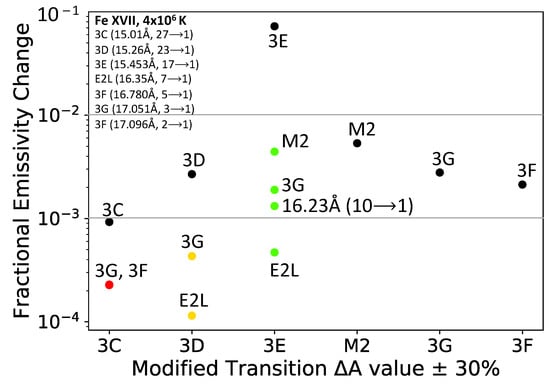
Figure 3. Fe xvii emission lines in the range of 10–20 Å sensitive to a ±30% change in A value at $T_e=4\times {10}^6$ K and low density. Black points denote the emissivity change for the transition varied while colored points denote other transitions affected for each perturbed line.

The new variability module also allows the user to vary the atomic rates of two separate transitions and recalculate diagnostics for that line ratio, such as the Fe xvii 3C/3D ratio shown in Figure 4. Line ratios can be sensitive to either temperature or density, making them useful diagnostics of estimating a plasma’s temperature or density. It is more informative to add uncertainties to two lines individually and recalculate line ratios rather than adding a blanket uncertainty to the final line ratio.

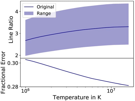
Figure 4. Fe xvii 3C/3D line ratio at low density as a function of temperature with a ±15% uncertainty on the direct excitation rates of both the 3C and 3D lines. The final error on the line ratio is ∼30% for the entire temperature range plotted.

variableapec can also apply uncertainties for more complicated line ratios, such as the G and R ratios in the $n=2\to 1$ transition lines of He-like ions [33]. These are the ratios of the forbidden plus intercombination lines to the resonance lines (G) and the forbidden to intercombination (R) lines, which are temperature and density dependent respectively. It adds the same uncertainty to the forbidden, intercombination, and resonance lines and then calculates the error propagation on the individual rate changes to produce an error on the final line ratio. Figure 5 and Figure 6 show the effect of perturbing these key emission lines for the O vii R ratio and Fe xxv G ratio respectively. We applied a constant error over a temperature or density range, however the errors on the underlying data can be significantly temperature dependent, e.g., effective collision strengths. Future steps include recalculating line emissivities and line ratios with representative temperature-dependent errors.

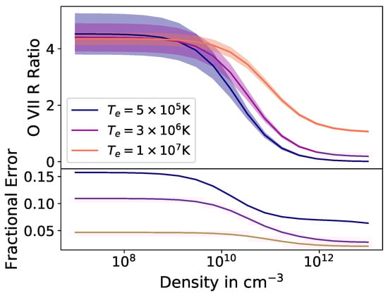
Figure 5. O vii R ratio with a ±15% uncertainty on the direct excitation rates of the forbidden, resonance, and intercombination lines at three different plasma temperatures.

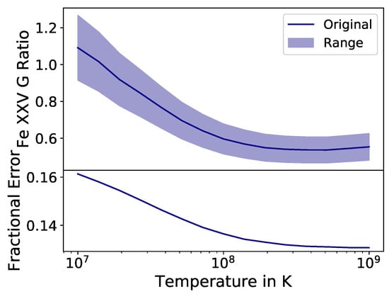
Figure 6. Fe xxv G ratio with a ±15% uncertainty on the direct excitation rates of the forbidden, resonance, and intercombination lines at low density. The final error on the line ratio is ∼15% for the entire temperature range plotted.

The tool allows the user to recalculate line diagnostics at multiple temperatures or densities. It is informative to estimate the fractional error on the resulting line ratio after varying the A value or direct excitation rate of a density- or temperature-sensitive line. The O vii R ratio at three different plasma temperatures in Figure 5 shows that the magnitude of fractional error varies for different plasmas.

When a pair of lines is blended, it is more useful to add the uncertainty onto the three lines individually and recalculate the blended line ratio. Figure 7 shows the blended line ratio of (209.62 + 209.92) Å/213.77 Å for Fe xiii, a density-sensitive line ratio often used in solar physics [34].

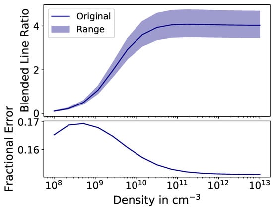
Figure 7. Blended Fe xiii line ratio (209.62 + 209.92) Å/213.77 Å versus density at Te = 200 eV. The final error on the line ratio is ∼16% for the entire temperature range plotted.

4. Summary

The new PyAtomDB package had been released as open source code. It is now possible for the astronomy community to obtain all of the data, thermal plasma codes, and spectral models based on the project, and to develop extensions based on it.

We have developed modules for charge exchange and non-Maxwellian electrons, which are compatible with PyAtomDB and analysis tools such as PyXspec. The code can easily be extended to include new models the community may contribute.

In addition, we have used the newly available codes to develop a tool for estimating the sensitivity of spectral diagnostics to uncertainties in the underlying atomic data, which is immediately applicable to a range of plasmas for upcoming high resolution missions such as XRISM.

Appendix A.1. Ion-by-Ion Files

Table A1. APED IR (ionization and recombination rate) file definition. Excluded data types (XI, XR, and XD) are used to populate excited levels of ions but are not used when calculating the charge state distribution. The effect of these rates is included in the CI, EA, DR, and RR total rates used for calculating the charge state distribution. Notable header keywords: IONPOT contains the ionization potential in eV.

Name	Format	Description
Element	1J	Atomic Number
Ion_init	1J	z1 of initial ion
Ion_final	1J	z1 of final ion
Level_init	1J	level process starts in
Level_final	1J	level process finished at
TR_Type	2A	Transition type. One of:
		CI : Collisional Ionization
		EA : Excitation Autoionization
		XI : eXcluded Ionization
		DR : Dielectronic Recombination
		RR : Radiative Recombination
		XR : eXcluded Radiative recombination
		XD : eXcluded Dielectronic recombination
TR_Index	1J	Line index in file (starting from 1)
Par_Type	1J	Parameter type. Defines meaning of Temperature and IonRec_Par
		51: CI: Coefficients from Younger [35].
		61: EA: Lithium coefficients from Arnaud & Rothenflug [36].
		62: EA: Other coefficients from Arnaud & Rothenflug [36].
		63: EA: Coefficients from Mazzotta [37].
		71: RR: Coefficients from Shull & Van Steenberg [38].
		72: RR: Coefficients from Verner & Ferland [39].
		73: RR: Coefficients from Arnaud & Raymond [40].
		74: RR: Coefficients from Badnell [41].
		81: DR: Coefficients from Mazzotta [37].
		82: DR: Coefficients from Badnell [42].
		100: CI: Coefficients from Dere [43].
		Interpolatable arrays of N Rate Coefficients (cm3 s−1):
		300+N: include both left and right boundary
		350+N: include neither boundary
		700+N: include only minimum boundary
		750+N: include only maximum boundary
		900+N: CI: Interpolatable array of N ${\rm Y}$ effective ionization coefficients.
Min_Temp	1E	Minimum Temperature for which data is valid (K)
Max_Temp	1E	Maximum Temperature for which data is valid (K)
Temperature	20E	Array of up to 20 temperatures (K)
IonRec_Par	20E	Array of up to 20 rate coefficients (cm3 s−1)
		or coefficients as Par_Type indicates.
Wavelen	1E	Deprecated
Wave_Obs	1E	Deprecated
Wave_Err	1E	Deprecated
BR_Ratio	1E	Deprecated
BR_Rat_Err	1E	Deprecated
Label	20A	Deprecated
Rate_Ref	20A	Bibcode of reference for rates
Wave_Ref	20A	Deprecated
Wv_Obs_Ref	20A	Deprecated
Br_Rat_Ref	20A	Deprecated

Table A1. APED IR (ionization and recombination rate) file definition. Excluded data types (XI, XR, and XD) are used to populate excited levels of ions but are not used when calculating the charge state distribution. The effect of these rates is included in the CI, EA, DR, and RR total rates used for calculating the charge state distribution. Notable header keywords: IONPOT contains the ionization potential in eV.

Name	Format	Description
Element	1J	Atomic Number
Ion_init	1J	z1 of initial ion
Ion_final	1J	z1 of final ion
Level_init	1J	level process starts in
Level_final	1J	level process finished at
TR_Type	2A	Transition type. One of:
		CI : Collisional Ionization
		EA : Excitation Autoionization
		XI : eXcluded Ionization
		DR : Dielectronic Recombination
		RR : Radiative Recombination
		XR : eXcluded Radiative recombination
		XD : eXcluded Dielectronic recombination
TR_Index	1J	Line index in file (starting from 1)
Par_Type	1J	Parameter type. Defines meaning of Temperature and IonRec_Par
		51: CI: Coefficients from Younger [35].
		61: EA: Lithium coefficients from Arnaud & Rothenflug [36].
		62: EA: Other coefficients from Arnaud & Rothenflug [36].
		63: EA: Coefficients from Mazzotta [37].
		71: RR: Coefficients from Shull & Van Steenberg [38].
		72: RR: Coefficients from Verner & Ferland [39].
		73: RR: Coefficients from Arnaud & Raymond [40].
		74: RR: Coefficients from Badnell [41].
		81: DR: Coefficients from Mazzotta [37].
		82: DR: Coefficients from Badnell [42].
		100: CI: Coefficients from Dere [43].
		Interpolatable arrays of N Rate Coefficients (cm3 s−1):
		300+N: include both left and right boundary
		350+N: include neither boundary
		700+N: include only minimum boundary
		750+N: include only maximum boundary
		900+N: CI: Interpolatable array of N ${\rm Y}$ effective ionization coefficients.
Min_Temp	1E	Minimum Temperature for which data is valid (K)
Max_Temp	1E	Maximum Temperature for which data is valid (K)
Temperature	20E	Array of up to 20 temperatures (K)
IonRec_Par	20E	Array of up to 20 rate coefficients (cm3 s−1)
		or coefficients as Par_Type indicates.
Wavelen	1E	Deprecated
Wave_Obs	1E	Deprecated
Wave_Err	1E	Deprecated
BR_Ratio	1E	Deprecated
BR_Rat_Err	1E	Deprecated
Label	20A	Deprecated
Rate_Ref	20A	Bibcode of reference for rates
Wave_Ref	20A	Deprecated
Wv_Obs_Ref	20A	Deprecated
Br_Rat_Ref	20A	Deprecated

Table A2. APED LV (energy level) file definition.

Name	Format	Description
Elec_Config	40A	Electron Configuration
Energy	1E	Energy above ground of level (eV)
E_Error	1E	Error on Energy (eV)
N_Quan	1J	Maximum n shell of configuration
L_Quan	1J	Total orbital angular momentum (L)
S_Quan	1E	Total spin angular momentum (S)
Lev_Deg	1J	Level degeneracy (=$2J+1)$
Phot_Type	1J	Format of photo-ionization data stored for level:
		−1 : None
		0 : Hydrogenic [44]
		1 : Clark [45]
		2 : Verner & Yakolev [46]
		3 : Table from XSTAR [47]
Phot_Par	20E	Photoionization Parameters
AAut_Tot	1E	Total autoionization rate from the level (s−1)
ARad_Tot	1E	Total radiative rate from the level (s−1)
Energy_Ref	20A	Bibcode of reference for energy
Phot_Ref	20A	Bibcode of reference for photoionization rate
AAut_Ref	20A	Bibcode of reference for autoionization sum
ARad_Ref	20A	Bibcode of reference for radiative sum

Table A2. APED LV (energy level) file definition.

Name	Format	Description
Elec_Config	40A	Electron Configuration
Energy	1E	Energy above ground of level (eV)
E_Error	1E	Error on Energy (eV)
N_Quan	1J	Maximum n shell of configuration
L_Quan	1J	Total orbital angular momentum (L)
S_Quan	1E	Total spin angular momentum (S)
Lev_Deg	1J	Level degeneracy (=$2J+1)$
Phot_Type	1J	Format of photo-ionization data stored for level:
		−1 : None
		0 : Hydrogenic [44]
		1 : Clark [45]
		2 : Verner & Yakolev [46]
		3 : Table from XSTAR [47]
Phot_Par	20E	Photoionization Parameters
AAut_Tot	1E	Total autoionization rate from the level (s−1)
ARad_Tot	1E	Total radiative rate from the level (s−1)
Energy_Ref	20A	Bibcode of reference for energy
Phot_Ref	20A	Bibcode of reference for photoionization rate
AAut_Ref	20A	Bibcode of reference for autoionization sum
ARad_Ref	20A	Bibcode of reference for radiative sum

Table A3. APED LA (Wavelength and A-value) file definition.

Name	Format	Description
Upper_Lev	1J	Upper (initial) level index
Lower_Lev	1J	Lower (final) level index
Wavelen	1E	Wavelength (Å)
Wave_Obs	1E	Observed wavelength (if not NULL, use instead of Wavelen) (Å)
Wave_Err	1E	Error on wavelength (Å)
Einstein_A	1E	Spontaneous emission coefficient (s−1)
Ein_A_Err	1E	Error on Spontaneous emission coefficient (s−1)
Wave_Ref	20A	Bibcode of reference for wavelength
Wv_Obs_Ref	20A	Bibcode of reference for observed wavelength
Ein_A_Ref	20A	Bibcode of reference for spontaneous emission coefficient

Table A3. APED LA (Wavelength and A-value) file definition.

Name	Format	Description
Upper_Lev	1J	Upper (initial) level index
Lower_Lev	1J	Lower (final) level index
Wavelen	1E	Wavelength (Å)
Wave_Obs	1E	Observed wavelength (if not NULL, use instead of Wavelen) (Å)
Wave_Err	1E	Error on wavelength (Å)
Einstein_A	1E	Spontaneous emission coefficient (s−1)
Ein_A_Err	1E	Error on Spontaneous emission coefficient (s−1)
Wave_Ref	20A	Bibcode of reference for wavelength
Wv_Obs_Ref	20A	Bibcode of reference for observed wavelength
Ein_A_Ref	20A	Bibcode of reference for spontaneous emission coefficient

Table A4. APED EC (electron collision) file definition.

Name	Format	Description
Lower_Lev	1J	Lower (initial) level index
Upper_Lev	1J	Upper (final) level index
Coeff_Type	1J	Parameter type. Defines meaning of Temperature and EffCollStrPar
		1 : Burgess-Tully type data [48]
		11–16: CHIANTI 5 point spline data of types 1 to 6.
		21–26: CHIANTI 9 point spline data of types 1 to 6.
		31: S-type He-like Data from Sampson, Goett and Clark [49]
		32: P-type He-like Data from Sampson, Goett and Clark [49]
		33: S-type H-like Data from Sampson, Goett and Clark [49]
		41: Eqn 6 from Kato and Nakazaki [50]
		42: Eqns 10–12 from Kato and Nakazaki [50]
		100+N : Interpolable ${\rm Y}$, include both left and right boundary
		150+N : Interpolable ${\rm Y}$, include neither boundary
		500+N : Interpolable ${\rm Y}$, include only minimum boundary
		550+N : Interpolable ${\rm Y}$, include only maximum boundary
		300+N : Interpolable rate coefficient, include both left and right boundary
		350+N : Interpolable rate coefficient, include neither boundary
		700+N : Interpolable rate coefficient, include only minimum boundary
		750+N : Interpolable rate coefficient, include only maximum boundary
Min_Temp	1E	Minimum Temperature coefficients are valid for (K)
Max_Temp	1E	Maximum Temperature coefficients are valid for (K)
Temperature	20E	Temperature Grid (K)
EffCollStrPar	20E	Effective collision strength parameters
Inf_Limit	1E	Infinite temperature limit for extrapolations
Reference	20A	Bibcode for data.

Table A4. APED EC (electron collision) file definition.

Name	Format	Description
Lower_Lev	1J	Lower (initial) level index
Upper_Lev	1J	Upper (final) level index
Coeff_Type	1J	Parameter type. Defines meaning of Temperature and EffCollStrPar
		1 : Burgess-Tully type data [48]
		11–16: CHIANTI 5 point spline data of types 1 to 6.
		21–26: CHIANTI 9 point spline data of types 1 to 6.
		31: S-type He-like Data from Sampson, Goett and Clark [49]
		32: P-type He-like Data from Sampson, Goett and Clark [49]
		33: S-type H-like Data from Sampson, Goett and Clark [49]
		41: Eqn 6 from Kato and Nakazaki [50]
		42: Eqns 10–12 from Kato and Nakazaki [50]
		100+N : Interpolable ${\rm Y}$, include both left and right boundary
		150+N : Interpolable ${\rm Y}$, include neither boundary
		500+N : Interpolable ${\rm Y}$, include only minimum boundary
		550+N : Interpolable ${\rm Y}$, include only maximum boundary
		300+N : Interpolable rate coefficient, include both left and right boundary
		350+N : Interpolable rate coefficient, include neither boundary
		700+N : Interpolable rate coefficient, include only minimum boundary
		750+N : Interpolable rate coefficient, include only maximum boundary
Min_Temp	1E	Minimum Temperature coefficients are valid for (K)
Max_Temp	1E	Maximum Temperature coefficients are valid for (K)
Temperature	20E	Temperature Grid (K)
EffCollStrPar	20E	Effective collision strength parameters
Inf_Limit	1E	Infinite temperature limit for extrapolations
Reference	20A	Bibcode for data.

Table A5. APED PC (proton collision) file definition.

Name	Format	Description
Lower_Lev	1J	Lower (initial) level index
Upper_Lev	1J	Upper (final) level index
Coeff_Type	1J	Parameter type. Defines meaning of Temperature and Coeff_Om
		200+N : Interpolable Y, include both left and right boundary
		250+N : Interpolable Y, include neither boundary
		600+N : Interpolable Y, include only minimum boundary
		650+N : Interpolable Y, include only maximum boundary
		400+N : Interpolable rate coefficient, include both left and right boundary
		450+N : Interpolable rate coefficient, include neither boundary
		400+N : Interpolable rate coefficient, include only minimum boundary
		450+N : Interpolable rate coefficient, include only maximum boundary
		1001 : Burgess-Tully proton excitation rate data [48]
Min_Temp	1E	Minimum Temperature coefficients are valid for (K)
Max_Temp	1E	Maximum Temperature coefficients are valid for (K)
Temperature	20E	Temperature Grid (K)
Coeff_Om	20E	Effective collision strength parameters
Reference	20A	Bibcode for data.

Table A5. APED PC (proton collision) file definition.

Name	Format	Description
Lower_Lev	1J	Lower (initial) level index
Upper_Lev	1J	Upper (final) level index
Coeff_Type	1J	Parameter type. Defines meaning of Temperature and Coeff_Om
		200+N : Interpolable Y, include both left and right boundary
		250+N : Interpolable Y, include neither boundary
		600+N : Interpolable Y, include only minimum boundary
		650+N : Interpolable Y, include only maximum boundary
		400+N : Interpolable rate coefficient, include both left and right boundary
		450+N : Interpolable rate coefficient, include neither boundary
		400+N : Interpolable rate coefficient, include only minimum boundary
		450+N : Interpolable rate coefficient, include only maximum boundary
		1001 : Burgess-Tully proton excitation rate data [48]
Min_Temp	1E	Minimum Temperature coefficients are valid for (K)
Max_Temp	1E	Maximum Temperature coefficients are valid for (K)
Temperature	20E	Temperature Grid (K)
Coeff_Om	20E	Effective collision strength parameters
Reference	20A	Bibcode for data.

Table A6. APED DR (dielectronic recombination satellite line) file definition.

Name	Format	Description
Upper_Lev	1J	Upper (initial) level index
Lower_Lev	1J	Lower (final) level index
Wavelen	1E	Wavelength (Å)
Wave_Obs	1E	Observed wavelength (if not NULL, use instead of Wavelen) (Å)
Wave_Err	1E	Error on wavelength (Å)
DR_Type	1J	Type of DR data stored:
		1: Romanik [51]
		2: Safranova [52]
E_Excite	1E	Excitation Energy (keV)
EExc_Err	1E	Error on Excitation Energy (keV)
SatelInt	1E	Satellite line intensity (s−1)
SatIntErr	1E	Error on satellite line intensity (s−1)
Params	10E	DR line parameters
DRRate_Ref	20A	Bibcode for DR rate
Wave_Ref	20A	Bibcode of reference for wavelength
Wv_Obs_Ref	20A	Bibcode of reference for observed wavelength

Table A6. APED DR (dielectronic recombination satellite line) file definition.

Name	Format	Description
Upper_Lev	1J	Upper (initial) level index
Lower_Lev	1J	Lower (final) level index
Wavelen	1E	Wavelength (Å)
Wave_Obs	1E	Observed wavelength (if not NULL, use instead of Wavelen) (Å)
Wave_Err	1E	Error on wavelength (Å)
DR_Type	1J	Type of DR data stored:
		1: Romanik [51]
		2: Safranova [52]
E_Excite	1E	Excitation Energy (keV)
EExc_Err	1E	Error on Excitation Energy (keV)
SatelInt	1E	Satellite line intensity (s−1)
SatIntErr	1E	Error on satellite line intensity (s−1)
Params	10E	DR line parameters
DRRate_Ref	20A	Bibcode for DR rate
Wave_Ref	20A	Bibcode of reference for wavelength
Wv_Obs_Ref	20A	Bibcode of reference for observed wavelength

Table A7. APED PI (photoionization) file definition. This is used to store tabulated XSTAR style data.

Name	Format	Description
HDU 1
Ion_init	1J	z1 of initial ion
Lev_init	1J	level process starts in
Ion_final	1J	z1 of final ion
Lev_final	1J	level process finished at
PI_Type	1J	Type of XSTAR data:
		10,000+N: XSTAR Type 49 data at N points
		20,000+N: XSTAR Type 53 data at N points
G_Ratio	1E	Degeneracy ratio of the levels
Energy	40E	Energy grid (eV)
PI_Param	40E	Photoionization cross section (Mb)
Reference	20A	Bibcode of reference for data
HDU 2: XSTAR Level file
Elec_Config	40A	Electron Configuration
Energy	1E	Energy above ground of level (eV)
E_Error	1E	Error on Energy (eV)
N_Quan	1J	Maximum n shell of configuration
L_Quan	1J	Total orbital angular momentum (L)
S_Quan	1E	Total spin angular momentum (S)
Lev_Deg	1J	Level degeneracy (=$2J+1)$
Phot_Type	1J	Format of photo-ionization data stored for level (should be 3):
		−1 : None
		0 : Hydrogenic [44]
		1 : Clark [45]
		2 : Verner & Yakolev [46]
		3 : Table from XSTAR [47]
Phot_Par	20E	Photoionization Parameters

Table A7. APED PI (photoionization) file definition. This is used to store tabulated XSTAR style data.

Name	Format	Description
HDU 1
Ion_init	1J	z1 of initial ion
Lev_init	1J	level process starts in
Ion_final	1J	z1 of final ion
Lev_final	1J	level process finished at
PI_Type	1J	Type of XSTAR data:
		10,000+N: XSTAR Type 49 data at N points
		20,000+N: XSTAR Type 53 data at N points
G_Ratio	1E	Degeneracy ratio of the levels
Energy	40E	Energy grid (eV)
PI_Param	40E	Photoionization cross section (Mb)
Reference	20A	Bibcode of reference for data
HDU 2: XSTAR Level file
Elec_Config	40A	Electron Configuration
Energy	1E	Energy above ground of level (eV)
E_Error	1E	Error on Energy (eV)
N_Quan	1J	Maximum n shell of configuration
L_Quan	1J	Total orbital angular momentum (L)
S_Quan	1E	Total spin angular momentum (S)
Lev_Deg	1J	Level degeneracy (=$2J+1)$
Phot_Type	1J	Format of photo-ionization data stored for level (should be 3):
		−1 : None
		0 : Hydrogenic [44]
		1 : Clark [45]
		2 : Verner & Yakolev [46]
		3 : Table from XSTAR [47]
Phot_Par	20E	Photoionization Parameters

Table A8. APED AI (autoionization) file definition.

Name	Format	Description
Ion_init	1J	z1 of initial ion
Ion_final	1J	z1 of final ion
Lev_init	1J	level process starts in
Lev_final	1J	level process finished at
Auto_Rate	1E	Autoionization rate s−1
Auto_Err	1E	Error on autoionization rate s−1
Auto_Ref	20A	Bibcode of reference for data

Table A8. APED AI (autoionization) file definition.

Name	Format	Description
Ion_init	1J	z1 of initial ion
Ion_final	1J	z1 of final ion
Lev_init	1J	level process starts in
Lev_final	1J	level process finished at
Auto_Rate	1E	Autoionization rate s−1
Auto_Err	1E	Error on autoionization rate s−1
Auto_Ref	20A	Bibcode of reference for data

Appendix A.2. All Ion Files

The files are data covering not just a specific ion, but covering a range. For example, there is one file which contains the abundances of all the elements.

Table A9. APED abundance file definition. Each source refers to a different published data table. Descriptions matching them to publications can be found in the headers.

Name	Format	Description
Source	10A	description of source
H	1D	Abundance of H in $log\left(12\right)$ notation
He	1D	Abundance of He in $log\left(12\right)$ notation
Li	1D	Abundance of Li in $log\left(12\right)$ notation
Be	1D	Abundance of Be in $log\left(12\right)$ notation
B	1D	Abundance of B in $log\left(12\right)$ notation
⋮	⋮	⋮
Ni	1D	Abundance of Ni in $log\left(12\right)$ notation
Cu	1D	Abundance of Cu in $log\left(12\right)$ notation
Zn	1D	Abundance of Zn in $log\left(12\right)$ notation

Table A9. APED abundance file definition. Each source refers to a different published data table. Descriptions matching them to publications can be found in the headers.

Name	Format	Description
Source	10A	description of source
H	1D	Abundance of H in $log\left(12\right)$ notation
He	1D	Abundance of He in $log\left(12\right)$ notation
Li	1D	Abundance of Li in $log\left(12\right)$ notation
Be	1D	Abundance of Be in $log\left(12\right)$ notation
B	1D	Abundance of B in $log\left(12\right)$ notation
⋮	⋮	⋮
Ni	1D	Abundance of Ni in $log\left(12\right)$ notation
Cu	1D	Abundance of Cu in $log\left(12\right)$ notation
Zn	1D	Abundance of Zn in $log\left(12\right)$ notation

Table A10. APED eigenvector file definition. These can be in separate file for each ion or a separate Header Data Unit (HDU) in the same file for each. Data is stored at 1251 temperatures from ${10}^4$ to ${10}^9$ K, logarithmically spaced. Eigenvector and eigenvalue data is stored for solving non-equilibrium ionization balances, using the method of [53].

Name	Format	Description
FEQB	(Z+1)D	Equilibrium ionization fraction for each ion (Z = atomic number of element)
EIG	(Z)D	Eigenvalues for each ion
VR	Z2	Right eigenvectors for each ion
VL	Z2	Left eigenvectors for each ion

Table A10. APED eigenvector file definition. These can be in separate file for each ion or a separate Header Data Unit (HDU) in the same file for each. Data is stored at 1251 temperatures from ${10}^4$ to ${10}^9$ K, logarithmically spaced. Eigenvector and eigenvalue data is stored for solving non-equilibrium ionization balances, using the method of [53].

Name	Format	Description
FEQB	(Z+1)D	Equilibrium ionization fraction for each ion (Z = atomic number of element)
EIG	(Z)D	Eigenvalues for each ion
VR	Z2	Right eigenvectors for each ion
VL	Z2	Left eigenvectors for each ion

Table A11. APED filemap file definition. This is a text file which denotes which files were used in an APEC run to create the emissivity files. It is used to identify the current recommended data in the database. Each line indicates another file, with the contents of each line being four columns, in the format “I2XI2XI2XS”. I2 is a two character integer, S is a string of unspecified length, and X is a white space character. Each column represents, from left to right:

Name	Format	Description
Filetype	I2	1: IR
		2: LV
		3: LA
		4: EC
		5: PC
		6: DR
		8: PI
		9: AI
		10: Abundances
		11: Bremsstrahlung coefficients from [54]
		13: Bremsstrahlung coefficients from [55]
Z	I2	: Element charge. 0 indicates non-element-specific data.
z1	I2	: Ion charge plus 1. −1 indicates irrelevant (e.g., for non-element specific data)
Filename	S	The path and name of the file to open

Table A11. APED filemap file definition. This is a text file which denotes which files were used in an APEC run to create the emissivity files. It is used to identify the current recommended data in the database. Each line indicates another file, with the contents of each line being four columns, in the format “I2XI2XI2XS”. I2 is a two character integer, S is a string of unspecified length, and X is a white space character. Each column represents, from left to right:

Name	Format	Description
Filetype	I2	1: IR
		2: LV
		3: LA
		4: EC
		5: PC
		6: DR
		8: PI
		9: AI
		10: Abundances
		11: Bremsstrahlung coefficients from [54]
		13: Bremsstrahlung coefficients from [55]
Z	I2	: Element charge. 0 indicates non-element-specific data.
z1	I2	: Ion charge plus 1. −1 indicates irrelevant (e.g., for non-element specific data)
Filename	S	The path and name of the file to open

Appendix A.3. APEC Emissivity Files

Table A12. APEC Line Emission file definition. HDU 1 lists the plasma parameters for each HDU, HDU 2+ are the spectrum for each of those plasams defined in HDU 1.

Name	Format	Description
HDU 1: parameters
kT	1E	Temperature for each HDU (keV)
EDensity	1E	Electron Density (cm−3)
Time	1E	Time elapsed from equilibrium (s) (not used)
Nelement	1J	Number of elements in the HDU
Nline	1J	Number of lines in the HDU
HDU 2+: emissivity
Lambda	1E	Line wavelength (Å)
Lambda_Err	1E	Error on line wavelength (Å)
Epsilon	1E	Line emissivity (ph cm3 s−1)
Epsilon_Err	1E	Error on line emissivity (photons cm3 s−1)
Element	1J	Atomic number of element
Elem_drv	1J	Atomic number of driving element (NEI only)
Ion	1J	z1 of ion
Ion_drv	1J	z1 of driving ion (NEI only)
UpperLev	1J	Upper level of transition
LowerLev	1J	Lower level of transition

Table A12. APEC Line Emission file definition. HDU 1 lists the plasma parameters for each HDU, HDU 2+ are the spectrum for each of those plasams defined in HDU 1.

Name	Format	Description
HDU 1: parameters
kT	1E	Temperature for each HDU (keV)
EDensity	1E	Electron Density (cm−3)
Time	1E	Time elapsed from equilibrium (s) (not used)
Nelement	1J	Number of elements in the HDU
Nline	1J	Number of lines in the HDU
HDU 2+: emissivity
Lambda	1E	Line wavelength (Å)
Lambda_Err	1E	Error on line wavelength (Å)
Epsilon	1E	Line emissivity (ph cm3 s−1)
Epsilon_Err	1E	Error on line emissivity (photons cm3 s−1)
Element	1J	Atomic number of element
Elem_drv	1J	Atomic number of driving element (NEI only)
Ion	1J	z1 of ion
Ion_drv	1J	z1 of driving ion (NEI only)
UpperLev	1J	Upper level of transition
LowerLev	1J	Lower level of transition

Table A13. APEC Continuum Emission file definition. HDU 1 lists the plasma parameters for each HDU, HDU 2+ are the spectrum for each of those plasmas defined in HDU 1. Note that for the E_Cont, Cont, E_Pseudo, and Pseudo variables, the size of the array is set to the maximum length (N_Cont or N_Pseudo) of every ion in the HDU. However all values above the relevant N_Cont or N_Pseudo are ignored when using the data.

Name	Format	Description
HDU 1: parameters
kT	1E	Temperature for each HDU (keV)
EDensity	1E	Electron Density (cm−3)
Time	1E	Time elapsed from equilibrium (s) (not used)
Nelement	1J	Number of elements in the HDU
NCont	1J	Max length continuum entries in the HDU
NPseudo	1J	Max length of pseudocontinuum entries in the HDU
HDU 2+: emissivity
Z	1J	Atomic number of element
rmJ	1J	z1 of driving ion. 0 if equilibrium
N_Cont	1J	Length of continuum entry for ion
E_Cont	N_Cont*E	Energies for each continuum point (keV)
Continuum	max(N_Cont)*E	Emissivity at each continuum point (ph cm−3 s−1 keV−1)
Cont_Err	max(N_Cont)*E	Error on emissivity at each continuum point (ph cm−3 s−1 keV−1)
N_Pseudo	1J	Length of pseudocontinuum entry for ion
E_Pseuso	max(N_Pseudo)*E	Energies for each pseudocontinuum point (keV)
Pseudo	max(N_Pseudo)*E	Emissivity at each pseudocontinuum point (ph cm−3 s−1 keV−1)
Pseudo_Err	N_Pseudo*E	Error on emissivity at each pseudocontinuum point (ph cm−3 s−1 keV−1)

Table A13. APEC Continuum Emission file definition. HDU 1 lists the plasma parameters for each HDU, HDU 2+ are the spectrum for each of those plasmas defined in HDU 1. Note that for the E_Cont, Cont, E_Pseudo, and Pseudo variables, the size of the array is set to the maximum length (N_Cont or N_Pseudo) of every ion in the HDU. However all values above the relevant N_Cont or N_Pseudo are ignored when using the data.

Name	Format	Description
HDU 1: parameters
kT	1E	Temperature for each HDU (keV)
EDensity	1E	Electron Density (cm−3)
Time	1E	Time elapsed from equilibrium (s) (not used)
Nelement	1J	Number of elements in the HDU
NCont	1J	Max length continuum entries in the HDU
NPseudo	1J	Max length of pseudocontinuum entries in the HDU
HDU 2+: emissivity
Z	1J	Atomic number of element
rmJ	1J	z1 of driving ion. 0 if equilibrium
N_Cont	1J	Length of continuum entry for ion
E_Cont	N_Cont*E	Energies for each continuum point (keV)
Continuum	max(N_Cont)*E	Emissivity at each continuum point (ph cm−3 s−1 keV−1)
Cont_Err	max(N_Cont)*E	Error on emissivity at each continuum point (ph cm−3 s−1 keV−1)
N_Pseudo	1J	Length of pseudocontinuum entry for ion
E_Pseuso	max(N_Pseudo)*E	Energies for each pseudocontinuum point (keV)
Pseudo	max(N_Pseudo)*E	Emissivity at each pseudocontinuum point (ph cm−3 s−1 keV−1)
Pseudo_Err	N_Pseudo*E	Error on emissivity at each pseudocontinuum point (ph cm−3 s−1 keV−1)

References

- Raymond, J.C.; Smith, B.W. Soft X-ray spectrum of a hot plasma. Astrophys. J. Suppl. Ser. 1977, 35, 419. [Google Scholar] [CrossRef]
- Brickhouse, N.S.; Raymond, J.C.; Smith, B.W. New model of iron spectra in the extreme ultraviolet and application to SERTS and EUV observations: A solar active region and capella. Astrophys. J. Suppl. Ser. 1995, 97, 551. [Google Scholar] [CrossRef]
- Smith, R.K.; Brickhouse, N.S.; Liedahl, D.A.; Raymond, J.C. Collisional Plasma Models with APEC/APED: Emission-Line Diagnostics of Hydrogen-like and Helium-like Ions. Astrophys. J. 2001, 556, L91–L95. [Google Scholar] [CrossRef]
- Smith, R.K.; Brickhouse, N.S.; Liedahl, D.A.; Raymond, J.C. Standard Formats for Atomic Data: The APED. In Spectroscopic Challenges of Photoionized Plasmas; Ferland, G., Savin, D.W., Eds.; Astronomical Society of the Pacific: San Francisco, CA, USA, 2001; Volume 247, p. 161. [Google Scholar]
- Arnaud, K.A. XSPEC: The First Ten Years. In Astronomical Data Analysis Software and Systems V; Jacoby, G.H., Barnes, J., Eds.; Astronomical Society of the Pacific: San Francisco, CA, USA, 1996; Volume 101, p. 17. [Google Scholar]
- Freeman, P. Sherpa: A mission-independent data analysis application. In Proceedings of SPIE; SPIE: Bellingham, WA, USA, 2001; Volume 4477, pp. 76–87. [Google Scholar] [CrossRef]
- Foster, A.R.; Ji, L.; Smith, R.K.; Brickhouse, N.S. Updated Atomic Data and Calculations for X-ray Spectroscopy. Astrophys. J. 2012, 756, 128. [Google Scholar] [CrossRef]
- Anders, E.; Grevesse, N. Abundances of the elements: Meteoritic and solar. Geochim. Cosmochim. Acta 1989, 53, 197–214. [Google Scholar] [CrossRef]
- Wilson, D.G. Algorithm 510: Piecewise Linear Approximations to Tabulated Data [E2]. ACM Trans. Math. Softw. 1976, 2, 388–391. [Google Scholar] [CrossRef]
- Robitaille, T.P.; Tollerud, E.J.; Greenfield, P.; Droettboom, M.; Bray, E.; Aldcroft, T.; Davis, M.; Ginsburg, A.; Price-Whelan, A.M.; Kerzendorf, W.E.; et al. Astropy: A community Python package for astronomy. Astron. Astrophys. 2013, 558. [Google Scholar] [CrossRef]
- Price-Whelan, A.M.; Sipőcz, B.M.; Günther, H.M.; Lim, P.L.; Crawford, S.M.; Conseil, S.; Shupe, D.L.; Craig, M.W.; Dencheva, N.; Ginsburg, A.; et al. The Astropy Project: Building an Open-science Project and Status of the v2.0 Core Package. Astron. J. 2018, 156, 123. [Google Scholar] [CrossRef]
- Borkowski, K.J.; Lyerly, W.J.; Reynolds, S.P. Supernova Remnants in the Sedov Expansion Phase: Thermal X-Ray Emission. Astrophys. J. 2001, 548, 820–835. [Google Scholar] [CrossRef]
- Yamaguchi, H.; Ozawa, M.; Koyama, K.; Masai, K.; Hiraga, J.S.; Ozaki, M.; Yonetoku, D. Discovery of strong radiative recombination continua from the supernova remnant IC 443 with suzaku. Astrophys. J. 2009, 705, L6–L9. [Google Scholar] [CrossRef]
- Vasyliunas, V.M. A survey of low-energy electrons in the evening sector of the magnetosphere with OGO 1 and OGO 3. J. Geophys. Res. 1968, 73, 2839–2884. [Google Scholar] [CrossRef]
- Raymond, J.C.; Winkler, P.F.; Blair, W.P.; Lee, J.J.; Park, S. Non-Maxwellian Hα Profiles in Tycho’s Supernova Remnant. Astrophys. J. 2010, 712, 901. [Google Scholar] [CrossRef]
- Dzifcakova, E.; Zemanova, A.; Dudik, J.; Mackovjak, S. Spectroscopic diagnostics of the non-Maxwellian kappa-distributions using SDO/EVE observations of the 2012 March 7 X-class flare. Astrophys. J. 2018, 853, 158. [Google Scholar] [CrossRef]
- Cui, X.; Foster, A.R.; Yuasa, T.; Smith, R.K. X-ray Spectra from Plasmas with High-Energy Electrons: Kappa-distributions and e-e Bremsstrahlung. Astrophys. J. 2019, 887, 182. [Google Scholar] [CrossRef]
- Hahn, M.; Savin, D.W. A simple method for modeling collision processes in plasmas with a kappa energy distribution. Astrophys. J. 2015, 809, 178. [Google Scholar] [CrossRef]
- Smith, R.K.; Foster, A.R.; Edgar, R.J.; Brickhouse, N.S. Resolving the origin of the diffuse soft x-ray background. Astrophys. J. 2014, 787, 77. [Google Scholar] [CrossRef]
- Mullen, P.D.; Cumbee, R.S.; Lyons, D.; Stancil, P.C. Charge Exchange Induced X-ray Emission of Fe XXV and Fe XXVI via a Streamlined Model. Astrophys. J. Suppl. Ser. 2016, 224, 31. [Google Scholar] [CrossRef]
- Mullen, P.D.; Cumbee, R.S.; Lyons, D.; Gu, L.; Kaastra, J.; Shelton, R.L.; Stancil, P.C. Line Ratios for Solar Wind Charge Exchange with Comets. Astrophys. J. 2017, 844, 7. [Google Scholar] [CrossRef]
- Cumbee, R.S.; Mullen, P.D.; Lyons, D.; Shelton, R.L.; Fogle, M.; Schultz, D.R.; Stancil, P.C. Charge Exchange X-Ray Emission due to Highly Charged Ion Collisions with H, He, and H2: Line Ratios for Heliospheric and Interstellar Applications—NASA/ADS. Astrophys. J. 2018, 852, 7. [Google Scholar] [CrossRef]
- Nolte, J.L.; Stancil, P.C.; Liebermann, H.P.; Buenker, R.J.; Hui, Y.; Schultz, D.R. Final-state-resolved charge exchange in C5+ collisions with H. J. Phys. At. Mol. Opt. Phys. 2012, 45, 245202. [Google Scholar] [CrossRef]
- Fritsch, W.; Lin, C.D. The semiclassical close-coupling description of atomic collisions: Recent developments and results. Phys. Rep. 1991, 202, 1–97. [Google Scholar] [CrossRef]
- Abrines, R.; Percival, I.C. Classical theory of charge transfer and ionization of hydrogen atoms by protons. Proc. Phys. Soc. 1966, 88, 861–872. [Google Scholar] [CrossRef]
- Olson, R.E.; Salop, A. Charge-transfer and impact-ionization cross sections for fully and partially stripped positive ions colliding with atomic hydrogen. Phys. Rev. 1977, 16, 531–541. [Google Scholar] [CrossRef]
- Janev, R.; Winter, H. State-selective electron capture in atom-highly charged ion collisions. Phys. Rep. 1985, 117, 265–387. [Google Scholar] [CrossRef]
- Badnell, N.R. Autostructure: General program for calculation of atomic and ionic properties. Astrophys. Source Code Libr. 2016, ascl:1612.014. [Google Scholar]
- Kramida, A.; Ralchenko, Y.; Reader, J.; NIST ASD Team. NIST Atomic Sepctra Database, version 5.7.1; National Institute of Standards and Technology: Gaithersburg, MD, USA, 2019. [CrossRef]
- Yu, X.; Zanna, G.D.; Stenning, D.C.; Cisewski-Kehe, J.; Kashyap, V.L.; Stein, N.; van Dyk, D.A.; Warren, H.P.; Weber, M.A. Incorporating Uncertainties in Atomic Data into the Analysis of Solar and Stellar Observations: A Case Study in Fe xiii. Astrophys. J. 2018, 866, 146. [Google Scholar] [CrossRef]
- Bautista, M.A.; Fivet, V.; Quinet, P.; Dunn, J.; Gull, T.R.; Kallman, T.R.; Mendoza, C. Uncertainties in Atomic Data and their Propagation Through Spectral Models. I. Astrophys. J. 2013, 770, 15. [Google Scholar] [CrossRef][Green Version]
- Bernitt, S.; Brown, G.V.; Rudolph, J.K.; Steinbrügge, R.; Graf, A.; Leutenegger, M.; Epp, S.W.; Eberle, S.; Kubiček, K.; Mäckel, V.; et al. An unexpectedly low oscillator strength as the origin of the Fe xvii emission problem. Nature 2012, 492, 225–228. [Google Scholar] [CrossRef]
- Gabriel, A.H.; Jordan, C. Interpretation of solar helium-like ion line intensities. Mon. Not. R. Astron. Soc. 1969, 145, 241. [Google Scholar] [CrossRef]
- Weller, M.E.; Beiersdorfer, P.; Soukhanovskii, V.A.; Scotti, F.; LeBlanc, B.P. Electron-density-sensitive Line Ratios of Fe XIII- XVI from Laboratory Sources Compared to CHIANTI—NASA/ADS. Astrophys. J. 2018, 854, 102. [Google Scholar] [CrossRef]
- Younger, S. Electron impact ionization cross sections and rates for highly ionized atoms. J. Quant. Spectrosc. Radiat. Transf. 1981, 26, 329–337. [Google Scholar] [CrossRef]
- Arnaud, M.; Rothenflug, R. An updated evaluation of recombination and ionization rates. Astron. Astrophys. Suppl. Ser. 1985, 60, 425–457. [Google Scholar]
- Mazzotta, P.; Mazzitelli, G.; Colafrancesco, S.; Vittorio, N. Ionization balance for optically thin plasmas: Rate coefficients for all atoms and ions of the elements H to Ni. Astron. Astrophys. Suppl. 1998, 133, 403–409. [Google Scholar] [CrossRef]
- Shull, J.M.; van Steenberg, M. The ionization equilibrium of astrophysically abundant elements. Astrophys. J. Suppl. Ser. 1982, 48, 95. [Google Scholar] [CrossRef]
- Verner, D.A.; Ferland, G.J. Atomic Data for Astrophysics. I. Radiative Recombination Rates for H-like, He-like, Li-like, and Na-like Ions over a Broad Range of Temperature. Astrophys. J. Suppl. Ser. 1996, 103, 467. [Google Scholar] [CrossRef]
- Arnaud, M.; Raymond, J. Iron ionization and recombination rates and ionization equilibrium. Astrophys. J. 1992, 398, 394. [Google Scholar] [CrossRef]
- Badnell, N.R. Radiative Recombination Data for Modeling Dynamic Finite-Density Plasmas. Astrophys. J. Suppl. Ser. 2006, 167, 334–342. [Google Scholar] [CrossRef]
- Badnell, N.R.; O’Mullane, M.G.; Summers, H.P.; Altun, Z.; Bautista, M.A.; Colgan, J.; Gorczyca, T.W.; Mitnik, D.M.; Pindzola, M.S.; Zatsarinny, O. Dielectronic recombination data for dynamic finite-density plasmas. Astron. Astrophys. 2003, 406, 1151–1165. [Google Scholar] [CrossRef]
- Dere, K.P. Ionization rate coefficients for the elements hydrogen through zinc. Astron. Astrophys. 2007, 466, 771–792. [Google Scholar] [CrossRef]
- Boardman, W.J. The Radiative Recombination Coefficients of the Hydrogen Atom. Astrophys. J. Suppl. Ser. 1964, 9, 185. [Google Scholar] [CrossRef]
- Clark, R.E.; Cowan, R.D.; Bobrowicz, F.W. Isoelectronic sequence fits to configuration-averaged photoionization cross sections and ionization energies. At. Data Nucl. Data Tables 1986, 34, 415–422. [Google Scholar] [CrossRef]
- Verner, D.A.; Yakovlev, D.G. Analytic FITS for partial photoionization cross sections. Astron. Astrophys. Suppl. 1995, 109, 125. [Google Scholar]
- Kallman, T.R.; McCray, R. X-ray nebular models. Astrophys. J. Suppl. Ser. 1982, 50, 263. [Google Scholar] [CrossRef]
- Burgess, A.; Tully, J.A. On the Analysis of Collision Strengths and Rate Coefficients. Astron. Astrophys. 1992, 254, 436. [Google Scholar]
- Sampson, D.H.; Goett, S.J.; Clark, R.E. Intermediate coupling collision strengths for Δn = 0 transitions produced by electron impact on highly charged He- and Be-like ions. At. Data Nucl. Data Tables 1980, 25, 467–534. [Google Scholar] [CrossRef]
- Kato, T.; Nakazaki, S. Recommended data for excitation rate coefficients of helium atoms and helium-like ions by electron impact. At. Data Nucl. Data Tables 1989, 42, 313–338. [Google Scholar] [CrossRef]
- Romanik, C.J. The dielectronic recombination rate coefficients for ions in the He, Li, Be, and NE isoelectronic sequences. Astrophys. J. 1988, 330, 1022. [Google Scholar] [CrossRef]
- Safronova, U.I.; Vasilyev, A.A.; Smith, R.K. Satellite dielectronic spectra created from autoionizing 2 lnl’ and 1s2 lnl’ states with n = 45. Can. J. Phys. 2000, 78, 1055–1067. [Google Scholar] [CrossRef]
- Smith, R.K.; Hughes, J.P. Ionization equilibrium timescales in collisional plasmas. Astrophys. J. 2010, 718, 583–585. [Google Scholar] [CrossRef]
- Hummer, D.G.; Berrington, K.A.; Eissner, W.; Pradhan, A.K.; Saraph, H.E.; Tully, J.A. Atomic data from the IRON Project. 1: Goals and methods. Astron. Astrophys. 1993, 279, 298–309. [Google Scholar]
- Itoh, N.; Kawana, Y.; Nozawa, S. Nonrelativistic electron-electron thermal bremsstrahlung Gaunt factor. Nuovo C. 2002, 117, 359–365. [Google Scholar]
© 2020 by the authors. Licensee MDPI, Basel, Switzerland. This article is an open access article distributed under the terms and conditions of the Creative Commons Attribution (CC BY) license (http://creativecommons.org/licenses/by/4.0/).