Abstract
We obtained spectroscopy data for 761 Degenerate A (DA)white dwarfs (WDs) with multiple LAMOST observations. The radial velocity (RV) of each spectrum was calculated using the cross-correlation function method (CCF), and 60 DA WD binary candidates were selected based on the variation of the RV. Then, the atmosphere parameter , , and the mass of these DA WDs were estimated by the Balmer line fitting method and interpolation in theoretical evolution tracks, respectively. Our parameters are consistent with those from SDSS and Gaia for the common stars. No evident difference in the mass distribution of binary candidates compared with total DA WDs was found. We surmise these DA WD binary candidates are mainly composed of two WDs. With the Zwicky Transient Facility (ZTF) data, we obtained the light curve periods of two targets with significant light curve periods in the DA WD binary candidates. For the spectra with anomalous CCF curves or with large errors in their RV calculations, we re-certified their spectral types by visual review. Based on their spectral features, we found 11 DA + M-type binaries and four cataclysmic variables (CVs). The light curve period of one CV was obtained with ZTF data.
1. Introduction
WDs are the product of the eventual evolution of stars with masses from 0.07 M to 10 M [1], which play an important role in the study of stellar evolution. WDs are so named because of their very low luminosity and high temperature. According to the literature of Refs. [2,3], about of the stars in our galaxy will eventually evolve into WDs. According to the available observations, the mean mass for DA WDs is 0.608 M [4]. The typical values of WD radii are in the range of 0.008–0.02 R [5]. Their luminosity distribution is low and is mainly distributed in the range of – L. The effective temperature is of the order of 10 K [2]. The evolution of WDs is a process of cooling temperature and decreasing brightness. The interior of the WDs does not produce energy and radiates energy outward by continuously consuming the thermal energy in the internal nucleus. The atmospheric composition of different WDs varies greatly, and they can be classified into different types according to the characteristics of their observed spectral lines. The main types are DA, which has only the Balmer line system, and DB, which has the HeI line system and no H and metal spectral lines. The DA type accounts for of WDs. A very detailed classification of WD types was proposed by Ref. [6].
About of the stars in the universe are in binary or multiple star systems [7]. Binary stars are classified into three categories according to the extent to which the secondary stars in the binary are filled with the Roche lobe: when both components are not filled with the Roche lobe, the evolution of each secondary star is equivalent to the evolution of a single star, which is called a detached binary; when one of the two secondary stars is filled with the Roche lobe, the system is undergoing the Roche lobe overflow (RLOF) process and is called a semi-detached binary; when both daughter stars are filled with the Roche lobe, a common envelope evolution may occur at a later stage, and they are called a contact binary. Ref. [8] studied a subsample of the ESO-VLT Supernova-Ia Progenitor Survey (SPY) dataset and found the fraction of double WDs among WDs is . A systematic study of WD binaries can help us to further understand some important processes in the evolution of binaries, including the material transfer of binaries, the structure and stability of accretion disks, and cataclysmic variables (CVs). The composition of a WD binary may be a WD plus a main sequence star (MS), or it may be two WDs. Detached binaries containing a WD and a main sequence star (MS) companion are called white dwarf–main sequence binaries (WDMS). The physical parameters and the period of some of the WDMS stars in the LAMOST DR5 data were calculated by Ref. [9]. Ref. [10] combined ultraviolet (UV) and CMD maps to identify unresolved WDMS binaries. In particular, they combined high-precision astrometric and photometric data from Gaia-EDR3 with UV data from GALEX GR6/7 to discover 77 WDMS candidates. Several relics can be associated with the WD binary merging event, such as type Ia supernovae [11,12], neutron stars [13] accretion-induced collapse events, and high-mass WDs [14]. With the release of more survey data, the search for more WD binaries has become possible, which has an important role in studying, among other things, stellar evolution. In this paper, we try to use LAMOST low-resolution spectra to search for DA WD binary candidates according to the variation of RVs.
The paper is organized as follows. In Section 2, we introduce the sample of DA WD spectroscopic data and the method of RV measurement and binary candidate identification based on the variation of RVs. Section 3 illustrates the estimation of the , , and mass of the DA WD binary candidates. In Section 4, we cross the ZTF data to obtain the optical variability period of the DA WD binary candidates. A separate analysis is also performed for the particular DA WD in the sample. The conclusions of the study are given in Section 5.
2. Data and Radial Velocity Measurement
2.1. White Dwarf Data
Ref. [15] presented 6190 WDs by cross-matching spectroscopic data from LAMOST DR7 with WD candidates from Gaia EDR3 and provided their classification. WDs of the DA type that have multiple observations were selected as the initial sample. The contamination of hot subdwarfs was based on the cross-match with those of Ref. [16]. We finally removed 172 hot subdwarfs (sdB) and obtained 761 DA WDs with multiple observations.
2.2. Radial Velocity Measurement
Spectral lines are shifted by the Doppler effect. With the value of the spectral line shift, we can calculate the RVs of the star. At present, there are two methods to measure the RVs. One method is spectral line measurement, which calculates the RVs based on the shift of the line center of the absorption line, and the other method is cross-correlation function (CCF) [17], which calculates the RVs by cross-correlating the template spectrum with the observed spectrum. Since the Balmer line of the WD spectrum are broader, we adopt the algorithm of CCF improved by Refs. [18,19] to calculate the RVs of the selected WDs. Since there may be cataclysmic variable stars or WDMS binaries among the sample stars, we did not limit the signal-to-noise ratio (SNR) when calculating the CCF curves but performed a visual review of the CCF curves afterward. First, we selected the WDs among which the CCF curves have a good profile, and then, we performed a separate analysis for the targets with abnormal CCF curves. The template spectra of DA WDs are the theoretical spectra generated by Ref. [20]. First, the template and observed spectra of the WDs need to be normalized using the toolkit developed by [21] for processing WD spectra, and then we can calculate the RVs using the CCF program of [19]. The variation range of the RVs was set from −500 km/s to −500 km/s with an interval of 1 km/s. Finally, we performed a polynomial fit to the CCF curve and estimated the RVs corresponding to the maximum value of the fitted curve. Figure 1 presents an example of RV estimation. The top panel shows the normalization of the spectra. The red solid line indicates the normalized template spectrum, and the black solid line indicates one of the observed spectrum lines of J022755.52 + 002338.8. The bottom panel shows the CCF curve. The red solid line is the generated CCF curve, the black dashed line is the result of polynomial fitting to the generated CCF curve, and the red dashed line is the adopted velocity taken corresponding to the CCF maximum.
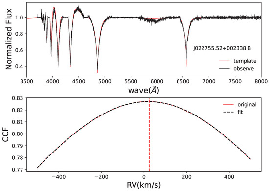
Figure 1.
(Top): The red solid line indicates the normalized template spectrum, and the black solid line is the normalized observed spectrum. (Bottom): The red solid line shows the original CCF curve, the black dashed line shows the fitted CCF curve, and the red dashed line shows the maximum value corresponding to the fitted CCF curve.
To obtain the error in the RV estimation, the Monte Carlo method was adopted. For each observed spectrum, many simulated spectra were generated based on the error of the flux at each pixel, and the CCF curves of these simulated spectra were calculated to obtain the RVs of each simulated spectrum. The standard deviation of the RVs of these simulated spectra was taken as the error of the RVs. For each observed spectrum, we generated 100 simulated flux values at each pixel by adding the error that followed the Gaussian distribution. This allowed us to generated 100 simulated spectra for each observed spectrum. Figure 2 and Figure 3 show the normalized spectra and corresponding CCF curves for the 100 simulated and 1 observed spectra, respectively. It is clear that the simulated spectra we generated are uniformly distributed around the observed spectra. The CCF curves of the observed spectra are higher than those of the simulated spectra due to the added error in the simulated spectra, which causes the SNR ratio to be inferior to that of the originally observed spectra.
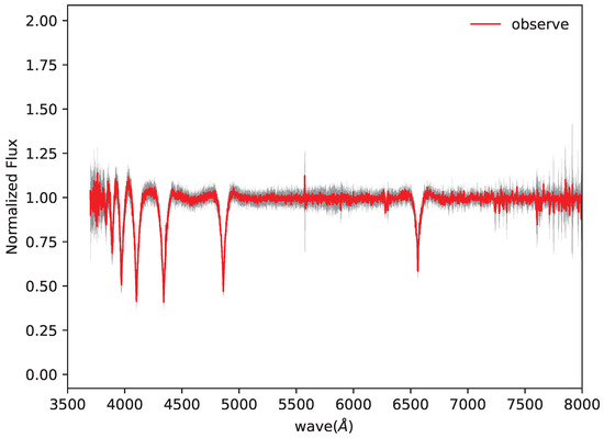
Figure 2.
The normalized spectra of the generated 100 simulated spectra (gray line) and the normalized spectra of the observed spectra (red line).

Figure 3.
CCF curves of 100 simulated spectra (black line) and CCF curves of observed spectra (red line).
Figure 4 shows the relation between the errors of RVs and the SNR. As the spectral SNR increases, the error of RVs becomes smaller. It should be noted that there are some WDs with zero RV error at a very small SNR. After our subsequent examination of the CCF images, we find that these are a sample of WDs with anomalous CCF images, and we discuss these WDs separately below.
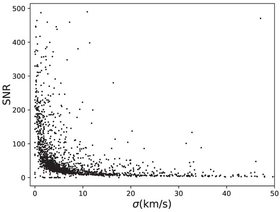
Figure 4.
The SNR of spectra vs. the RV uncertainties of the WDs.
2.3. DA White Dwarf Binary Candidates
To obtain WD binary candidates with high confidence, we first constrained the error of the RV to be within 30 km/s, which helped to select more accurate WD binary candidates. For a WD target with only two observations, if the RV difference was larger than twice the sum of errors of RV, we regarded it as a binary candidate. A target with more than two observations was considered a binary candidate if the difference between any two RVs was greater than the sum of the errors. The selection criteria were as follows:
- (1)
- < 30 km s;
- (2)
- For targets with only two observations:RV1, RV2 are the radial velocity from the two observation spectra.
For the targets with more than two observations, ( are the radial velocity values of any two spectra):
Finally, we obtained 60 DA WD binary candidates according to the above criteria. Table 1 shows the RVs of all DA WD binary candidates (top five objects; the full table can be found in the Supplementary Material).

Table 1.
Information on the top five objects.
3. Parameters of the DA WD Binary Candidates
3.1. and for WDs Binary Candidates and Single WDs
The BP-RP of the WD sample were obtained from the Gaia EDR3 [22], and we calculated the effective temperature () and surface gravity () of the WDs according to the method described in Ref. [23]. Figure 5 shows the distribution of and . The black solid line indicates the distribution of our selected DA WDs, and the red solid line indicates the distribution of WD binary candidates. There is no significant difference in the distribution of and between the WD binaries and the total sample of WDs. The peaks of and distribution located at 20,000 K and 8.0 dex for both binary candidates and the single WD sample.
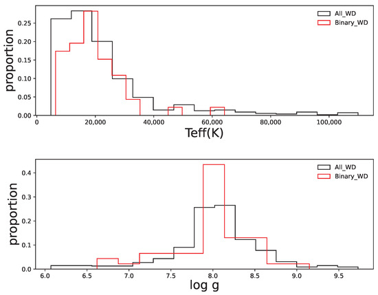
Figure 5.
Histograms of and ; the vertical coordinate indicates the percentage. Black: WD single stars. Red: WD binary candidates.
Ref. [4] certified the WD sample and calculated their parameter information based on the data published by SDSS DR14. Ref. [24] used Gaia astrometry and photometry fitted with synthetic pure H, pure He, and mixed H–He atmospheric models from the Gaia EDR3 data to estimate the parameter information for selected WDs. In order to verify the accuracy of our calculations and to identify the differences of the and from different survey data, we cross-matched the selected WD binary candidates with Refs. [4,24], respectively, and plotted the comparison of and of common stars given by different data, as shown in Figure 6.
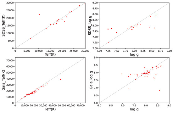
Figure 6.
Comparison of the , of white dwarfs provided by Gaia and SDSS with our calculated , of white dwarfs. The black solid lines are unit slope relationships. Top panel: Comparison of the and we calculated with the and calculated with the SDSS. Lower panel: Comparison of the and we calculated with and calculated with Gaia.
Matching our WD binary candidates with SDSS yields 19 WD spectra for common stars. Our agrees well with that by Ref. [4] using SDSS data. For , the agreement is good at around , and the value of calculated by [4] is larger compared to ours for and smaller compared to ours for .
For these homologous WDs, we found that four of them also have multiple observed spectra in the SDSS data, and we calculated their RVs based on these four multiple observed spectral data and found that all of them have RV variations. Table 2 shows the RVs of these WDs.
Table 2.
RVs of these homologous WDs.
Cross-matching with the Gaia data from Ref. [24] yielded 44 homologous stars. For the effective temperature, the two values agree well at temperatures less than 50,000 K. When the temperature is higher, the discrepancy is more obvious. For , it is more consistent overall but contains some targets with large deviations, which may be caused by observational constraints and the influence of the SNR.
3.2. Calculation and Comparison of Mass
After obtaining and , we can estimate the mass of the WDs according to the stellar evolution model. For DA WDs with effective temperatures above 3000 K, we use the cooling model of Ref. [25], and for effective temperatures below 3000 K, we use the cooling model of Ref. [2]. Figure 7 shows the histograms of the mass distribution of total sample and binary candidates. From the mass distribution, we find that the masses of WDs are mainly distributed around 0.6 M. The mass distribution of the DA WD binary candidates is not significantly different from that of the single WDs.
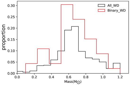
Figure 7.
Comparison of the mass distribution of WD binary candidates and single WDs. Black: WD single stars. Red: WD binary candidates.
Similarly, we compared the calculated masses of the WD binary candidates with those obtained from Refs. [4,24]. Figure 8 demonstrates the mass comparisons. Most of them are relatively consistent, and some of the member stars with large mass deviations are compatible with the deviations of and .
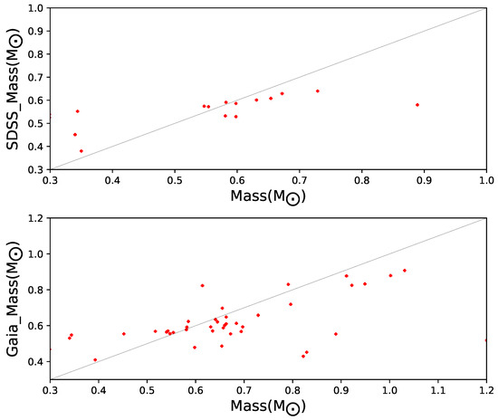
Figure 8.
The mass we calculated compared to the mass calculated by Refs. [4,24]. The black solid lines are unit slope relationships. The red dots indicate the corresponding sample stars’ parameters.
3.3. Gaia Hertzsprung–Russell Diagram
Hertzsprung–Russell (H-R) diagrams are often used to distinguish between different kinds of stars. To further investigate the relationship between DA WD binaries and normal WDs on the H–R diagram, we plotted the distribution of with mag in Figure 9. We calculated the mag and extinction using the dust map provided by Ref. [26]. The green triangles indicate the double WD binary candidates we selected, the blue hollow circles indicate WDMS (See Table 3), and the grey dots indicate the total DA WD sample. The position of WD distribution on the H–R diagram, as confirmed by spectroscopic methods, is an important piece of information used to filter WDs. Ref. [27] gave the boundary of the WD distribution on the H–R diagram based on this distribution position. In Figure 9, we indicate the boundary given by Ref. [27] with a black line. Based on the distribution characteristics of known WDMS systems in the H–R diagram [28,29,30], the WDMS system has absolute magnitudes fainter than the main sequence stars and is brighter than single WDs. The red dashed line in Figure 9 is the boundary where Ref. [28] chooses WDMS stars. The two stars in the gray box are found to belong to the main-sequence stars by our examination of the spectra due to their magnitude values close to the main-sequence stars.
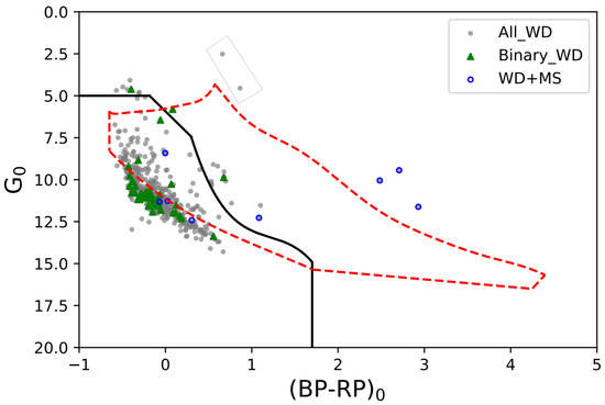
Figure 9.
The distribution of the WD binary candidates and the sample of general WDs on H–R diagram ( vs. absolute ). Green triangles: WD binary candidates; blue hollow circles: WD + MS stars obtained from spectroscopic examination; grey dots: total sample of DA WDs. The solid black line shows a color-cut and absolute magnitude selection scheme for searching for WDs using Gaia data proposed by Ref. [27]. The red dashed lines show the color–magnitude diagram selection scheme for searching for WDMS candidates based on Gaia EDR3 data by Ref. [28]. The two stars in the gray box are main-sequence stars that we found by examining their spectra.
Table 3.
DA + M binaries and four CVs.
It can be found on the H–R diagram that our WD binary candidates are mainly distributed in the range , . The fact that most binary candidates are not within the range of WDMS given by Ref. [28] indicates that our white dwarf binary candidates are mainly composed of two WDs.
4. ZTF Photometry and Examination of Abnormal Spectra
The photometric data provide us with a way to authenticate WD binaries. The Zwicky Transient Facility (ZTF) is a new generation of operational time-domain photometric telescopes located at Palomar Observatory. The g- and r-band surveys of the northern sky were carried out at 3760 square degrees per hour, with median limiting magnitudes of 20.8 and 20.6 mag in the g- and r-bands, respectively [31,32].
For the DA WD binary candidates, we used the photometric data of ZTF DR14 with the python package of lightkurve [33] for the period calculation and phase folding. Based on the ZTF data, we obtained two WD binary candidates with significant periods and calculated their light variation periods. Figure 10 shows light curves of the two objects (J182700.95 + 081030.3 RV error is 33 km/s). The information is given in Table 4.
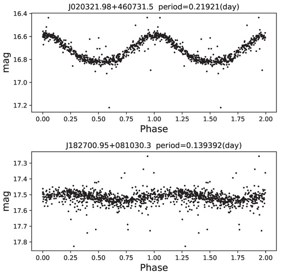
Figure 10.
Phase folding diagrams of J020321.98 + 460731.5 and J182700.95 + 081030.3.
Table 4.
Phase folding diagram of two of the white dwarf binary candidates with obvious light curve periods.
For the targets with anomalous CCF curves or with large errors in the calculated RVs, we examined their spectra by visual inspection. Twelve DA + M-type binaries and three cataclysmic binaries(CVs) were found. We analyzed the ZTF data of these DA + M-type binaries and three CV stars and obtained the period of one of the CVs. Figure 11 shows their power spectra and light curves. Figure 12 shows the spectrum of WD + MS (upper panel) and WD (lower panel). It is clear that the WD + MS binary spectra have two components. The left part shows the DA WD features, while the right part displays many molecular bands, the features of M-type stars. Table 3 lists the information of these objects.
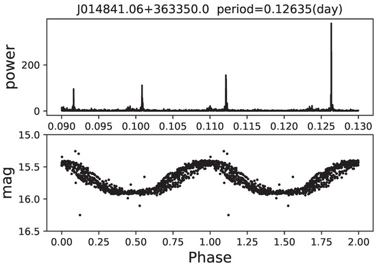
Figure 11.
Power spectrum light curve and phase folding diagram of J014841.06 + 363350.0.
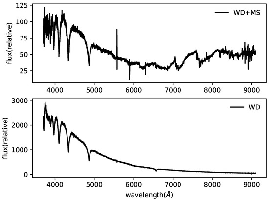
Figure 12.
Spectra of DA + MS binary and single WD. The upper panel shows the spectrum of WD + MS, while the lower panel shows the spectra of WD.
By cross-matching with the GCVS [34] catalog, we obtained three homologous star J023507.54 + 034356.8 (DA + M), J133941.12 + 484727.4 (CV), J084303.98 + 275149.6 (CV). By cross-matching with the VSX [35] variable star scale, we obtained homologous star J014841.06 + 363350.0 (CV), J172406.14 + 562003.0 (CV).
5. Conclusions
We obtained the spectra of 761 DA WDs with multiple observations from the LAMOST DR7 data of Ref. [15]. Their RVs were calculated according to the CCF method, and 60 WD binary candidates were selected through the RV variations combined with the CCF curves. Most binary candidates are located outside the WD + MS region in HRD. Thus, we surmise these binary candidates are composed of two WDs. The fraction of double WDs according to this study is about . Ref. [8] studied a subsample of the SPY dataset; they found that the double WD fraction among WDs is . The catalogue of WD + WD binary candidates in this paper is based on multiple observations of LAMOST spectra. Thus, the completeness cannot be guaranteed. Possible biases might come from the following factors:
- 1
- Only some of the WDs have multiple observations.
- 2
- The criteria of identifying binary candidates.
To investigate the physical properties of WD binary candidates and normal DA WDs, we calculated their mass, and . These physical parameters of DA WD binary candidates were analyzed and compared with the total sample of DA WDs. No clear distinctions between WD binaries and single WDs were found in terms of mass, , , and the CMD diagram. No distinction between Teff and log g for the full WD sample and the sample of binary candidates was the expected result, indicating that the locations in CMD are the same for the the full WD sample and binary candidates. We compared the calculated , , and masses with those calculated by Refs. [4,24], respectively, and there was found to be a good agreement.
With the ZTF photometric data, we obtained two targets with obvious light curve periods from the screened DA WD binary candidates and the light-change period of one CV. For the 58 WD binary candidates for which no period was found in ZTF, we could not estimate the upper and lower limits of the period with no ZTF data. To calculate the periods from radial velocities, at least 6 spectroscopic observations with a reasonable velocity phase distribution are needed. There are not enough data points of RV to estimate the periods. For the WDs with abnormal CCF curves, we found 11 DA + M-type binaries and 4 CVs by visual inspection. By matching with both GCVS and VSX variable star catalogs, we obtained a total of 5 homologous stars.
Supplementary Materials
The supporting information can be downloaded at: https://www.mdpi.com/article/10.3390/universe9040177/s1.
Author Contributions
Conceptualization, H.-H.Y. and J.-K.Z. methodology, J.-K.Z., W.-B.S. and H.-H.Y.; software, L.W. and J.-C.G.; formal analysis, H.-H.Y.; investigation, J.-K.Z.; resources, G.Z.; writing—original draft preparation, H.-H.Y.; writing—review and editing, H.-H.Y., J.-K.Z. and W.-B.S.; visualization, Z.-X.L.; supervision, G.Z., J.-K.Z. and W.-B.S.; project administration, G.Z.; funding acquisition, G.Z., J.-K.Z. and W.-B.S. All authors have read and agreed to the published version of the manuscript.
Funding
This paper was supported by the National Natural Science Foundation of China 11988101, 12273055, 11890694, 11973048, 11927804, U2031144, 12203006, the Innovation Project of Beijing Academy of Science and Technology (11000023T000002062763-23CB059) and National Key R&D Program of China under grant No. 2019YFA0405502. And also the support from the 2m Chinese Space Station Telescope project: CMS-CSST-2021-A10. And supports from National Natural Science Foundation of China No. 12073020, Scientific Research Fund of Hunan Provincial Education Department grant No. 20K124, Cultivation Project for LAMOST Scientific Payoff and Research Achievement of CAMS-CAS, the science research grants from the China Manned Space Project with No. CMS-CSST-2021-B05.
Data Availability Statement
The full data of Table 1 can be extracted at the following link: https://pan.baidu.com/s/1LyZ9aFXuuXYtZ-egXSRcDA?pwd=vuxi.
Acknowledgments
We thank National Natural Science Foundation of China 11988101, 12273055, 11890694, 11973048, 11927804, U2031144, 12203006, the Innovation Project of Beijing Academy of Science and Technology (11000023T000002062763-23CB059) and National Key R&D Program of China under grant No. 2019YFA0405502. We also acknowledge the support from the 2m Chinese Space Station Telescope project: CMS-CSST-2021-A10. And acknowledges supports from National Natural Science Foundation of China No. 12073020, Scientific Research Fund of Hunan Provincial Education Department grant No. 20K124, Cultivation Project for LAMOST Scientific Payoff and Research Achievement of CAMS-CAS, the science research grants from the China Manned Space Project with No. CMS-CSST-2021-B05. Guoshoujing Telescope (the Large Sky Area Multi-Object Fiber Spectroscopic Telescope LAMOST) is a National Major Scientific Project built by the Chinese Academy of Sciences. Funding for the project has been provided by the National Development and Reform Commission. LAMOST is operated and managed by the National Astronomical Observatories, Chinese Academy of Sciences.
Conflicts of Interest
The authors declare no conflict of interest.
References
- Doherty, C.L.; Gil-Pons, P.; Siess, L.; Lattanzio, J.C.; Lau, H.H.B. Super- and massive AGB stars—IV. Final fates–initial-to-final mass relation. Mon. Not. R. Astron. Soc. 2014, 446, 2599–2612. [Google Scholar] [CrossRef]
- Fontaine, G.; Brassard, P.; Bergeron, P. The Potential of White Dwarf Cosmochronology1. Publ. Astron. Soc. Pac. 2001, 113, 409. [Google Scholar] [CrossRef]
- Heger, A.; Fryer, C.L.; Woosley, S.E.; Langer, N.; Hartmann, D.H. How Massive Single Stars End Their Life. Astrophys. J. 2003, 591, 288. [Google Scholar] [CrossRef]
- Kepler, S.O.; Pelisoli, I.; Koester, D.; Reindl, N.; Geier, S.; Romero, A.D.; Ourique, G.; Oliveira, C.d.P.; Amaral, L.A. White dwarf and subdwarf stars in the Sloan Digital Sky Survey Data Release 14. Mon. Not. R. Astron. Soc. 2019, 486, 2169–2183. [Google Scholar] [CrossRef]
- Shipman, H.L. Masses and radii of white-dwarf stars. III. Results for 110 hydrogen-rich and 28 helium-rich stars. Astrophys. J. 1979, 228, 240–256. [Google Scholar] [CrossRef]
- McCook, G.P.; Sion, E.M. A Catalog of Spectroscopically Identified White Dwarfs. Astrophys. J. Suppl. Ser. 1999, 121, 1. [Google Scholar] [CrossRef]
- Duquennoy, A.; Mayor, M. How Many Single Stars Among Solar Type Stars? In Bioastronomy: The Search for Extraterrestial Life — The Exploration Broadens; Heidmann, J., Klein, M.J., Eds.; Springer: Cham, Switzerland, 1991; Volume 390, pp. 39–43. [Google Scholar] [CrossRef]
- Maoz, D.; Hallakoun, N. The binary fraction, separation distribution, and merger rate of white dwarfs from SPY. Mon. Not. R. Astron. Soc. 2017, 467, 1414–1425. [Google Scholar] [CrossRef]
- Ren, J.J.; Rebassa-Mansergas, A.; Parsons, S.G.; Liu, X.W.; Luo, A.L.; Kong, X.; Zhang, H.T. White dwarf-main sequence binaries from LAMOST: The DR5 catalogue. Mon. Not. R. Astron. Soc. 2018, 477, 4641–4654. [Google Scholar] [CrossRef]
- Nayak, P.K.; Ganguly, A.; Chatterjee, S. Hunting Down White Dwarf–Main Sequence Binaries Using Multi-Wavelength Observations. arXiv 2022, arXiv:2212.09800. [Google Scholar]
- Shen, K.J.; Boubert, D.; Gänsicke, B.T.; Jha, S.W.; Andrews, J.E.; Chomiuk, L.; Foley, R.J.; Fraser, M.; Gromadzki, M.; Guillochon, J.; et al. Three Hypervelocity White Dwarfs in Gaia DR2: Evidence for Dynamically Driven Double-degenerate Double-detonation Type Ia Supernovae. Astrophys. J. 2018, 865, 15. [Google Scholar] [CrossRef]
- Maselli, A.; Marassi, S.; Branchesi, M. Binary white dwarfs and decihertz gravitational wave observations: From the Hubble constant to supernova astrophysics. Astron. Astrophys. 2020, 635, A120. [Google Scholar] [CrossRef]
- Ablimit, I. The magnetized white dwarf + helium star binary evolution with accretion-induced collapse. Mon. Not. R. Astron. Soc. 2022, 509, 6061–6067. [Google Scholar] [CrossRef]
- Chandra, V.; Hwang, H.C.; Zakamska, N.L.; Gänsicke, B.T.; Hermes, J.J.; Schwope, A.; Badenes, C.; Tovmassian, G.; Bauer, E.B.; Maoz, D.; et al. A 99 minute Double-lined White Dwarf Binary from SDSS-V. Astrophys. J. 2021, 921, 160. [Google Scholar] [CrossRef]
- Kong, X.; Luo, A.L. Identification of White Dwarfs from Gaia EDR3 via Spectra from LAMOST DR7. Res. Notes Am. Astron. Soc. 2021, 5, 249. [Google Scholar] [CrossRef]
- Tan, L.; Mei, Y.; Liu, Z.; Luo, Y.; Deng, H.; Wang, F.; Deng, L.; Liu, C. Hot subdwarf candidates from LAMOST DR7. Astrophys. J. Suppl. Ser. 2022, 259, 5. [Google Scholar] [CrossRef]
- Tonry, J.; Davis, M. A survey of galaxy redshifts. I. Data reduction techniques. Astron. J. 1979, 84, 1511–1525. [Google Scholar] [CrossRef]
- Zhang, B.; Liu, C.; Deng, L.C. Deriving the Stellar Labels of LAMOST Spectra with the Stellar LAbel Machine (SLAM). Astrophys. J. Suppl. Ser. 2020, 246, 9. [Google Scholar] [CrossRef]
- Zhang, B.; Li, J.; Yang, F.; Xiong, J.P.; Fu, J.N.; Liu, C.; Tian, H.; Li, Y.B.; Wang, J.X.; Liang, C.X.; et al. Self-consistent Stellar Radial Velocities from LAMOST Medium-resolution Survey DR7. Astrophys. J. Suppl. Ser. 2021, 256, 14. [Google Scholar] [CrossRef]
- Koester, D. White dwarf spectra and atmosphere models. Mem. Della Soc. Astron. Ital. 2010, 81, 921–931. [Google Scholar]
- Chandra, V.; Hwang, H.C.; Zakamska, N.L.; Budavári, T. Computational tools for the spectroscopic analysis of white dwarfs. Mon. Not. R. Astron. Soc. 2020, 497, 2688–2698. [Google Scholar] [CrossRef]
- Collaboration, G.; Brown, A.G.A.; Vallenari, A.; Prusti, T.; de Bruijne, J.H.J.; Babusiaux, C.; Biermann, M.; Creevey, O.L.; Evans, D.W.; Eyer, L.; et al. Gaia Early Data Release 3. Summary of the contents and survey properties. Astron. Astrophys. 2021, 649, A1. [Google Scholar] [CrossRef]
- Guo, J.; Zhao, J.; Zhang, H.; Zhang, J.; Bai, Y.; Walters, N.; Yang, Y.; Liu, J. White dwarfs identified in LAMOST Data Release 5. Mon. Not. R. Astron. Soc. 2022, 509, 2674–2688. [Google Scholar] [CrossRef]
- Gentile Fusillo, N.P.; Tremblay, P.E.; Cukanovaite, E.; Vorontseva, A.; Lallement, R.; Hollands, M.; Gänsicke, B.T.; Burdge, K.B.; McCleery, J.; Jordan, S. A catalogue of white dwarfs in Gaia EDR3. Mon. Not. R. Astron. Soc. 2021, 508, 3877–3896. [Google Scholar] [CrossRef]
- Wood, M.A. Theoretical White Dwarf Luminosity Functions: DA Models. In White Dwarfs; Koester, D., Werner, K., Eds.; Springer: Cham, Switzerland, 1995; Volume 443, p. 41. [Google Scholar] [CrossRef]
- Green, G.M.; Schlafly, E.; Zucker, C.; Speagle, J.S.; Finkbeiner, D. A 3D Dust Map Based on Gaia, Pan-STARRS 1, and 2MASS. Astrophys. J. 2019, 887, 93. [Google Scholar] [CrossRef]
- Gentile Fusillo, N.P.; Tremblay, P.E.; Gänsicke, B.T.; Manser, C.J.; Cunningham, T.; Cukanovaite, E.; Hollands, M.; Marsh, T.; Raddi, R.; Jordan, S.; et al. A Gaia Data Release 2 catalogue of white dwarfs and a comparison with SDSS. Mon. Not. R. Astron. Soc. 2019, 482, 4570–4591. [Google Scholar] [CrossRef]
- Rebassa-Mansergas, A.; Solano, E.; Jiménez-Esteban, F.M.; Torres, S.; Rodrigo, C.; Ferrer-Burjachs, A.; Calcaferro, L.M.; Althaus, L.G.; Córsico, A.H. White dwarf-main-sequence binaries from Gaia EDR3: The unresolved 100 pc volume-limited sample. Mon. Not. R. Astron. Soc. 2021, 506, 5201–5211. [Google Scholar] [CrossRef]
- Inight, K.; Gänsicke, B.T.; Breedt, E.; Marsh, T.R.; Pala, A.F.; Raddi, R. Towards a volumetric census of close white dwarf binaries—I. Reference samples. Mon. Not. R. Astron. Soc. 2021, 504, 2420–2442. [Google Scholar] [CrossRef]
- Pelisoli, I.; Vos, J. Gaia Data Release 2 catalogue of extremely low-mass white dwarf candidates. Mon. Not. R. Astron. Soc. 2019, 488, 2892–2903. [Google Scholar] [CrossRef]
- Masci, F.J.; Laher, R.R.; Rusholme, B.; Shupe, D.L.; Groom, S.; Surace, J.; Jackson, E.; Monkewitz, S.; Beck, R.; Flynn, D.; et al. The Zwicky Transient Facility: Data Processing, Products, and Archive. Publ. Astron. Soc. Pac. 2019, 131, 018003. [Google Scholar] [CrossRef]
- Bellm, E.C.; Kulkarni, S.R.; Barlow, T.; Feindt, U.; Graham, M.J.; Goobar, A.; Kupfer, T.; Ngeow, C.C.; Nugent, P.; Ofek, E.; et al. The Zwicky Transient Facility: Surveys and Scheduler. Publ. Astron. Soc. Pac. 2019, 131, 068003. [Google Scholar] [CrossRef]
- Collaboration, L.; Cardoso, J.V.d.M.; Hedges, C.; Gully-Santiago, M.; Saunders, N.; Cody, A.M.; Barclay, T.; Hall, O.; Sagear, S.; Turtelboom, E.; et al. Lightkurve: Kepler and TESS Time Series Analysis in Python. Astrophysics Source Code Library. 2018. Available online: http://xxx.lanl.gov/abs/1812.013 (accessed on 6 January 2023).
- Samus’, N.N.; Kazarovets, E.V.; Durlevich, O.V.; Kireeva, N.N.; Pastukhova, E.N. General catalogue of variable stars: Version GCVS 5.1. Astron. Rep. 2017, 61, 80–88. [Google Scholar] [CrossRef]
- Watson, C.L.; Henden, A.A.; Price, A. The International Variable Star Index (VSX). Soc. Astron. Sci. Annu. Symp. 2006, 25, 47. [Google Scholar]


Disclaimer/Publisher’s Note: The statements, opinions and data contained in all publications are solely those of the individual author(s) and contributor(s) and not of MDPI and/or the editor(s). MDPI and/or the editor(s) disclaim responsibility for any injury to people or property resulting from any ideas, methods, instructions or products referred to in the content. |
© 2023 by the authors. Licensee MDPI, Basel, Switzerland. This article is an open access article distributed under the terms and conditions of the Creative Commons Attribution (CC BY) license (https://creativecommons.org/licenses/by/4.0/).