Abstract
This article presents a classical potential used to describe nucleon–nucleon interactions at intermediate energies. The potential depends on the relative momentum of the colliding nucleons and can be used to describe interactions at low momentum transfer mimicking the Pauli exclusion principle. We use the potential with molecular dynamics to study finite nuclei, their binding energy, radii, symmetry energy, and a case study of collisions.
1. Introduction
In recent years, the field of nuclear physics has witnessed an explosion in interest on a large variety of nuclear phenomena, ranging from the structure of nuclei and their decay modes, passing through the study of exotic nuclei, and up to the properties of neutron stars. In particular, the study of heavy-ion collisions at intermediate energies requires the use of theoretical models, which are the main tool to extract information from such reactions.
Most models intend to reproduce reactions. Until now, it has been a trade-off; while most researchers study nuclear reactions using models in which the nucleons (or their avatars) interact via an average mean field, a few others use classical dynamics with direct nucleon–nucleon interactions. Those using mean field methods sacrifice clusterization, fragment formation, and many other critical phenomena for the inclusion of some quantum and semi-quantum features. On the other hand, those using classical dynamics fail in including quantum features but gain in preserving nucleon–nucleon correlations, statistical fluctuations, phase changes, and all critical phenomena of the upmost importance in the later stages of fragmentation reactions.
In an odd complementarity, the quantum aspects of mean field models aid in achieving a proper energy distribution through the early stages of the reaction, while failing at fragmenting the system in the latter stage of the collision, whereas the classical methods excel in the latter phase but cannot guarantee proper reaction dynamics in the early part of the reaction.
By themselves, different mean field models from the two basic families, Boltzmann–Uhling–Uhlenbeck (BUU) and Quantum Molecular Dynamics (QMD), show discrepancies in their predictions. The results of a recent comparison of different models indicate that they vary in the stability of the initialized nuclei, the effectiveness of Pauli blocking in nucleon–nucleon collisions, as well as other predicted flow observables, mostly due to differences in the initialization of the systems, the treatment of the collision integral, and other much-entangled effects [1].
The latter are probably due to the operator’s selections of number of “test particles” (i.e., the avatars) and, more importantly, to the artificial fluctuations included by hand both in QMD and in the Langevin framework of BUU. Although fragmentation was not studied in such comparison, it continues to be the Achilles’ heel of all such models [2,3,4,5,6]; to compare to final yields, final matter density distributions must be used as input to “afterburner” codes, such as the Statistical Multifragmentation Model [7], and the like; for a description of the Antisymmetrized Molecular Dynamics (AMD) model with an added mechanism for fragment formation, see [8], and, for a recent application of AMD and SMS, see [9].
On the other hand, in spite of violating quantum principles, classical dynamics models (such as classical molecular dynamics) are capable of reproducing both the out-of-equilibrium and the equilibrium parts of a collision. Indeed, classical molecular dynamics (CMD) models are able to describe non-equilibrium dynamics, hydrodynamic flow, and changes of phase without adjustable parameters, neck fragmentation [10], phase transitions [11], critical phenomena [12,13], caloric curve [14,15], and isoscaling [16] in nuclear reactions, as well as in the formation of nuclear pasta in infinite systems [17,18,19].
[A particular success of CMD over mean field models is the calculation of symmetry energy at clustering densities and temperatures [20], which showed good agreement with experimental data [21,22,23]. This corroborated the Natowitz conjecture that the asymptotic limit of would not tend to zero at small densities as predicted by mean-field theories.]
In spite of such successes, CMD lacks all quantum effects which can affect the reaction dynamics in, at least, two fronts: its energy distribution and wave mechanics. Nucleons in bound nuclei have discrete energy levels, as ruled by Fermi–Dirac statistics, with their occupation regulated by the Pauli exclusion principle. A second effect is the lack of wave features of the particles, which becomes dominant whenever the mean interparticle distance is smaller than the mean thermal de Broglie wavelength. Although the limits of such deficiencies have been estimated [24], and tend to disappear at sub-saturation density and sub-critical temperatures, their effects in the various stages of the collision, especially those that happen at saturation and higher densities and cold temperatures, are not known. A formulation to correct for these inadequacies is the topic of this work.
In this work, we first introduce, in Section 2, a classical two-boy potential that mimics the effect of the Pauli exclusion principle by de-enhancing interactions between nucleons that are too close in phase space. We then use such potential, in Section 3, to construct “nuclei” with binding energies and radii close to the experimental values, and, in Section 4, the symmetry energy of such nuclei is studied. Next, in Section 5, we test the usefulness of the constructed nuclei to simulate nuclear reactions. We finally present a series of observations in Section 6, along with an outlook for future uses of the potentials developed.
2. Nuclear Potentials and the Quantum Problem
Classical dynamical methods use point particles to represent nucleons interacting through pair potentials. This approach started decades ago and has advanced ever since [17,25,26,27,28,29,30,31,32]. Classical dynamics has evolved from using a common mean field plus a residual scattering in an adaptation of Nordheim’s propagation of individual nucleons [33], to a full fledge incorporation of nucleon–nucleon potentials [26,27,32,34] created ad hoc to mimic nuclear properties, such as binding energy, saturation density, and nucleon–nucleon scattering cross section, among others. Some of the potentials used to study nuclear reactions can be found in [24,25,27,28,34,35,36,37,38,39,40], while those that have been used to study infinite nuclear systems (as expected to exist in neutron stars) are [17,29,30,31,35,36,37,38].
Reiterating, in bound clusters, such as cold nuclei, individual nucleons attain discrete energies distributed according to Fermi–Dirac statistics, with the occupation of such levels regulated by the Pauli exclusion principle. Although at high excitation energies the number of levels available for the nucleons increases exponentially and render Pauli blocking practically obsolete [24], at lower temperatures, the occupation of levels increases and the nucleon dynamics faces prohibiting energy and momentum transfers in nucleon–nucleon collisions. Since in heavy-ion collisions at intermediate energies the initially cold nuclei will compress to supra-saturation densities, Pauli blocking is expected to play a role in suppressing some of the nucleon–nucleon interactions. As the compressed system heats up to a few MeVs, and the energy level density becomes more dense, the system will approach a classical level. Later, when the system cools and expands, Pauli exclusion will again regulate final-stage interactions, including fragmentation.
This suggests that, for a classical potential to mimic the Pauli blocking, it should try to reduce the number of collisions occurring in cold nuclear systems, i.e., at low momentum transfer, or in near proximity in phase space.
2.1. Adding Pauli Blocking to a Potential
One way to simulate Pauli blocking in classical collisions is to introduce a momentum-dependent repulsion that would de-enhance nucleon–nucleon collisions at low energies and low momentum transfer. This approach was first taken by Wilets et al. [26], followed up by Dorso and Randrup [41], and, in other approximation, by Boal et al. [42,43]. Subsequent efforts of Dorso and Randrup [28] managed to simulate the Pauli exclusion principle, provided nucleons with a realistic ground-state Fermi motion, but failed at endowing the model with an appropriate repulsion between equal nucleons.
Recently, in a study preliminary to this one [44], we followed the footsteps of Dorso and Randrup, and introduced a momentum-dependent repulsive potential that gradually reduces the strength of the nuclear potential as a function of the relative momentum of the interacting nucleons. The nuclear part of the potential was crafted with Lennard–Jones-like two-body interactions plus a standard Coulomb repulsion between protons. The parameters of the potential were adjusted, once and for all, to yield infinite systems with the proper saturation energy and compressibility over a broad range of temperatures and densities. The resulting potential managed to solve the problem of [28], namely, avoiding the formation of di-neutron structures, but, in spite of such improvements, when compared to experimental values, the resulting radii of bound nuclei of [44] were underpredicted by a large 15%, and the binding energies were overbound by a huge 50%.
Concluding, the motivation for this study is to develop a model that would maintain the advantages of classical models, respect the Pauli exclusion principle, and prevent the formation of nonphysical states, while yielding stable nuclei with the correct binding energy and radii. In this work, we present a potential that solves these problems, and use it to calculate the radii, binding energy, symmetry energy, and demonstrate its usefulness in studying reactions, their evolution, and the calculation of final multiplicities.
2.2. The Potential
The proposed potential consists of a nuclear part, a “Pauli” part, and a Coulomb part. The Pauli potential is inspired on the work of Dorso and Randrup [41], and the nuclear part on [28]. The Pauli depends on the relative momenta of the interacting nuclei. Defining a dimensionless distance in phase space between any pair of nucleons i and j as , where , and , and the parameters and determine the volume in phase space that is excluded around each particle; the values of and are adjusted as to satisfy the uncertainty relation, . The Pauli part of the potential is:
with the scale factors MeV, MeV/c, and fm.
The strength of the was selected to attain the proper Fermi gas values. Notice that, different from our previous work [44], this potential does not have a cut-off distance to avoid discontinuities of long-range interactions occurring in collisions. It is worth mentioning that, although the value fm may give the impression that is nearly a constant within the nucleus and does not have much of an effect, this is not the case. As it will be seen in Section 3, the nucleus diameter (c.f. Figure 1) is substantially larger than , and, furthermore, in collisions, the scale for nucleon–nucleon interactions is set by the entire volume of the collision. In addition, it is important that , very close to the uncertainty relation, and slightly smaller than as expected from geometric considerations [41]. Other authors have used other values of (see, e.g., [45]), but this give-and-take game yields values of that lie outside the range of interest for building static nuclei and for simulating collisions; we, thus, did not find strong reasons for varying the parameters used in the originals works [28,41].
In summary, the potential adds a modulating term that introduces a repulsive force between equal nucleons at short values of and , thus forbidding their interaction. Indeed, at and , the potential (1) becomes , generating a kinetic energy resembling the“Fermi energy” expected under those circumstances. The blue line of Figure 2 shows the Pauli potential for the case of zero momentum transfer, .
The nuclear part of the potential is:
where the parameters MeV and MeV were determined by fitting the binding energies and radii of atomic nuclei. The other parameters, , m, and n, were determined from the experimental value of the nuclear binding energy of the nucleus (as explained in [44]) to be fm, , and , which correspond to a binding energy at saturation density of MeV. The fitting of the parameters , , and was obtained by a random walk in the parameter space, starting from the values of [46], while nuclei of various sizes were crafted (with the procedure explained in Section 3), and their binding energy and radii were calculated, until a good agreement with experimental data of [47] was obtained.

Figure 1.
Radii of simulated nuclei compared to experimental data. The data points in blue correspond to commonly accepted experimental values [47].
Figure 1.
Radii of simulated nuclei compared to experimental data. The data points in blue correspond to commonly accepted experimental values [47].


Figure 2.
Nuclear, Pauli, and Coulomb potentials. The blue line corresponds to the spatial factor of the Pauli potential, , plotted as a function of r.
Figure 2.
Nuclear, Pauli, and Coulomb potentials. The blue line corresponds to the spatial factor of the Pauli potential, , plotted as a function of r.

It is worth mentioning that the neutron–neutron term of the potential (2) was introduced to prevent the formation of di-neutrons, while the proton–proton one was incorporated only to preserve isotopic symmetry, as the formation of di-protons is impeded by .
Finally, for the Coulomb potential, we use the point-charge repulsion:
where e is the elementary electric charge, and thus MeV fm. These potentials are shown in Figure 2.
3. Nuclei
The previous potential was used to create clusters of nucleons to simulate nuclei. This was achieved by confining nucleons inside a three-dimensional quadratic external potential, and allowing them to evolve by molecular dynamics. Initially, the nucleons were endowed with momenta corresponding to a temperature MeV according to a Maxwell distribution, and were cooled down gradually by reducing their momenta until reaching a temperature of MeV, at which point the external potential was removed. For the fitting of the nuclear parameters, the heating-cooling procedure was repeated once to make sure that the nuclei were self-stable, and to obtain robust averages of the binding energy and radii.
Different from our previous study [44], here we use classical molecular dynamics with potentials (1)–(3), instead of the Metropolis–Monte Carlo (MMC) method [48]; the MMC method, however, was used only at the end to verify that both methods yielded the same final binding energy of the cold nuclei. It must be observed that the Pauli potential (1) is not separable, and the usual symplectic integrators of the equations of motion used in molecular dynamics cannot guarantee the conservation of energy. Fortunately, for the present case of molecular dynamics with thermostats, the energy is obviously not conserved. For the calculation of reactions, as presented in Section 5, the integration occurs over short times, which has been shown to limit the divergence of conserved quantities [49].
The radii of several nuclear-like clusters bound with the potentials (1)–(3) are presented in Figure 1 and compared to experimental values. The radii were calculated as the r.m.s value of the position of the nucleons in the “ground state” ( MeV) of the nuclei constructed with the procedure presented before. The figure also includes the curve that corresponds to the best fit of the radii of the simulated nuclei.
Table 1 and Figure 3 show the binding energy per nucleon corresponding to the nuclei of Figure 1. The results of the simulation show a much better agreement with the experimental data of [47], and a large improvement with respect to the previous model [44]. For comparison with other classical models, see the Simple Semi-classical Potential of Horowitz and coworkers [30], and that of Dorso and Alcain [50].

Table 1.
Binding energy per nucleon and radius of selected nuclei.
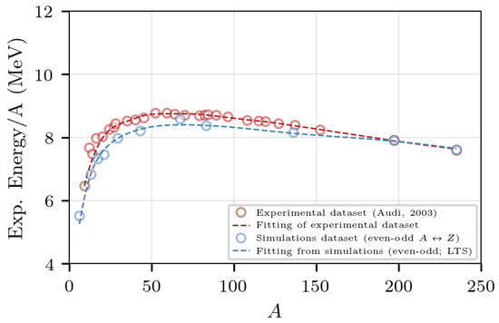
Figure 3.
Binding energy obtained for the nuclei of Figure 1. The blue dashed line is the fit to the energies of the simulated nuclei using the least-trimmed-square estimator (LTS) [47].
The figure also shows a semi empirical mass formula fit of the values of the form
with the coefficients shown in Table 2; the values were obtained by fitting the semi empirical mass formula to the binding energies of the simulated nuclei using the least-trimmed-square estimator (LTS). The resulting fit corresponds to the blue dashed line of Figure 3. The values of Audi [47], Rholf [51], Dorso [39], and of the Generalized liquid drop model [52] are presented for comparison.
Table 2.
Coefficients of the semi empirical mass formula.
It must be mentioned that the Coulomb and symmetry terms of Equation (4) depend explicitly on A and Z, which introduces discontinuities for different isotopes of the same element, and such fluctuations are more noticeable around . Because of this double A–Z dependence, the fit required a particular procedure which is summarized in Appendix A.
4. Symmetry Energy
The variation of the binding energy as a function of the isotopic number became relevant when radioactive beam facilities became able to produce nuclei away from the stability valley. Such variation, known as the nuclear symmetry energy, is needed to study topics ranging from nuclear structure to astrophysical processes [53].
Historically, Weizsäcker introduced an asymmetry term to his 1935 parametrization of the nuclear binding energy to enhance binding of nuclei with an equal number of protons and neutrons [54]. When the mass formula was generalized to be density-dependent, such term was modified to include the role of isospin in the density-dependent asymmetry term, [55]. The symmetry energy is defined as:
with and with .
In this case, the symmetry energy can be evaluated from the binding energies of the isotopic nuclei data constructed by the method presented before. For this purpose, several instances of a specific nucleus are constructed, and the average binding energy is obtained through , where N is the number of nuclei constructed. Figure 4 illustrates the convergence of as N increases, for three different isotopes of . In what follows, N is set to 20.
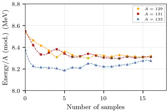
Figure 4.
Convergence of the magnitude of the average binding energy of various isotopes of as a function of the number of samples.
Figure 5 shows the average values of the binding energies of the isotopes , , and , as a function of the proton asymmetry x; the values were obtained as averages of 20 constructions of the isotopes. For comparison, we also present the experimental values for isotopes of taken from [56]. In addition, a quadratic fit obtained by least squares is shown, , from which the symmetry energy can be obtained to be MeV. This value is not too distant from the symmetry energy of 70 MeV obtained in a previous molecular dynamics study of nuclear matter at MeV and density [18], but it is outside the generally accepted values of 30–50 MeV obtained with microscopic field theories for isospin symmetric matter at saturation density [53,57]. In passing, we use the same method to fit the experimental data and extract the corresponding symmetry energy, the resulting fit is , and its symmetry energy is 90.48/4 = 22.62 MeV, somewhat below the accepted range from microscopic field theories.
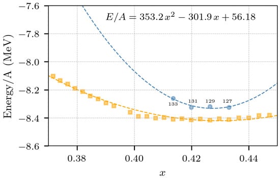
Figure 5.
Average values of the binding energy of various isotopes of obtained from simulations (blue) and least-squares fit. In addition, the experimental values of the binding energies of isotopes (orange) and a corresponding quadratic fit are shown.
5. Collisions
The ultimate goal of any model is to reproduce experimental observables, which, in the case of nuclear physics, are obtained through reactions. In this last section, we present a first attempt to reproduce nuclear collisions with “nuclei” created as described in Section 3 with the potentials shown in Section 2.
As a test case, we examine the reaction of in collisions with impact parameters ranging from fm to fm, at a center-of-mass energy of 33 AMeV. For this proof of concept, 30 collisions were performed, each with random rotations of the colliding nuclei; Figure 6 shows a sequence of snapshots of one of such collisions. The nuclei were prepared cold as explained in Section 3, and the initial separation of the colliding nuclei was 40 fm. The evolution of the collision was simulated using molecular dynamics integrated with the Leapfrog/Midpoint Euler method. The evolution time was 300 MeV/c, and the position and momenta of each nucleon was registered at intervals of 10 MeV/c. The identification of fragments was carried out by means of a minimum spanning tree algorithm, using a cut-off distance of 10 fm, eliminating loops between nucleons.
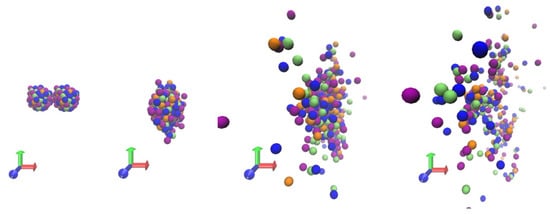
Figure 6.
Four snapshots of the reaction at 33 AMeV and zero impact parameter.
The evolution of the reaction can be analyzed by tracking the average size of the fragments being produced in the reaction. Figure 7 shows the average (over 30 collisions) of the size of all fragments being produced, , as a function of time. Clearly, at early times, say MeV/c, the two nuclei merge to produce a single fragment of with negligible dispersion . As evaporation and fragmentation set in, intermediate-mass fragments are produced and continue to evaporate.
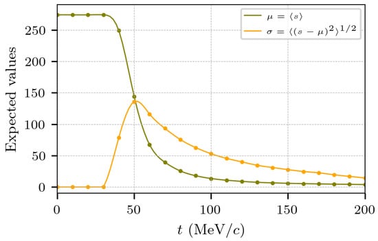
Figure 7.
Evolution of the average size of fragments being produced, , as a function of time, in 30 reactions of at 33 AMeV and . In addition, the dispersion is shown.
The fragment multiplicity existing at different times during the collision is shown in Figure 8. The top panel corresponds to early times when the colliding nuclei merge together, the middle one is the mass distribution when the dispersion reaches its maximum, and the bottom one is more similar to the asymptotic case without any large fragment left.
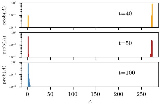
Figure 8.
Fragment multiplicity at different times during the collision, obtained from 30 reactions of at 33 AMeV and .
Likewise, if we look at all the fragments produced during the entire evolution of the collisions, we find what is presented in Figure 9. The entire multiplicity obtained in the 30 collisions of at 33 AMeV, and shows a clearly noticeable log-log relationship with the mass fragments. The particles produced with until are produced by evaporation, and the fragments larger than were produced early in the reaction.
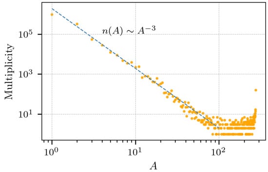
Figure 9.
Added multiplicity of 30 collisions of at 33 AMeV and . Clearly noticeable is a power law relationship of the form between the multiplicity n and the mass fragments s.
Repeating the collisions for impact parameters 1, 2, and 3 fm, and for 50 collisions, we obtain similar multiplicities, as seen in Figure 10. The power law, however, is lost for intermediate mass fragments of . Indeed, the power law wanes as the impact parameter increases away from head-on collisions. This is due to the fact that, as b increases, more nucleons become simple observers and do not participate in the sharing of momenta and energy; this effect produces an extreme “bump” for fm at around A 30.
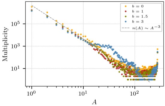
Figure 10.
Added multiplicity of 30 collisions of at 33 AMeV and various impact parameters. The power law relationship is lost for fragments of .
At a difference from the potential proposed in [28], our Pauli potential, Equation (1), contains only repulsive forces between equal nucleons, and thus de-enhances the formation of unphysical species such as di-neutrons, tri-neutrons, etc. To verify this, we examined the particle production formed during the evolution of 50 collisions of at 33 AMeV and at fm. Figure 11 shows the relative abundance of di-neutrons, tri-neutrons, etc. compared to the free neutrons. It is easy to see that the number of di-neutrons that appear during the collisions is two orders of magnitude less than the production of neutrons, and that higher multi-neutron compounds have even smaller probabilities of being produced; these exotic objects are energetically unstable and exist only for short times during the reaction.
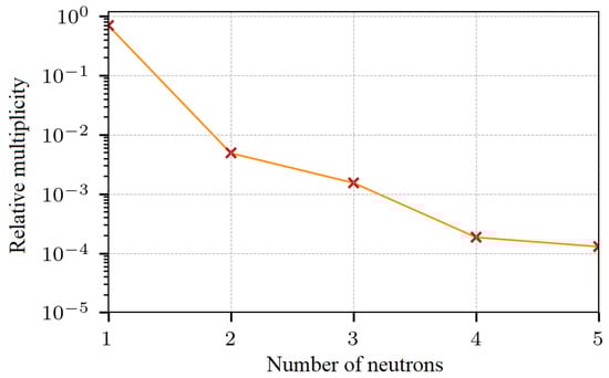
Figure 11.
Relative production of pure neutron compounds formed during the evolution of 50 collisions of at 33 AMeV and at fm, normalized to the number of free neutrons.
6. Conclusions
In this work, we introduced a classical nucleon–nucleon potential that depends on the relative momenta of the colliding nucleons. The potential has the ability to mimic the Pauli exclusion principle by reducing interactions at low momentum transfer, preserving volume in phase space.
The potential was used to construct “nuclei” using a method of successive cooling and heating until reaching appropriate low energies. The parameters of the potential were adjusted to attain appropriate values of their binding energies and radii and, as displayed in Figure 1, Figure 3, Figure 5, and Table 1, the resulting values are quite acceptable. Similarly, the symmetry energy of the self-bound nuclei was calculated, yielding values in the range comparable to other estimations.
Besides the static properties, the nuclei were also used to study collisions. Resorting to CMD calculations with a Midpoint Euler method, a quasi simplectic evolution was simulated. Several relevant observables were studied, namely, the fragment mass distributions during the evolution, the time-evolution of the average size of fragments, and the fragment multiplicity at asymptotic times. Finally, in these preliminary results, we have found that production of neutron clusters is irrelevant.
In future studies, we will focus on collisions and direct comparison to experimental data.
Author Contributions
Conceptualization, C.O.D.; methodology, C.O.D.; software, C.O.D. and G.F; validation, C.O.D., G.F. and J.A.L.; formal analysis, C.O.D., G.F. and J.A.L.; investigation, C.O.D., G.F. and J.A.L.; resources, C.O.D. and G.F.; data curation, G.F.; writing—original draft preparation, J.A.L.; writing—review and editing, C.O.D., G.F. and J.A.L.; visualization, G.F.; supervision, C.O.D.; project administration, C.O.D.; funding acquisition, C.O.D. All authors have read and agreed to the published version of the manuscript.
Funding
C.O.D. received support from the Carrera de Investigador CONICET, by CONICET grants PIP0871, PIP 2015-2017 GI, founding D4247(12-22-2016), and Inter-American Development Bank (IDB), Grant No. PICT 1692.
Data Availability Statement
The data presented in this study (i.e., data from simulations) are available on request from the corresponding author.
Conflicts of Interest
The authors declare no conflict of interest.
Appendix A
Equation (4) in Section 3 involves an explicit dependence on two variables, namely, A and Z, which introduces discontinuities for different isotopes of the same element; such fluctuations can be seen more noticeable around in Figure 3. Because of this double A–Z dependence, to determine a fit to the simulated data, the following procedure was used:
- The chosen model was , where , , and . This is a linear model with the parameters , , , and to be estimated. We intentionally avoided nonlinear models since these may lead to sub-optimal estimates. Notice, however, that the estimation is conditioned to the chosen isotopes ( values);
- The estimation was carried out by means of a least-trimmed-square estimator, which corresponds to the class of robust estimators, and is known to be more insensitive to outliers;
- The fitting shown in Figure 3 corresponds to the evaluation of the model at the data set. The values in between correspond to splines of order 2.
The resulting values of , , , and are listed in Table 2.
References
- Colonna, M.; Zhang, Y.X.; Wang, Y.J.; Cozma, D.; Danielewicz, P.; Ko, C.M.; Zhang, F.S. Comparison of Heavy-Ion Transport Simulations: Mean-field Dynamics in a Box. Phys. Rev. C 2021, 104, 024603. [Google Scholar] [CrossRef]
- Bertsch, G.F.; Gupta, S.D. A guide to microscopic models for intermediate energy heavy ion collisions. Phys. Rep. 1988, 160, 190. [Google Scholar] [CrossRef]
- Danielewicz, P. Determination of the mean-field momentum-dependence using elliptic flow. Nucl. Phys. A 2000, 673, 375. [Google Scholar] [CrossRef]
- Li, B.-A. Neutron-proton differential flow as a probe of isospin-dependence of the nuclear equation of state. Phys. Rev. Lett. 2000, 85, 4221. [Google Scholar] [CrossRef] [PubMed]
- Aichelin, J.; Stöcker, H. Quantum molecular dynamics—A novel approach to N-body correlations in heavy ion collisions. Phys. Lett. 1986, B176, 14. [Google Scholar] [CrossRef]
- Ono, A.; Danielewicz, P.; Friedman, W.A.; Lynch, W.G.; Tsang, M.B. Isospin fractionation and isoscaling in dynamical simulations of nuclear collisions. Phys. Rev. C 2003, 68, 051601(R). [Google Scholar] [CrossRef]
- Bondorf, J.P.; Botvina, A.S.; Iljinov, A.S.; Mishustin, l.N.; Sneppen, K. Statistical multifragmentation of nuclei. Phys. Rep. 1995, 257, 133. [Google Scholar] [CrossRef]
- Ono, A.; Horiuchi, H.; Maruyama, T.; Ohnishi, A. Antisymmetrized Version of Molecular Dynamics with Two Nucleon Collisions and Its Application to Heavy Ion Reactions. Prog. Theor. Phys 1992, 87, 1185. [Google Scholar] [CrossRef]
- Lee, J.W.; Tsang, M.B.; Tsang, C.Y.; Wang, R.; Barney, J.; Estee, J.; Isobe, T.; Kaneko, M.; Kurata-Nishimura, M.; Lynch, W.G. Isoscaling in central Sn+Sn collisions at 270 MeV/u. Eur. Phys. J. A 2022, 58, 201. [Google Scholar] [CrossRef]
- Chernomoretz, A.; Gingras, L.; Larochelle, Y.; Beaulieu, L.; Roy, R.; St-Pierre, C.; Dorso, C.O. Quasiclassical model of intermediate velocity particle production in asymmetric heavy ion reactions. Phys. Rev. C 2002, 65, 054613. [Google Scholar] [CrossRef]
- Barrañón, A.; Dorso, C.O.; López, J.A. Searching for criticality in nuclear fragmentation. Rev. Mex. Fís. 2001, 47 (Suppl. 2), 93. [Google Scholar]
- Barrañón, A.; Cárdenas, R.; Dorso, C.O.; López, J.A. The critical exponent of nuclear fragmentation. Acta Phys. Hung. A Heavy Ion Phys. 2003, 17, 59. [Google Scholar] [CrossRef]
- Barrañón, A.; Dorso, C.O.; López, J.A. Cooling of Caloric Curves in Heavy Ion Collisions. Información Tecnológica 2003, 14, 31–34. [Google Scholar]
- Barrañón, A.; Escamilla, J.; López, J.A. Entropy in the nuclear caloric curve. Phys. Rev. C. 2004, 69, 014601. [Google Scholar] [CrossRef]
- Barrañón, A.; Escamilla, J.; López, J.A. The transition temperature of the nuclear caloric curve. Bras. J. Phys. 2004, 34, 904. [Google Scholar] [CrossRef]
- Dorso, C.O.; Escudero, C.R.; Ison, M.; López, J.A. Dynamical aspects of isoscaling. Phys. Rev. C 2006, 73, 044601. [Google Scholar] [CrossRef]
- Horowitz, C.J.; Pérez-García, M.A.; Berry, D.K.; Piekarewicz, J. Dynamical response of the nuclear “pasta” in neutron star crusts. Phys. Rev. C 2005, 72, 035801. [Google Scholar] [CrossRef]
- Dorso, C.O.; Frank, G.; López, J.A. Symmetry energy in neutron star matter. Nucl. Phys. A 2019, 984, 77–98. [Google Scholar] [CrossRef]
- López, J.A.; Dorso, C.O.; Frank, G. Properties of nuclear pastas. Front. Phys. 2021, 16, 24301. [Google Scholar] [CrossRef]
- López, J.A.; Porras, S.T. Symmetry energy in the liquid–gas mixture. Nucl. Phys. A 2017, 957, 312–320. [Google Scholar] [CrossRef]
- Hagel, K.; Natowitz, J.B.; Röpke, G. The equation of state and symmetry energy of low-density nuclear matter. Eur. Phys. J. A 2014, 50, 39. [Google Scholar] [CrossRef]
- Wada, R.; Hagel, K.; Qin, L.; Natowitz, J.B.; Ma, Y.G.; Röpke, G.; Shlomo, S.; Bonasera, A.; Typel, S.; Chen, Z.; et al. Nuclear matter symmetry energy at 0.03 ≤ ρ/ρ0 ≤ 0.2. Phys. Rev. C 2012, 85, 064618. [Google Scholar] [CrossRef]
- Kowalski, S.; Natowitz, J.B.; Shlomo, S.; Wada, R.; Hagel, K.; Wang, J.; Materna, T.; Chen, Z.; Ma, Y.G.; Qin, L.; et al. Experimental determination of the symmetry energy of a low density nuclear gas. Phys. Rev. C 2007, 75, 014601. [Google Scholar] [CrossRef]
- López, J.A.; Ramírez-Homs, E.; González, R.; Ravelo, R. Isospin-asymmetric nuclear matter. Phys. Rev. C 2014, 89, 024611. [Google Scholar] [CrossRef]
- Wilets, L.; Henley, E.M.; Kraft, M.; Mackellar, A.D. Classical many-body model for heavy-ion collisions incorporating the Pauli principle. Nucl. Phys. A 1977, 282, 341–350. [Google Scholar] [CrossRef]
- Wilets, L.; Yariv, Y.; Chestnut, R. Classical many-body model for heavy-ion collisions (II). Nucl. Phys. A 1978, 301, 359–364. [Google Scholar] [CrossRef]
- López, J.A.; Lübeck, G. Nuclear spinodal decomposition. Phys. Lett. B 1989, 219, 215–221. [Google Scholar] [CrossRef]
- Dorso, C.; Randrup, J. Classical simulation of nuclear systems. Phys. Lett. B 1988, 215, 611–616. [Google Scholar] [CrossRef]
- Horowitz, C.J.; Pérez-García, M.A.; Piekarewicz, J. Neutrino-“pasta” scattering: The opacity of nonuniform neutron-rich matter. Phys. Rev. C 2004, 69, 045804. [Google Scholar] [CrossRef]
- Horowitz, C.J.; Pérez-García, M.A.; Carriere, J.; Berry, D.K.; Piekarewicz, J. Nonuniform neutron-rich matter and coherent neutrino scattering. Phys. Rev. C 2004, 70, 065806. [Google Scholar] [CrossRef]
- Piekarewicz, J.; Sánchez, G.T. Proton fraction in the inner neutron-star crust. Phys. Rev. C 2012, 85, 015807. [Google Scholar] [CrossRef]
- Dorso, C.O.; Frank, G.; López, J.A. Phase transitions and symmetry energy in nuclear pasta. Nucl. Phys. A 2018, 978, 35–64. [Google Scholar] [CrossRef]
- Nordheim, L.W. Transport phenomena in Einstein-Bose and fermi-dirac gases. Proc. R. Soc. 1928, 119, 689. [Google Scholar]
- Lenk, R.J.; Schlagel, T.J.; Pandharipande, V.R. Accuracy of the Vlasov-Nordheim approximation in the classical limit. Phys. Rev. C 1990, 42, 372. [Google Scholar] [CrossRef] [PubMed]
- Dorso, C.O.; Molinelli, P.A.G.; López, J.A. From nuclei to nuclear pasta. In Neutron Star Crust; Bertulani, C.A., Piekarewicz, J., Eds.; Nova Science Publishers: Hauppauge, NY, USA, 2012; pp. 151–169. [Google Scholar]
- Dorso, C.O.; Molinelli, P.A.G.; López, J.A. Topological characterization of neutron star crusts. Phys. Rev. C 2012, 86, 055805. [Google Scholar] [CrossRef]
- López, J.A.; Ramírez-Homs, E. Effect of an electron gas on a neutron-rich nuclear pasta. Nuc. Sci. Tech. 2015, 26, S20502. [Google Scholar]
- Molinelli, P.A.G.; Nichols, J.I.; López, J.A.; Dorso, C.O. Simulations of cold nuclear matter at sub-saturation densities. Nucl. Phys. A 2014, 923, 31–50. [Google Scholar] [CrossRef]
- Dorso, C.O.; Molinelli, P.A.; López, J.A. Isoscaling and the nuclear EoS. J. Phys. G Nucl. Part. Phys. 2011, 38, 115101. [Google Scholar] [CrossRef]
- López, J.A.; Terrazas, A.G.; Porras, S.T. Isospin-dependent phase diagram of nuclear matter. Nucl. Phys. A 2020, 994, 121664. [Google Scholar] [CrossRef]
- Dorso, C.O.; Duarte, S.; Randrup, J. Classical simulation of the Fermi gas. Phys. Lett. B 1987, 188, 287. [Google Scholar] [CrossRef]
- Boal, D.H.; Glosli, J.N. From binary breakup to multifragmentation: Computer simulation. Phys. Rev. C 1988, 37, 91. [Google Scholar] [CrossRef] [PubMed]
- Boal, D.H.; Glosli, J.N. Quasiparticle model for nuclear dynamics studies: Ground-state properties. Phys. Rev. C 1988, 38, 1870. [Google Scholar] [CrossRef] [PubMed]
- Dorso, C.O.; Frank, G.; López, J.A. Symmetry energy and the Pauli exclusion principle. Symmetry 2021, 13, 2116. [Google Scholar] [CrossRef]
- Maruyama, T.; Watanabe, G.; Chiba, S. Molecular dynamics for dense matter. Prog. Theor. Exp. Phys. 2012, 01A201. [Google Scholar] [CrossRef]
- Dorso, C.O.; Randrup, J. Quasi-Classical Simulation of Nuclear Dynamics: Phase Evolution of Disassembling Nuclei. Phys. Lett. B 1989, 232, 29–36. [Google Scholar] [CrossRef]
- Audi, G.; Wapstra, A.H.; Thibault, C. The Ame2003 atomic mass evaluation: (II). Tables, graphs and references. Nuc. Phys. A 2003, 729, 337–676. [Google Scholar] [CrossRef]
- Metropolis, N.; Rosenbluth, A.W.; Rosenbluth, M.N.; Teller, A.H.; Teller, E. Equation of state calculations by fast computing machines. J. Chem. Phys. 1953, 21, 1087–1092. [Google Scholar] [CrossRef]
- Lasses, A.; Conneryd, J. Explicit Symplectic Integrators for Non-Separable Hamiltonians in Molecular Dynamics. 2019. Available online: https://www.diva-portal.org/smash/get/diva2:1341307/FULLTEXT01.pdf (accessed on 12 February 2023).
- Alcain, P.N.; Dorso, C.O. Dynamics of fragment formation in neutron-rich matter. Phys. Rev. C 2018, 97, 015803. [Google Scholar] [CrossRef]
- Rohlf, J.W. Modern Physics from α to Z0; John Wiley & Sons: Hoboken, NJ, USA, 1994. [Google Scholar]
- Aldawdy, F.; Al-jomaily, F.M.A. Fitting the Nuclear Binding Energy Coefficients for Liquid Drop Model and Applying a Mathematical Terms to the Closed Shell of Magic Nuclei. Arab J. Nuc. Sci Appl. 2022, 55, 150–160. [Google Scholar]
- Li, B.A.; Chen, L.W.; Ko, C.M. Recent progress and new challenges in isospin physics with heavy-ion reactions. Phys. Rep. 2008, 464, 113–281. [Google Scholar] [CrossRef]
- von Weizsäcker, C.F. Zur theorie der kernmassen. Z. Physik 1935, 96, 431–458. [Google Scholar] [CrossRef]
- Tsang, M.B.; Zhang, Y.; Danielewicz, P.; Famiano, M.; Li, Z.; Lynch, W.G.; Steiner, A.W. Constraints on the density dependence of the symmetry energy. Phys. Rev. Lett. 2009, 102, 122701. [Google Scholar] [CrossRef] [PubMed]
- Barwinski, V.J.A. Radioactive Isotopes Database. Available online: http://barwinski.net/isotopes/query_select.php (accessed on 22 February 2023).
- Chen, L.W.; Ko, C.M.; Li, B.A. Isospin-dependent properties of asymmetric nuclear matter in relativistic mean field models. Phys. Rev. C 2007, 76, 054316. [Google Scholar] [CrossRef]


Disclaimer/Publisher’s Note: The statements, opinions and data contained in all publications are solely those of the individual author(s) and contributor(s) and not of MDPI and/or the editor(s). MDPI and/or the editor(s) disclaim responsibility for any injury to people or property resulting from any ideas, methods, instructions or products referred to in the content. |
© 2023 by the authors. Licensee MDPI, Basel, Switzerland. This article is an open access article distributed under the terms and conditions of the Creative Commons Attribution (CC BY) license (https://creativecommons.org/licenses/by/4.0/).