Possible Wormholes in a Friedmann Universe

Abstract

We study the properties of evolving wormholes able to exist in a closed Friedmann dust-filled universe and described by a particular branch of the well-known Lemaître–Tolman–Bondi solution to the Einstein equations and its generalization with a nonzero cosmological constant and an electromagnetic field. Most of the results are obtained with pure dust solutions. It is shown, in particular, that the lifetime of wormhole throats is much shorter than that of the whole wormhole region in the universe (which coincides with the lifetime of the universe as a whole), and that the density of matter near the boundary of the wormhole region is a few times smaller than the mean density of matter in the universe. Explicit examples of wormhole solutions and the corresponding numerical estimates are presented. The traversability of the wormhole under study is shown by a numerical analysis of radial null geodesics.

1. Introduction

A century ago, Alexander Friedmann obtained his famous models of the expanding universe [1] that amazingly remain quite relevant nowadays, after all these years of active development of the theory, experiment and observations. We are happy to submit our contribution to the journal issue dedicated to this centennial anniversary, where we discuss how a Friedmann universe may be a home for such a hypothetic and exotic kind of geometry, whose studies also possess a long and rich history, as are wormholes.

A wormhole is one of the types of strongly curved geometries, the geometry resembling a spatial tunnel between either distant regions of the same universe or different universes. Such spatial geometries within solutions to the gravitational field equations were first discussed in [2,3,4,5], but those wormholes turned out to be not traversable for subluminal particles and even photons, which were thus unable to travel from one “end of the tunnel” to the other, to say nothing on their ability to return back. The first exact solutions describing traversable wormholes seem to have appeared in [6,7] in 1973 in the framework of general relativity (GR) with a massless phantom scalar field (a hypothetic field with a wrong sign of kinetic energy) as a source. An evolving version of such scalar-vacuum solutions was also found [8], as well as examples of higher-dimensional static wormhole solutions [9,10]. Great interest in these objects has been raised by the paper of Morris and Thorne [11] (1988) who showed that a static wormhole throat considered in the framework of GR requires the existence of so-called “exotic” matter, violating the null energy condition (NEC). A phantom scalar field is a simple example of such matter.

By now, wormholes have been considered in different theories of gravity and in the presence of different kinds of matter. Thus, in [6] static, spherically symmetric wormhole solutions are presented both in GR and a class of scalar-tensor theories, with or without an electromagnetic field. Wormholes in the Einstein–Maxwell-dilaton theory have been described in [12,13,14,15]. Other sources in GR used for wormhole construction include a Chaplygin gas [16] and various versions of phantom energy and quintessence, in particular, those with the stress–energy tensor (SET) of a perfect fluid [17,18,19,20,21,22,23]. It was shown [23] that static, spherically symmetric wormholes with two flat or AdS asymptotic regions are impossible in GR with any source possessing isotropic pressure, and, as a result, perfect-fluid wormholes can only contain their source in a bounded region of space surrounded by vacuum, with a thin shell on the boundary. It should also be mentioned that many authors consider wormhole models built using thin shells of exotic matter as the only (or main) source, the first of them being probably [24,25]. In [26,27], examples of static traversable wormholes are given in Einstein–Dirac–Maxwell theory, being obtained without explicitly introducing exotic matter, which means that the Dirac spinor fields themselves exhibit exotic properties [28].

The necessity of exotic matter is a basic problem of wormhole physics, at least in the case of static configurations in GR [11,29] and a broad class of scalar-tensor theories of gravity and $f\left(R\right)$ theories [30]. It is therefore natural that many authors try to replace such matter with entities appearing in various extensions of GR, and above all, it concerns static, spherically symmetric configurations. Thus, such wormhole solutions of asymptotically safe gravity were recently discussed in [31]. In brane world gravity, it has been shown that the role of exotic matter may be played by the so-called tidal contribution to the effective SET due to the influence of the bulk [32], with a number of particular examples. In Ref. [33], the most general constraints have been obtained on additional terms inherent to various modified theories of gravity, including geometric modifications, such that wormhole geometries could be constructed in such theories without exotic matter. In [34,35], particular wormhole solutions of $f(R,T)$ gravity (T being the trace of the stress–energy tensor) and some teleparallel gravity theories, respectively, were discussed, not only concerning the validity of the energy conditions, but also as a description of possible objects in galactic dark energy halos.

It turns out that rotational degrees of freedom may in principle replace exotic matter for wormhole construction. Thus, some examples of rotating cylindrically symmetric wormhole models without NEC violation have been built in the framework of GR [36,37,38]. The recently found static solutions [26,27] involve Dirac fields with a spin; one can also recall wormhole solutions in the Einstein–Cartan theory [39] containing no exotic matter but a nonzero torsion. Stationary rotating wormhole models with axial symmetry in GR have also been obtained [40,41,42,43]; however, the NEC is still violated in these models of rotating wormholes.

Dynamic wormholes can also exist without NEC violation, at least in a finite time interval, in configurations without static early-time or late-time asymptotic behavior. Such wormhole models in GR with cosmological-type metrics are known, being supported by electromagnetic fields described by some particular examples of nonlinear electrodynamics [44,45]. A number of dynamic wormhole models [20,46,47,48,49,50] were obtained by adding a time-dependent scale factor to an otherwise static metric; some others used the thin shell formalism [51]. A family of dynamic wormhole solutions to the Einstein–Maxwell-scalar equations was obtained in [52]. General properties of arbitrary dynamic wormholes are discussed in [53,54,55].

Overviews of various problems of wormhole physics can be found, for example, in [56,57]; see also the recent special issue of the Universe journal [58].

In this paper, we continue our study of possible traversable wormholes in GR sourced by such a classical and nonexotic source as dustlike matter, with or without an electromagnetic field [59,60]. For electrically neutral dust, the general dynamic spherically symmetric solution of GR was obtained by Lemaître and Tolman in 1933–1934 [61,62] and later studied by Bondi [63,64,65,66]. It is generally called the Tolman or LTB solution. The first attempt to construct a wormhole by selecting a special form of arbitrary functions in this solution was made in [59].

An extension of the LTB solution including a radial electromagnetic field was discussed in [67,68,69,70,71,72] (see also references therein), where a complete solution was achieved under some additional conditions, while in the general case, relevant integrals of the Einstein–Maxwell equations were obtained and discussed. For arbitrary electric charge distributions and arbitrary initial data, the problem was solved by Pavlov [73], and the solutions were further studied in [74]; a further extension to plane and hyperbolic symmetries of space-time were considered in [75,76,77]; see also references therein.

In the present study, we only consider configurations with an external magnetic (or electric) fields and electrically neutral dust; however, if there is a wormhole, its every entrance can comprise a “charge without charge” [4,5] due to electric or magnetic lines of force threading the throat. Similar models with a special choice of initial data were studied in [78,79], while here, we do not restrict the initial data but consider the possible existence of such wormholes in the cosmological context, being inscribed in Friedmann models describing a matter-dominated stage of evolution, with the possible inclusion of a cosmological constant, which then describes dark energy.

Concerning dynamic wormholes, it is necessary to recall that there are different definitions of dynamic wormhole throats, which coincide with each other for static space-times; see, e.g., [53,54,55,80,81,82]. Following papers [46,47,48], we here choose the simplest definition based on the properties of 3-geometry of spatial sections of space-time. This definition can in general be ambiguous due to the freedom of choosing such spatial sections (or clock synchronization), but in the problem under consideration, it looks most natural and intuitively clear.

The paper is organized as follows. In Section 2, we briefly describe the class of solutions to be studied. In Section 3, we consider the conditions for possible existence of throats and traversable wormholes. Section 4 describes a particular family of wormhole solutions with a wide enough range of parameters, to be used in Section 5 for placing them in the cosmological context. The corresponding numerical estimates are obtained in Section 6, indicating the possible existence and observable properties of such wormholes in our universe. Section 7 is a conclusion.

2. Extended LTB Solution

Let us consider a generalization of the original LTB solution [61,62,63], describing the dynamics of a spherically symmetric distribution of electrically neutral dustlike matter in the presence of an external (global) electric or magnetic field and a cosmological constant. Let us, for certainty, speak of a magnetic field that looks more realistic astrophysically, keeping in mind that any further results can be easily reinterpreted in terms of an electric field.

If we choose a reference frame comoving to neutral dust particles, it is consequently a geodesic reference frame for them, and the metric can be written in the synchronous form (see, e.g., [65])

$$d{s}^2=d{\tau }^2-{\mathrm{e}}^{2\lambda (R,\tau )}d{R}^2-r^2(R,\tau )d{\mathsf{\Omega }}^2,$$

(1)

where $\tau$ is the proper time along the particle trajectories labeled by different values of the radial coordinate R, $\lambda (R,\tau )$ and $r(R,\tau )$ are functions of $\tau$ and R.

The SET of dustlike matter reads $T_{\mu }^{\nu \left[d\right]}=\rho u_{\mu }{u}^{\nu }$, where $\rho$ is the energy density and $u^{\nu }$ the velocity four-vector. The only nonzero component of this SET in the comoving reference frame, where $\left(u^{\nu }\right)=(1,0,0,0)$, is $T_0^{0\left[d\right]}=\rho$. For the electromagnetic field in the metric (1), the SET has the form

$${T_{\mu }^{\nu }}^{\left[\mathrm{em}\right]}=\frac{q^2}{8\pi G{r}^4}\mathrm{diag}(1,1,-1,-1),$$

(2)

where q can be interpreted as an electric or magnetic charge in suitable units [83,84].

Nontrivial components of the Einstein equations with a cosmological constant $\mathsf{\Lambda }$ may be written as

$$\begin{array}{ccc}& & 1+2r\ddot{r}+\dot{r}{}^2-e^{-2\lambda }{r}^{\prime }{}^2=\frac{q^2}{r^2}+\mathsf{\Lambda }{r}^2,\hfill \end{array}$$

(3)

$$\begin{array}{ccc}& & \hspace{1em}\hspace{1em}\hspace{1em}\hspace{1em}\hspace{1em}\hspace{1em}\hspace{1em}\hspace{1em}\hspace{1em}\hspace{1em}\hspace{1em}1+{\dot{r}}^2+2r\dot{r}\dot{\lambda }-{\mathrm{e}}^{-2\lambda }(2r{r}^{″}+r^{\prime }{}^2-2r{r}^{\prime }{\lambda }^{\prime })=8\pi G\rho r^2+\frac{q^2}{r^2}+\mathsf{\Lambda }{r}^2,\hfill \end{array}$$

(4)

$$\begin{array}{ccc}& & {\dot{r}}^{\prime }-\dot{\lambda }{r}^{\prime }=0,\hspace{1em}\hspace{1em}\hspace{1em}\hspace{1em}\hspace{1em}\hspace{1em}\hspace{1em}\hspace{1em}\hfill \end{array}$$

(5)

where the dot stands for $\partial /dt$ and the prime for $\partial /dR$. The conservation law for dust matter, ${\nabla }_{\nu }{T}_0^{\nu \left[d\right]}=0\Rightarrow \dot{\rho }+\rho (\dot{\lambda }+2\dot{r}/r)=0$, leads to

$$\rho =\frac{1}{8\pi G}\frac{F^{\prime }\left(R\right)}{r^2{r}^{\prime }}⟺F\left(R\right)=8\pi G\int \rho r^2{r}^{\prime }dR,$$

(6)

where $F\left(R\right)$ is an arbitrary function, which according to (6) may be said to describe the initial mass distribution. On the other hand, Equation (5) is readily integrated in $\tau$ with the result

$${\mathrm{e}}^{2\lambda }=\frac{r^{\prime }{}^2}{1+f\left(R\right)},$$

(7)

where $f\left(R\right)>-1$ is one more arbitrary function. With (7), Equation (3) is rewritten as

$$2r\ddot{r}+{\dot{r}}^2=f\left(R\right)+\frac{q^2}{r^2}+\mathsf{\Lambda }{r}^2,$$

(8)

and its first integral is

$${\dot{r}}^2=f\left(R\right)+\frac{F\left(R\right)}{r}-\frac{q^2}{r^2}+\frac{\mathsf{\Lambda }}{3}{r}^2,$$

(9)

where (as can be easily verified) the function $F\left(R\right)$ is the same as in Equation (6). This expression reveals the physical meaning of $f\left(R\right)$ as a function characterizing the initial radial velocity ($\dot{r}$) distribution of dust particles. Furthermore, if $\mathsf{\Lambda }=0$, only under the condition $f\ge 0$ can the particle reach large values of r, so that $f>0$ and $f=0$ correspond to hyperbolic and parabolic type of motion, respectively. In the case $f\left(R\right)<0$ (elliptic motion), the particle can at most reach a radius corresponding to the condition $\dot{r}=0$ in Equation (9). With $\mathsf{\Lambda }\ne 0$, things are more involved, and the boundary of finite motion is shifted.

Further integration of Equation (9) with $\mathsf{\Lambda }\ne 0$ leads to elliptic integrals. In what follows, for simplicity, we assume $\mathsf{\Lambda }=0$, so that only elementary functions are necessary to describe the solution (to be called for brevity the q-LTB solution). Also, in what follows we will only need the description of elliptic motion, $f<0$. In this case, integration of Equation (9) gives

$$\pm [\tau -{\tau }_0\left(R\right)]=\frac{1}{h}\sqrt{-h{r}^2+Fr-q^2}+\frac{F}{2h^{3/2}}arcsin\frac{F-2hr}{\sqrt{F^2-4h{q}^2}},$$

(10)

where $h\left(R\right):=-f\left(R\right)>0$, and ${\tau }_0\left(R\right)$ is one more arbitrary function that corresponds to a choice of spatial sections of our space-time, or, in other words, to clock synchronization between different dust layers with fixed values of R (Lagrangian spheres). It is easy to see that elliptic motion is possible only with $F^2-4h{q}^2\ge 0$.

For the solution (10), there is a convenient parametric representation (see, e.g., [65,79]),

$$\begin{array}{ccc}\hfill r& =& \frac{F}{2h}(1-\Delta cos\eta ),\hfill \\ \hfill \pm [\tau -{\tau }_0]& =& \frac{F}{2h^{3/2}}(\eta -\Delta sin\eta ),\Delta =\sqrt{1-\frac{4h{q}^2}{F^2}},\hfill \end{array}$$

(11)

where $0<\Delta \le 1$, and $\Delta =1$ corresponds to the original LTB solution without an electromagnetic field. Notably, if $q\ne 0$, hence $\Delta <1$, the model has no singularities characterized by $r=0$, i.e, shrinking of a Lagrangian sphere to a point. Other kinds of singularities, called shell-crossing or shell-sticking singularities, and characterized by $r^{\prime }=0$ while $F^{\prime }\ne 0$ (see (6) and (18)), are not excluded.

An important special case of the LTB solution ($q=0,\Delta =1$) is Friedmann’s closed isotropic cosmological model with dust matter, which corresponds to the following choice of arbitrary functions [65]:

$$F\left(\chi \right)=2a_0{sin}^3\chi ,h\left(\chi \right)={sin}^2\chi ,a_0=\mathrm{const}$$

(12)

(here, the radial coordinate $R=\chi$ is a “radial angle” on a 3D sphere), so that

$$r=r(\eta ,\chi )=a\left(\eta \right)sin\chi ,a\left(\eta \right)=a_0(1-cos\eta ),\tau =a_0(\eta -sin\eta ),$$

(13)

where $a\left(\eta \right)$ is the cosmological scale factor, and it is taken ${\tau }_0=0$.

3. Possible Throats

As is clears from (6), to keep the density positive, it is necessary to require $F^{\prime }/r^{\prime }>0$, but it does not mean that both $F^{\prime }>0$ and $r^{\prime }>0$. Therefore, one can admit the existence of regular maximum or minimum values of r (at fixed $\tau$), which can be interpreted as equators and throats, respectively.

As already mentioned, among different definitions of a wormhole throat in dynamic space-times, we choose the definition [46,47,48] according to which a throat in a space-time with the metric (1) is a regular minimum of the spherical radius $r(R,\tau )$ at a fixed value of $\tau$ (hence, a fixed spatial section of space-time). Then, as always, a wormhole is understood as a space-time region that contains a throat and extends to sufficiently large $r(R,\tau )$ on both sides from this throat. Further on, we try to build wormhole configurations based on the q-LTB solution. To carry this out, let us first of all determine the conditions characterizing a wormhole throat [60].

The 3D spatial metric of a spatial section $\tau =\mathrm{const}$ is

$$d{l}_{\left(3\right)}^2=\frac{r^{\prime }{}^{2}d{R}^2}{1+f\left(R\right)}+r^2\left(R\right)d{\mathsf{\Omega }}^2.$$

(14)

where $r\left(R\right)=r(R,\tau ){|}_{\tau =\mathrm{const}}$, and the coordinate R is still arbitrary. To formulate the throat conditions, let us choose the manifestly admissible Gaussian coordinate l, measuring length in the radial direction, such that $dl=|g_{RR}{|}^{1/2}dR$. Then, at a throat, we must have

$$\frac{dr}{dl}=0,\frac{d^{2}r}{d{l}^2}>0$$

(15)

(for a generic minimum of r, ignoring possible high-order ones, with $d^{2}r/d{l}^2=0$). From the first condition, it follows that on the throat, $R=R_{\mathrm{th}}$,

$$\frac{dr}{dl}=\sqrt{1+f\left(R_{\mathrm{th}}\right)}=0\Rightarrow f\left(R_{\mathrm{th}}\right)=-1,\mathrm{or}h\left(R_{\mathrm{th}}\right)=1.$$

(16)

Thus, it is clear that only elliptic models (10) are compatible with wormhole existence. Next, to keep the metric (1) nondegenerate, it must be in general $1+f=1-h>0$, while $h=1$ is only admissible at a particular value of R; therefore, $R=R_{\mathrm{th}}$ should be a maximum of $h\left(R\right)$, such that $h^{\prime }\left(R_{\mathrm{th}}\right)=0$ and $h^{″}\left(R_{\mathrm{th}}\right)<0$. Then, the second condition (15) implies

$$\frac{d^{2}r}{d{l}^2}{|}_{R=R_{\mathrm{th}}}=-\frac{h^{\prime }}{2r^{\prime }}{|}_{R=R_{\mathrm{th}}}>0.$$

(17)

Thus, $h^{\prime }\left(R\right)$ vanishes at $R=R_{\mathrm{th}}$ together with $r^{\prime }\left(R\right)$, with a finite limit of their ratio. The conditions (16) and (17) lead to restrictions on the arbitrary functions $F\left(R\right)$ and $h\left(R\right)$.

As follows from (6), the dust density tends to infinity, thus indicating a singularity, if either $r\to 0$ or $r^{\prime }\to 0$, except for cases where both $r^{\prime }\to 0$ and $F^{\prime }\to 0$ at finite r, keeping finite the ratio $F^{\prime }/r^{\prime }$, precisely what happens at a wormhole throat. That the space-time remains regular under these circumstances can be confirmed by calculating the Kretschman scalar $\mathcal{K}$,

$$\mathcal{K}(R,t)=3\frac{{F^{\prime }}^2}{{r^{\prime }}^2{r}^4}-8\frac{F^{\prime }F}{r^{\prime }{r}^5}+12\frac{F^2}{r^6}+20\frac{F^{\prime }{q}^2}{r^{\prime }{r}^6}-48\frac{F{q}^2}{r^7}+56\frac{q^4}{r^8}.$$

(18)

Thus, at possible throats, all three derivatives—$r^{\prime }$, $F^{\prime }$, and $h^{\prime }$—vanish, with finite limits of their ratios.

From (11), we obtain the following expression for the derivative $r^{\prime }$ on a constant-$\tau$ section of our space-time:

$$\begin{array}{ccc}& & r^{\prime }=\frac{F{h}^{\prime }{N}_1(R,\eta )+2h{F}^{\prime }{N}_2(R,\eta )}{4\Delta h^2(1-\Delta cos\eta )},\hfill \\ & & N_1(R,\eta )=cos\eta -3\Delta +3{\Delta }^2(\eta sin\eta +cos\eta )+{\Delta }^3(-2+{cos}^2\eta ),\hfill \\ & & N_2(R,\eta )=-cos\eta +2\Delta -{\Delta }^2(cos\eta +\eta sin\eta ).\hfill \end{array}$$

(19)

At a throat $R=R_{\mathrm{th}}$, the ratios $F^{\prime }/r^{\prime }$ and $h^{\prime }/r^{\prime }$ are finite and nonzero (though with different signs); $r^{\prime }$, $h^{\prime }$, and $F^{\prime }$ are small quantities of the same order of magnitude.

We can summarize the throat conditions as follows:

$$\begin{array}{ccc}& & h=1,h^{\prime }=0,h^{″}<0,\hfill \\ & & F^{\prime }=0,r^{\prime }=0,\frac{h^{\prime }}{r^{\prime }}<0,\frac{F^{\prime }}{r^{\prime }}>0.\hfill \end{array}$$

(20)

Also, we have everywhere $F^2-4h{q}^2>0$ and $\Delta \le 1$.

For further analysis, let us consider the limit $\underset{R\to R_{\mathrm{th}}}{lim}{\displaystyle \frac{F{h}^{\prime }}{F^{\prime }h}}=-B$ such that $B=\mathrm{const}\ge 0$. Then, for $r^{\prime }$ near the throat, we obtain

$$\begin{array}{ccc}& & r^{\prime }{|}_{R\to R_{\mathrm{th}}}\approx \frac{F^{\prime }(2N_2-B{N}_1)}{4\Delta (1-\Delta cos\eta )},\hfill \end{array}$$

(21)

It vanishes either if $F^{\prime }=0$ or if $N_{*}=2N_2-B{N}_1=0$. The density (6) on the throat is given by

$$\begin{array}{ccc}& & \rho (R_{\mathrm{th}},\eta )=\frac{\Delta (1-\Delta cos\eta )}{2\pi G{r}^2(2N_2-B{N}_1)}{|}_{R_{\mathrm{th}}},\hfill \end{array}$$

(22)

and it blows up where $N_{*}=2N_2-B{N}_1=0$ while the other factors are positive ($F>0$ by assumption). Meanwhile, $N_{*}$ has different signs at the ends and the middle of the range of $\eta$:

$$\begin{array}{ccc}& & N_{*}{|}_{\eta =0,2\pi }=-{(1-\Delta )}^2[2+B(1-\Delta )]\le 0,\hfill \\ & & N_{*}{|}_{\eta =\pi }={(1+\Delta )}^2[2+B(1+\Delta )]>0.\hfill \end{array}$$

(23)

Therefore, we inevitably obtain $N_{*}=0$, hence a singularity, at (at least) two values of $\eta$ say, ${\eta }_1<\pi$ and ${\eta }_2>\pi$, for any $\Delta <1$ ($q\ne 0$). These are so-called shell-crossing singularities forming due to $r^{\prime }\to 0$, while r is finite.

In the case $q=0$, $\Delta =1$ (pure dust), we see that $N_{*}$ vanishes at ${\eta }_{1,2}=0,2\pi$ and is positive at $\eta \in (0,2\pi )$.

Thus a nonsingular evolution period for a throat $R=R_{\mathrm{th}}$, with finite density $\rho >0$, takes place at times ${\eta }_1<\eta <{\eta }_2$ at which $N_{*}>0$. For other Lagrangian spheres $R=\mathrm{const}$, we obtain similar but other time limits due to R dependence of the functions F and h.

The above relations lead to general restrictions on the dust densities in the wormhole solutions. For example, consider the solution with $q=0$ at $\eta =\pi$, that is, at maximum expansion. In this case, $r=F\left(R\right)/h\left(R\right)$, and $2N_2=-N_1=8$, and according to (6), we obtain

$$\rho {|}_{\eta =\pi }=\frac{1}{8\pi G}\frac{F^{\prime }}{r^2{r}^{\prime }}=\frac{1}{8\pi G}\frac{F^{\prime }{h}^4}{F^2(F^{\prime }h-F{h}^{\prime })}=\frac{h}{8\pi G{r}^2(\left(1-r{h}^{\prime }/F^{\prime }\right)}.$$

(24)

In all wormhole solutions, $h\le 1$; furthermore, $h^{\prime }/F^{\prime }<0$ near the throat, and let us suppose that this is also true at other values of R ($F^{\prime }<0$ at $r^{\prime }>0$ would give negative matter densities; while a changing sign of $h^{\prime }$ is still possible). Then, (24) leads to the simple inequality

$$\rho \le \frac{1}{8\pi G{r}^2}\approx 6.8\times {10}^{26}\frac{\mathrm{g}}{{\mathrm{cm}}^3}\frac{{\mathrm{cm}}^2}{r^2}.$$

(25)

For example, at the throat, we have $h=1$ and $-r{h}^{\prime }/F^{\prime }=B>0$. This inequality actually admits very large density values: thus, if the throat radius is 1 km, we have the restriction $\rho \lesssim {10}^{16}\mathrm{g}/{\mathrm{cm}}^3$, a supernuclear density, which is hard to imagine with dustlike matter. We can also notice that the throat density values are diminished by large values of B.

4. A Particular Family of Wormhole Solutions

Let us select a family of LTB wormhole solutions, choosing the following simple functions of R in agreement with the requirements (20):

$$h\left(R\right)=\frac{1}{1+R^2},F\left(R\right)=2b{(1+R^2)}^k,\Rightarrow \Delta =\sqrt{1-\frac{q^2}{b^2{(1+R^2)}^{2k+1}}},$$

(26)

with the constants $b,k>0$. This choice of $h\left(R\right)$ is made without loss of generality due to arbitrariness of the R coordinate (under the assumption that $h\left(R\right)$ behaves monotonically at $R>0$ and $R<0$), while the choice of $F\left(R\right)$ is significant. In particular, since both $h\left(R\right)$ and $F\left(R\right)$ are even functions, the wormhole is symmetric with respect to its throat $R=0$. To describe a possible asymmetry while keeping the same form of $h\left(R\right)$, one can choose an asymmetric function $F\left(R\right)$ respecting the requirements (20), for example, replacing $1+R^2$ in the expression for $F\left(R\right)$ with $1+R^2+\xi R^3$, $\xi =\mathrm{const}$. Still, in what follows, we will only discuss the solutions determined by (26).

In (26), the constant b specifies a length scale, and we have

$$\begin{array}{ccc}& & r(R,\eta )=b{(1+R^2)}^{k+1}(1-\Delta cos\eta ),\tau -{\tau }_0\left(R\right)=b{(1+R^2)}^{k+3/2}(\eta -\Delta sin\eta ),\hfill \end{array}$$

(27)

$$\begin{array}{ccc}& & r^{\prime }(R,\eta )=\frac{bR{(1+R^2)}^k(2k{N}_2-N_1)}{\Delta (1-\Delta cos\eta )},\hspace{1em}\hspace{1em}\hspace{1em}\hspace{1em}\hspace{1em}\hspace{1em}\hspace{1em}\hspace{1em}\hspace{1em}\hspace{1em}\hspace{1em}\hspace{1em}\hspace{1em}\hspace{1em}\hspace{1em}\hspace{1em}\hspace{1em}\hspace{1em}\hfill \end{array}$$

(28)

with $N_{1,2}$ defined in Equation (19). The density $\rho$ (6) and the quantity $d^{2}r/d{l}^2$ at $R=0$ then read

$$\begin{array}{ccc}\hfill \rho (R,\eta )& =& \frac{k\Delta }{2\pi G{b}^2{(1+R^2)}^{2k+3}(1-\Delta cos\eta )(2k{N}_2-N_1)},\hfill \end{array}$$

(29)

$$\begin{array}{ccc}\hfill \frac{d^{2}r}{d{l}^2}{|}_{R=0}& =& \frac{\Delta (1-\Delta cos\eta )}{b(2k{N}_2-N_1)}{|}_{R=0}.\hspace{1em}\hspace{1em}\hspace{1em}\hspace{1em}\hspace{1em}\hspace{1em}\hspace{1em}\hspace{1em}\hspace{1em}\hspace{1em}\hfill \end{array}$$

(30)

As already noted, different signs of the derivatives of $h\left(R\right)$ and $f\left(R\right)$, under the condition $2N_2(R,\eta )-N_1(R,\eta )>0$, provide the fulfillment of the throat conditions (20) at $R=0$ and, by continuity, in some its neighborhood, but the same is not guaranteed at all R and $\eta$.

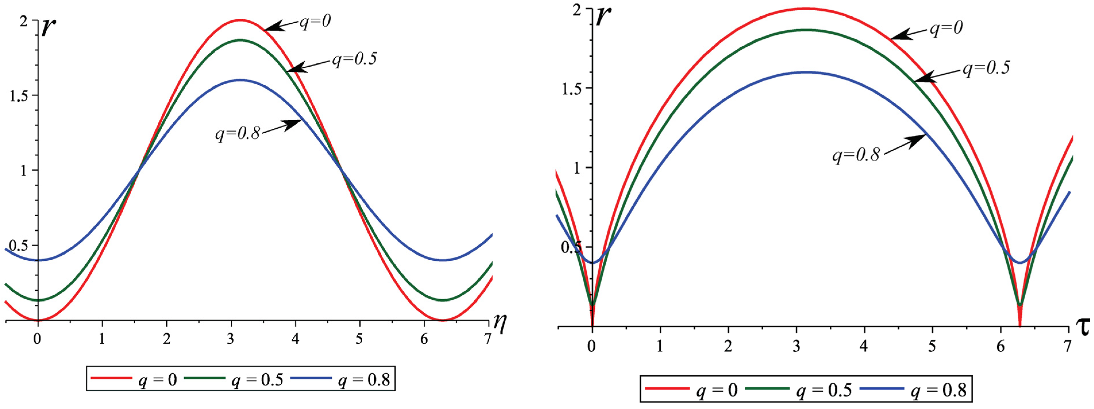
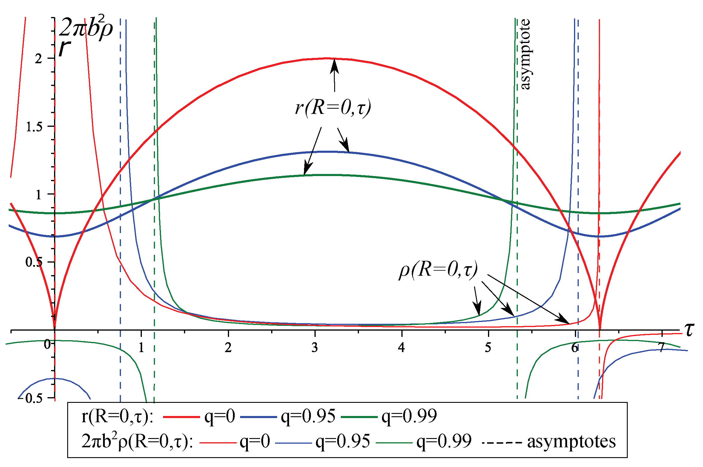
The time dependence of the throat radius $r_{\mathrm{th}}$ and the density ${\rho }_{\mathrm{th}}$ on the throat were studied in [60]. Here, for completeness, we reproduce some figures from [60]. Thus, Figure 1 shows the time dependence of the throat radius, while the density ${\rho }_{\mathrm{th}}$ is shown in Figure 2 for $k=1$ and different values of q, where dashed lines show the asymptotes of the function. Finite positive density values are observed for only a finite period of time $\eta \in ({\eta }_1,{\eta }_2)$ while $2N_2-N_1>0$, between two singularities at which $\rho$ and $\mathcal{K}$ diverge. Outside this time interval, in the case $q\ne 0$, the matter density changes its sign along with $d^{2}r/d{l}^2$, therefore the throat conditions hold together with the condition $\rho >0$.

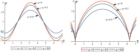
Figure 1. Time dependence of the throat radius for $q=0,0.5,0.8$ in terms of $\eta$ (left) and in terms of $\tau$ (right).

Figure 2. Time dependence of the functions $2\pi b^2\rho$ (thin lines) and $r(0,\tau )$ (thick lines) on the throat $R=0$ for $q=0,0.95,0.99$ in the model (26). Dashed lines show the asymptotes. For other values of q the plots look in a similar way.

Thus we observe a good wormhole behavior of our solution within the time interval $\eta \in ({\eta }_1,{\eta }_2)$. As the charge decreases, this interval increases; and at $q=0$, we obtain ${\eta }_1=0$, ${\eta }_2=2\pi$. Outside the throat (at $R\ne 0$), the plots look almost the same, but the singularities occur at other time instants.

5. Matching to a Dust-Filled Friedmann Universe

5.1. General Observations

Now, let us look how the wormhole solution discussed above can be inscribed into the closed Friedmann isotropic space-time characterized by the relations (12) and (13). At that, we can note [60] that to join two LTB space-time regions, characterized by different functions $F\left(R\right)$ and $h\left(R\right)$, at some hypersurface $\Sigma$ corresponding to a fixed value of the radial coordinate $R=R^{*}$, one should first of all identify $\Sigma$ as viewed from different sides. Hence, the metric tensor must be continuous on $\Sigma$. With the metric (1) it simply leads to $\left[r^2(R,\tau )\right]=0$ (as usual, square brackets denote jumps when crossing the transition surface $\Sigma$), while by (1) $g_{\tau \tau }\equiv 1$ on both sides and does not lead to any further requirements.

Next, to avoid the emergence of a shell of matter on the junction surface $\Sigma$, according to the Darmois–Israel matching conditions [85,86], one should require continuity of the second quadratic form on $\Sigma$. When applied to the metric (1), this requirement leads to $\left[{\mathrm{e}}^{-\lambda }{g}_{\tau \tau }^{\prime }\right]=0$ (which holds trivially due to $g_{\tau \tau }\equiv 1$) and $\left[{\mathrm{e}}^{-\lambda }{r}^{\prime }\right]=0$. As a result, with (7) and (11), we obtain

$$\left[r\right]=0,\left[{\mathrm{e}}^{-\lambda }{r}^{\prime }\right]=0\Rightarrow \left[h\right]=0,\left[F\right]=0.$$

(31)

Thus, to match two LTB solutions on a surface $\Sigma$ ($R=R^{*}$), it is sufficient to identify the values of $F\left(R^{*}\right)$ and $h\left(R^{*}\right)$ in these solutions. It is important that by Equation (11), the above matching conditions hold at all times at which both solutions remain regular. Also, there is no necessity to worry about the choice of the radial coordinates on different sides of $\Sigma$ because both quantities r and ${\mathrm{e}}^{-\lambda }{r}^{\prime }$ are insensitive to the choice of the coordinate R, and at reparametrizations of R the arbitrary functions $h\left(R\right)$ and $F\left(R\right)$ behave as scalars and preserve their values.

Now, let us apply the conditions (31) to the Friedmann solution (12) and (13) with $q=0$ and an arbitrary wormhole solution described above, also putting $q=0$, and let us specify the junction surface $\Sigma$ by some values of the radial coordinates $\chi ={\chi }_{\ast }$ and $R=R_{*}>0$ (here and henceforth, we mark by an asterisk the values of different quantities on $\Sigma$). We then obtain for the wormhole solution

$$h_{*}={sin}^2{\chi }_{\ast },F_{*}=2a_0{sin}^3{\chi }_{\ast }\Rightarrow F_{*}=2a_0{h}_{*}^{3/2}.$$

(32)

Consider, as before, the instant of maximum expansion, $\eta =\pi$, then $r=F/h$, and according to (32), we obtain

$$F_{*}=r_{*}{h}_{*}=2a_0{h}_{*}^{3/2}\Rightarrow h_{*}=r_{*}^2/\left(4a_0^2\right).$$

(33)

For the density, we can apply Equation (24); hence, on $\Sigma$, we have

$${\rho }_{*}{|}_{\eta =\pi }=\frac{h_{*}}{8\pi G{r}_{*}^2\left(1-r_{*}{h}_{*}^{\prime }/F_{*}^{\prime }\right)}=\frac{1}{32\pi G{a}_0^2\left(1-r_{*}{h}_{*}^{\prime }/F_{*}^{\prime }\right)}.$$

(34)

Assuming, as before, that everywhere in the wormhole solution $F^{\prime }/h^{\prime }<0$, we arrive at the inequality

$${\rho }_{*}{|}_{\eta =\pi }<\frac{1}{32\pi G{a}_0^2}\approx 5.5\times {10}^{-30}\frac{\mathrm{g}}{{\mathrm{cm}}^3}$$

(35)

if we assume $a_0\sim {10}^{28}$ cm, approximately the size of the visible part of the universe.

On the other hand, in the Friedmann solutions (12) and (13), the matter density is

$${\rho }_{\mathrm{Fr}}\left(\eta \right)=\frac{3}{4\pi G{a}_0^2{(1-cos\eta )}^3},{\rho }_{\mathrm{Fr}}{|}_{\eta =\pi }=\frac{3}{32\pi G{a}_0^2}.$$

(36)

Thus according to (35), the wormhole matter density at the junction surface $\Sigma$ is not only very small, but it is even a few times smaller (by at least a factor of three) than the cosmological matter density. In other words, the wormhole region is, at least close to $\Sigma$, a region of smaller density, maybe resembling a void. This observation was made for the instant $\eta =\pi$, but it remains true at all times since the $\eta$ dependence is the same for the wormhole and cosmological solutions.

Some more general observations can be made. As follows from the throat conditions (20), $h\left(R\right)$ has a maximum with $h=h_{\mathrm{th}}=1$, while $F\left(R\right)$ has a minimum; therefore, according to (11),

$$F\left(R\right)\ge F\left(0\right)=r_{\mathrm{th}}{|}_{\eta =\pi },$$

(37)

where, for simplicity, $h\left(R\right)$ and $F\left(R\right)$ are assumed to be monotonic in the ranges $R>0$ and $R<0$. Considering, as before, the instant of maximum expansion, $\eta =\pi$, from Equations (32) and (33), we obtain at the junction surface $R=R_{*}$:

$$F_{*}=2a_0{h}_{*}^{3/2},r_{*}{|}_{\eta =\pi }=\frac{F_{*}}{h_{*}}\Rightarrow r_{*}=F_{*}^{1/3}{\left(2a_0\right)}^{2/3},$$

(38)

Equations (37) and (38) lead to

$$\begin{array}{ccc}& & r_{*}⩾{\left(2a_0\right)}^{2/3}{r}_{\mathrm{th}}^{1/3}=7.4\times {10}^{18}{\left(\frac{r_{\mathrm{th}}}{\mathrm{cm}}\right)}^{1/3}\mathrm{cm},\hfill \end{array}$$

(39)

$$\begin{array}{ccc}& & r_{\mathrm{th}}⩽\frac{r_{*}^3}{{\left(2a_0\right)}^2}=2.5\times {10}^{-57}\frac{r_{*}^3}{{\mathrm{cm}}^3}\mathrm{cm},\hfill \end{array}$$

(40)

where $r_{\mathrm{th}}$ and $r_{*}$ are taken at maximum expansion, $\eta =\pi$. We see that the length scales of the wormhole region $r_{*}$ and its throat $r_{\mathrm{th}}$ are substantially different in cases of physical interest, $r_{*}\ll a_0$. Furthermore, the throat lifetime is $\Delta {\tau }_{\mathrm{th}}=2\pi r_{\mathrm{th}}/c$, while the lifetime of the wormhole region coincides with that of the universe, $\Delta {\tau }_{*}=2\pi a_0/c\approx 2\times {10}^{18}$ s, and thus, we have $\Delta {\tau }_{\mathrm{th}}\ll \Delta {\tau }_{*}$. All these estimates (25), (35) and (39) are based on our general assumptions about the model. Numerical estimates for a specific choice of the functions $h\left(R\right)$ and $F\left(R\right)$ will be made below.

5.2. Estimates for a Particular Model

Now, to obtain further estimates, let us describe the wormhole region by Equations (26) and (27); then, the junction conditions (31) lead to

$$R_{*}=cot{\chi }_{\ast },b=a_0{(sin{\chi }_{*})}^{3+2k},$$

(41)

which ensures matching at $R^{*}>0$. Since the functions involved in (26) are even, a similar kind of matching can be applied at $R^{*}<0$. The resulting composite model then consists of two closed evolving dust-filled Friedmann universes, connected by means of a wormhole, thus forming a dumbbell-like configuration, or otherwise, we can suppose that negative values of R lead to the same Friedmann universe at some different location.

Some numerical estimates are in order. Taking, as before, $a_0\sim {10}^{28}$ cm, let us also assume that the wormhole region is small as compared to the whole universe; hence, ${\chi }_{\ast }\ll 1$, and $sin{\chi }_{\ast }\approx {\chi }_{\ast }$. Accordingly,

$$R_{*}=1/{\chi }_{\ast },h_{*}={\chi }_{\ast }^2,F_{*}=2b{\chi }_{\ast }^{-2k},b=a_0{\chi }_{\ast }^{2k+3}.$$

(42)

Note that in the wormhole solution $r(R,\eta )=b(1+R^2)(1-cos\eta )$, and $R=0$ is the throat, so $2b$ is the maximum value of the throat radius, $2b=r(0,\pi )$.

Relationships for the wormhole parameters are easily calculated. Equations (24) and (26) imply $r{h}^{\prime }/F^{\prime }=-1/k$, and we obtain for the matter density

$$\begin{array}{ccc}& & {\rho }_{\mathrm{th}}=\frac{c^2}{32\pi G{b}^2}\frac{k}{k+1}\approx 1.3\times {10}^{26}\frac{k}{k+1}\frac{\mathrm{g}}{{\mathrm{cm}}^3}\frac{{\mathrm{cm}}^2}{b^2},\hfill \end{array}$$

(43)

$$\begin{array}{ccc}& & {\rho }_{*}=\frac{c^2}{32\pi G{a}_0^2}\frac{k}{k+1}\approx 1.3\times {10}^{-30}\frac{k}{k+1}\frac{\mathrm{g}}{{\mathrm{cm}}^3}.\hspace{1em} \hfill \end{array}$$

(44)

The junction conditions (41) imply

$$r_{*}=2a_0{\left(\frac{b}{a_0}\right)}^{1/(2k+3)}.$$

(45)

The minimum value of $r_{*}$ for given b corresponds to the limit $k\to 0$, specifically. $r_{*}⩾2a_0^{2/3}{b}^{1/3}$ (39).

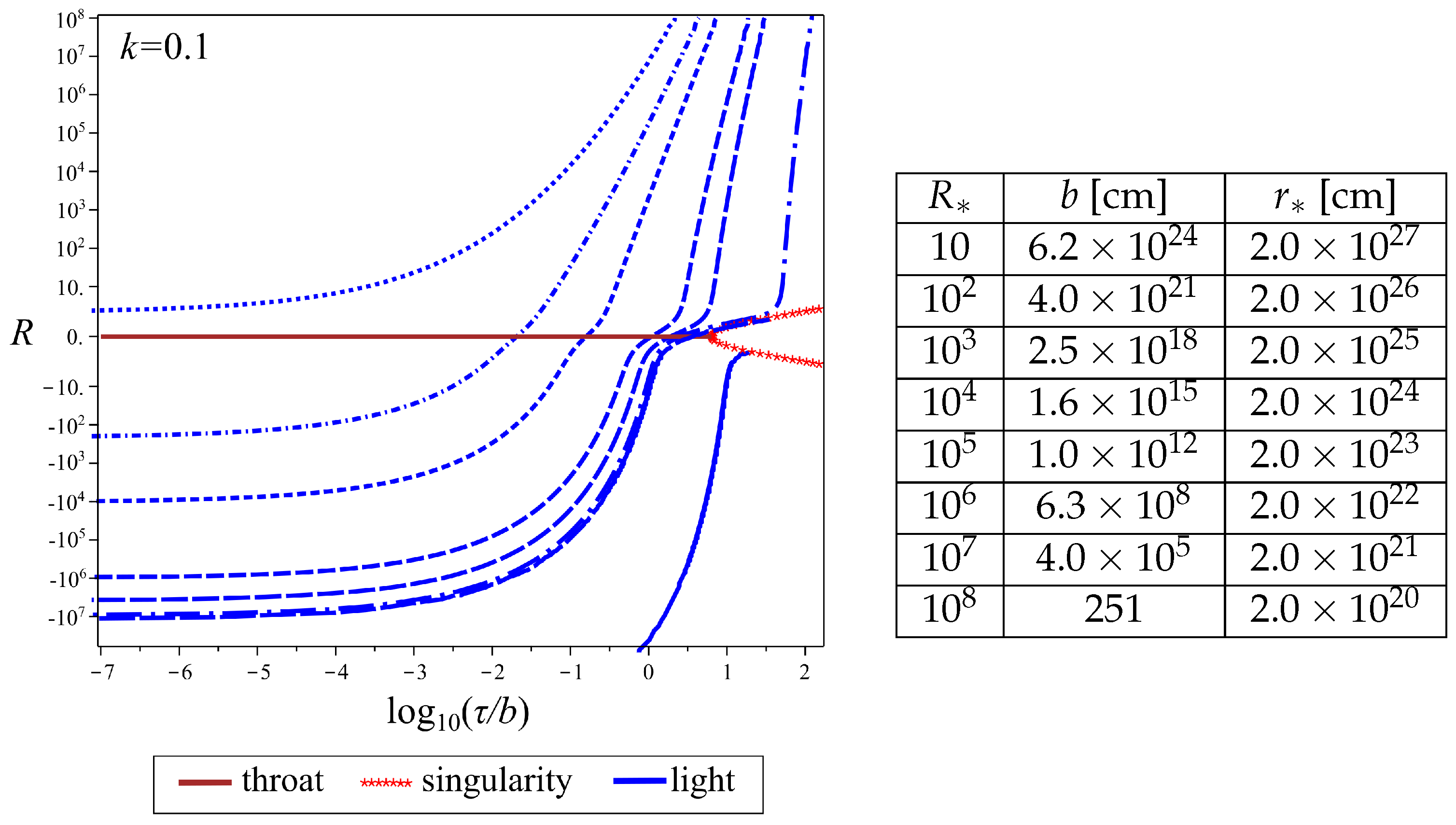
Table 1 and Table 2 show some estimates of the wormhole parameters, such as the throat radius $r_{\mathrm{th}}=2b$, matter density ${\rho }_{\mathrm{th}}$ on the throat and the radius $r_{*}$ of the whole wormhole region in the cases $k=0.1$ and $k=1$. The density at the junction surface does not depend on b and equals ${\rho }_{*}=1.2\times {10}^{-31}\mathrm{g}/{\mathrm{cm}}^3$ for $k=0.1$, and ${\rho }_{*}=6.7\times {10}^{-31}\mathrm{g}/{\mathrm{cm}}^3$ for $k=1$. We see that the wormhole region has the size of parsecs or more even for small throats. Near the throat, the density is super-nuclear for $b=1$ km, it is of white-dwarf order near a throat of planetary size, and reasonably small near a throat of 1 pc. At the junction, the density ${\rho }_{*}$ is smaller than the mean cosmological density, as should be the case according to our general observations.

Table 1. Estimates of matter density ${\rho }_{\mathrm{th}}$ at the throat and the radius $r_{*}$ of the wormhole region for different throat radii $r_{\mathrm{th}}$, in the case $k=0.1$, ${\rho }_{*}=1.2\times {10}^{-31}\mathrm{g}/{\mathrm{cm}}^3$.

${\mathit{r}}_{\mathbf{th}}$	${\mathit{r}}_{*}$	${\mathit{\rho }}_{\mathbf{th}}$$[\mathbf{g}/{\mathbf{cm}}^3]$
$1.6\times {10}^{-33}$ cm (Planck length)	$1.6\times {10}^4$ km (Earth)	$1.9\times {10}^{91}$
1 km	${10}^{21}\mathrm{cm}=338$ pc	$4.9\times {10}^{15}$ (nuclear density)
10 km (neutron star)	700 pc	$4.8\times {10}^{13}$
$6.4\times {10}^3$ km (Earth)	$5.1$ Kpc	$1.4\times {10}^8$ (white dwarf)
$2.3\times {10}^5$ km	16 Kpc (Milky Way)	$94\times {10}^3$
$695\times {10}^3$ km (Sun)	23 Kpc	${10}^4$
${10}^7$ km (super BH)	52 Kpc	49
$7\times {10}^7$ km	96 Kpc	1 (${\mathrm{H}}_2\mathrm{O}$)
1 pc	$5.7$ Mpc	$5.1\times {10}^{-12}$
$6.5$ pc	10 Mpc (galaxy cluster)	$1.9\times {10}^{-13}$
10 Kpc	100 Mpc (void)	$4.8\times {10}^{-20}$ (interstellar medium)

Table 2. Estimates of matter density ${\rho }_{\mathrm{th}}$ at the throat and the radius $r_{*}$ of the wormhole region for different throat radii $r_{\mathrm{th}}$, in the case $k=1$, ${\rho }_{*}=6.7\times {10}^{-31}\mathrm{g}/{\mathrm{cm}}^3$.

${\mathit{r}}_{\mathbf{th}}$	${\mathit{r}}_{*}$	${\mathit{\rho }}_{\mathbf{th}}$$[\mathbf{g}/{\mathbf{cm}}^3]$
$1.6\times {10}^{-33}$ cm (Planck length)	$1.2\times {10}^{11}$ km	${10}^{92}$
2 cm	16 Kpc (Milky Way)	$7\times {10}^{25}$
1 km	$0.14$ Mpc	$2.7\times {10}^{16}$ (nuclear density)
10 km (neutron star)	$0.2$ Mpc	$2.7\times {10}^{14}$
$1.6\times {10}^4$ km	1 Mpc	${10}^8$ (white dwarf)
$695\times {10}^3$ km (Sun)	$2.1$ Mpc	$5.6\times {10}^4$
${10}^7$ km (super BH)	$3.6$ Mpc	268
$1.6\times {10}^8$ km	$6.2$ Mpc	1 (${\mathrm{H}}_2\mathrm{O}$)
$1.7\times {10}^9\mathrm{km}$	10 Mpc (galaxy cluster)	$8.6\times {10}^{-3}$
1 pc	71 Mpc	$2.8\times {10}^{-11}$
$6.7$ pc	100 Mpc (void)	$8.6\times {10}^{-13}$ (interstellar medium)

6. Wormhole Lifetime and Traversability

Now, we would like to consider the radial motion of photons in the model (26) of a dust layer, assuming that it is bounded by $\left|R\right|<R_{*}$ and is located between two copies of Friedmann space-time. It is clear that a photon radially falling to such a wormhole and reaching the throat has no other way than to travel further in the direction of another universe or maybe a distant part of the same universe. The question is whether or not it will go out from the dust layer in this “other” universe rather than a singularity. In other words, whether the wormhole (or the wormhole part of space-time) is traversable.

Further on, we will consider the motion of photons under different choices of the arbitrary function ${\tau }_0\left(R\right)$ in the solution (11) with $\Delta =1$ while in the Friedmann solution we fix ${\tau }_0\equiv 0$. It should be noted here that for a particular LTB solution taken separately, the choice of ${\tau }_0\left(R\right)$ means nothing else than clock synchronization, or in other words, the choice of spatial sections of the same space-time in the same reference frame. However, in a composite model like ours, unifying two different LTB solutions, this choice is more meaningful, and different ${\tau }_0\left(R\right)$ corresponds to different synchronization of events in one region relative to events in the other region. Thus, fixing ${\tau }_0\left(R\right)\equiv 0$ in the wormhole solution, we make a physical assumption that the wormhole throat emerges simultaneously with the whole Friedmann universe, while ${\tau }_0\left(R\right)>0$ means that this happens later from the viewpoint of an observer located in this universe. We will consider both options.

6.1. Radial Motion of Photons in the Case ${\tau }_0=0$

From the metric (1), it follows for null radial geodesics that

$$\begin{array}{c}\hfill \frac{dR}{d\tau }=\pm \frac{\sqrt{1-h}}{|r^{\prime }|},\end{array}$$

(46)

where the derivative $r^{\prime }=r^{\prime }(R,\tau )$ can be found from Equation (27):

$$\begin{array}{c}\hfill r^{\prime }(R,\tau )=\frac{bR{(R^2+1)}^k}{1-cos\eta }\left[4k+5-4(k+1)cos\eta -(2k+3)\eta sin\eta -{cos}^2\eta \right].\end{array}$$

(47)

The plus sign in Equation (46) corresponds to the photon motion through the wormhole from $R<0$ to $R>0$, and the minus sign to the opposite motion. Due to the symmetry of the model, it is sufficient to consider, for example, the plus sign.

Let us calculate the time derivative of the spherical radius $r(\tau ,R(\tau \left)\right)$ along a light ray $R=R\left(\tau \right)$:

$$\begin{array}{c}\hfill \frac{d}{d\tau }r(\tau ,R\left(\tau \right))=\frac{\partial r}{\partial \tau }+\frac{\partial r}{\partial R}\frac{dR}{d\tau }=\pm \sqrt{f+\frac{F}{r}}\pm \sqrt{1-h},,\end{array}$$

(48)

where $R=R\left(\tau \right)$ describes the radial motion of a photon (46); the first ± sign corresponds to the expansion (+) of the dust shells at $\eta \in (0;\pi )$ or their contraction (−) at $\eta \in (\pi ;2\pi )$; the second ± sign corresponds to photon motion from the throat (+), or to the throat (−). It is clear that $dr/d\tau <0$ or $>0$ means convergence or divergence of light rays. Note that at the throat, $h\left(0\right)=1$, the photons move parallel to dust particles: $dr(\tau ,R(\tau \left)\right)/d\tau =\partial r/\partial \tau$.

It is instructive to define an apparent horizon as the location of turning points for radial light rays, that is, the set of events where the light rays stop diverging and start to converge, or vice versa, hence,

$$\frac{d}{d\tau }r(\tau ,R\left(\tau \right))=0.$$

(49)

Using Equations (27) and (48), Equation (49) is rewritten in the form

$$cot\frac{\eta }{2}\pm R=0,$$

(50)

and finally, we have the parametric equations for the apparent horizon

$$\begin{array}{c}\hfill r=\frac{2^{k+1}b}{{(1-cos\eta )}^k},\tau =\frac{2^{k+3/2}b(\eta -sin\eta )}{{(1-cos\eta )}^{k+3/2}}.\end{array}$$

(51)

The condition (49) can be satisfied only if the terms in Equation (50) have different signs. Thus, at the expansion stage $\eta \in (0;\pi )$, there is an apparent horizon for photons moving towards the throat ($\pm R<0$), while at the contraction stage $\eta \in (\pi ;2\pi )$, on the contrary, for photons moving from the throat ($\pm R>0$). There are actually two apparent horizons, depending on the direction of motion.

The results of numerical integration of Equations (46) or (48) are shown in Figure 3, Figure 4, Figure 5, Figure 6 and Figure 7. Figure 3 shows the set of null radial geodesics (blue curves) in the case $k=0.1$, presented in the coordinates $(R,\tau )$. The graph uses a log-10 scale for just the $\tau$ axis. The red line in the figure presents the singularity $\eta =2\pi$. There is also a singularity at the initial time $\tau \to 0$ ($\eta \to 0$), it is not presented. The photons begin their motion at the time instant with $\tau /b={10}^{-7}$, close to the origin of the universe, and move from the region $R<0$ to $R>0$ through the wormhole region. The throat $R=0$ is shown in brown and exists for a short time as compared to the universe lifetime. Some of the photons pass through the throat, others fall to the singularity instead of reaching the throat. Further on, this solution must be glued at some $R=R_{*}$ to the external Friedmann space-time, and the table on the right shows the correspondence between the parameter $R_{*}$ and the radius $r_{*}$.

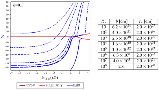
Figure 3. The figure shows the $\tau$-dependence of the radial coordinate R of photons at their radial motion (eight blue curves). The brown horizontal line presents the throat $R=0$; the red line depicts the singularity $\eta =2\pi$. The table shows the correspondence between the junction coordinate $R=R^{*}$, the throat size b, and the radius $r_{*}$ of the wormhole region. The curves from top to bottom correspond to the following initial data at the moment $\tau /b={10}^{-7}$: $R=2.3$, $-198$, $-9.7\times {10}^3$, $-9.6\times {10}^5$, $-3.7\times {10}^6$, $-1.0\times {10}^7$, $-1.1\times {10}^7$, $-1.6\times {10}^{11}$.

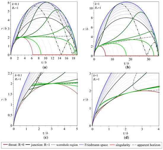
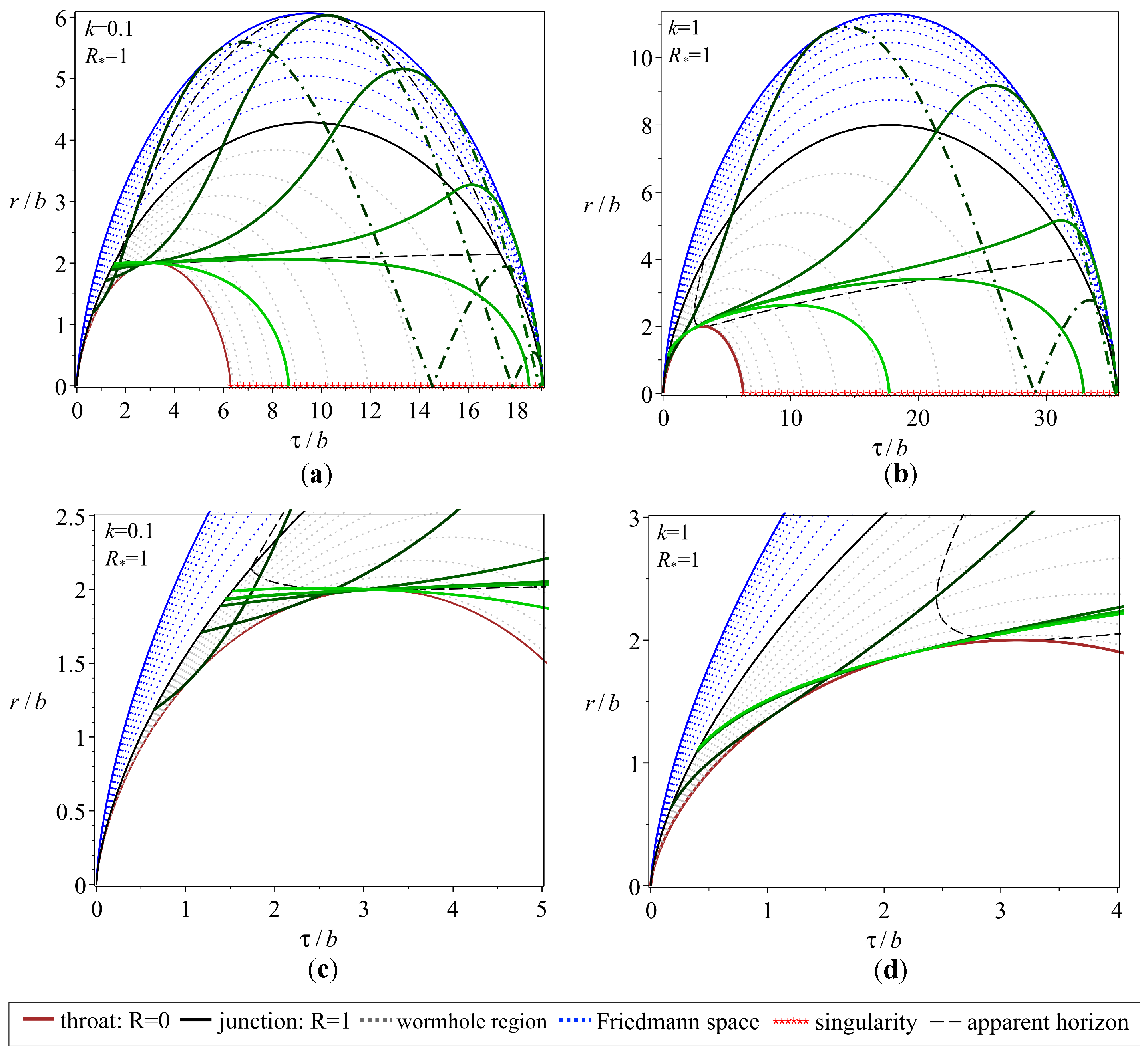
Figure 4. Illustrated are the dynamics of the throat $R=0$ (brown curve), the junction surfaces $R=\pm R_{*}$ (black curve), and dust layers of the internal wormhole region $\left|R\right|⩽R_{*}$ (black point curves) and the external Friedmann universe $\chi ⩾{\chi }_{*}$ (blue curves) in the case $R_{*}=1$. Green curves correspond to photons moving from the region $R<0$ to $R>0$. The left figures (a,c) correspond to the model with $k=0.1$; the right ones (b,d) correspond to that with $k=1$. The results are presented in two scales. The top figures (a,b) correspond to the usual scale, while the bottom figures (c,d) correspond to an enlarged scale and clarify the dynamics at early times. The photons start their motion on the sphere $R=-R_{*}$, pass through the throat, and some of them leave the wormhole region in a finite time and move further in the Friedmann space-time. The dashed-dotted green curves correspond to the motion in the region $\chi \in (\pi /2;\pi )$ of the Friedmann universe. The red line presents the singularity $r=0$, and the black dashed curve corresponds to the apparent horizon.

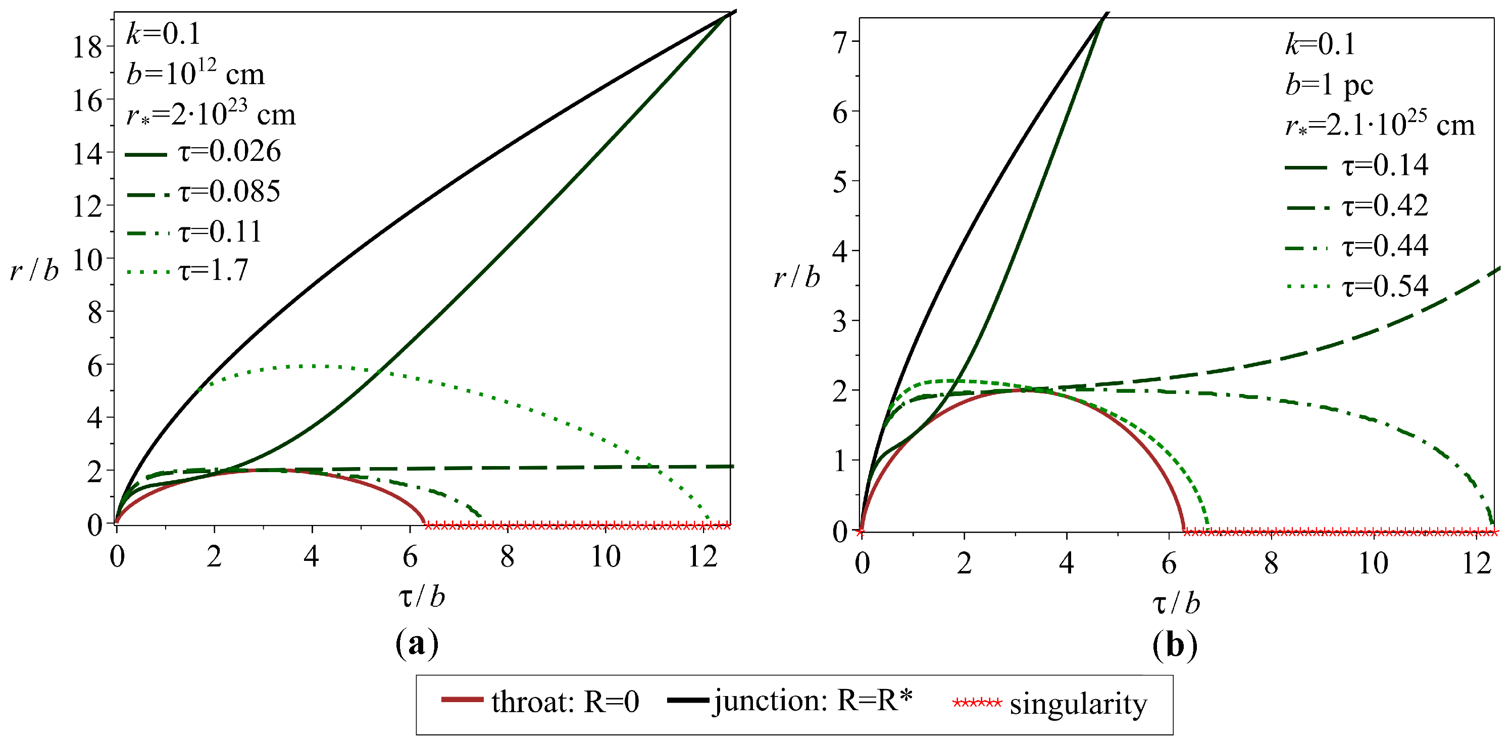
Figure 5. Dynamics of the wormhole throat $R=0$ (brown curve), the junction surface $R=\pm R_{*}$ (black curve), photon trajectories (green curves) in the cases: (a) $k=0.1$, $b={10}^{12}$ cm, $R_{*}={10}^5$, $r_{*}=2\times {10}^{23}$ cm; (b) $k=0.1$, $b=1$ pc, $R_{*}=937$, $r_{*}=2.1\times {10}^{25}$ cm. The photons are launched on the surface $R=-R_{*}$ at different times: (a) $\tau /b=0.026$, 0.085, 0.11 and 1.7; (b) $\tau /b=0.14$, 0.42, 0.44, 0.54. One of the curves does not reach the throat, the rest ones pass through the throat, and two of them reach the junction surface $R=R_{*}$.

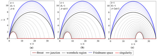
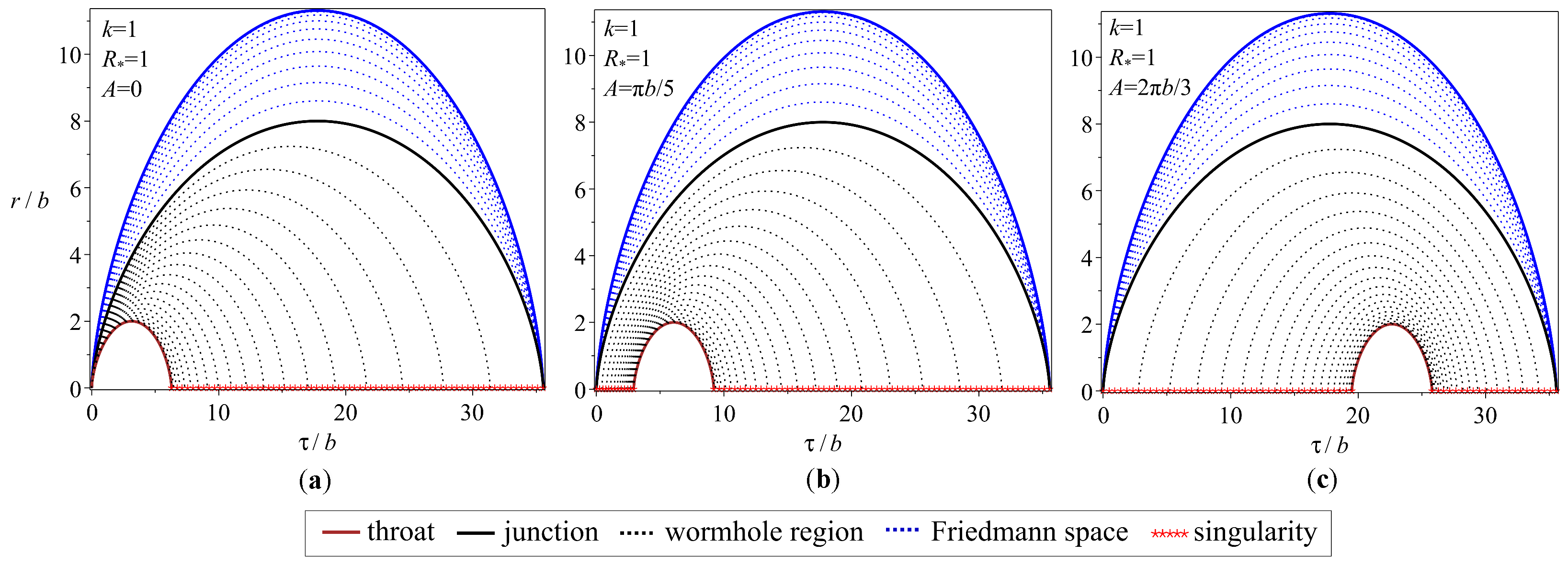
Figure 6. The figure shows the dynamics of the dust layers in the case $k=1$, $R_{*}=1$ for different values of the parameter A: (a) $A=0$, (b) $A=\pi b/5$, (c) $A=2\pi b/3$.

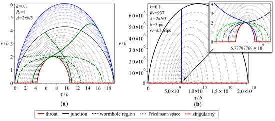
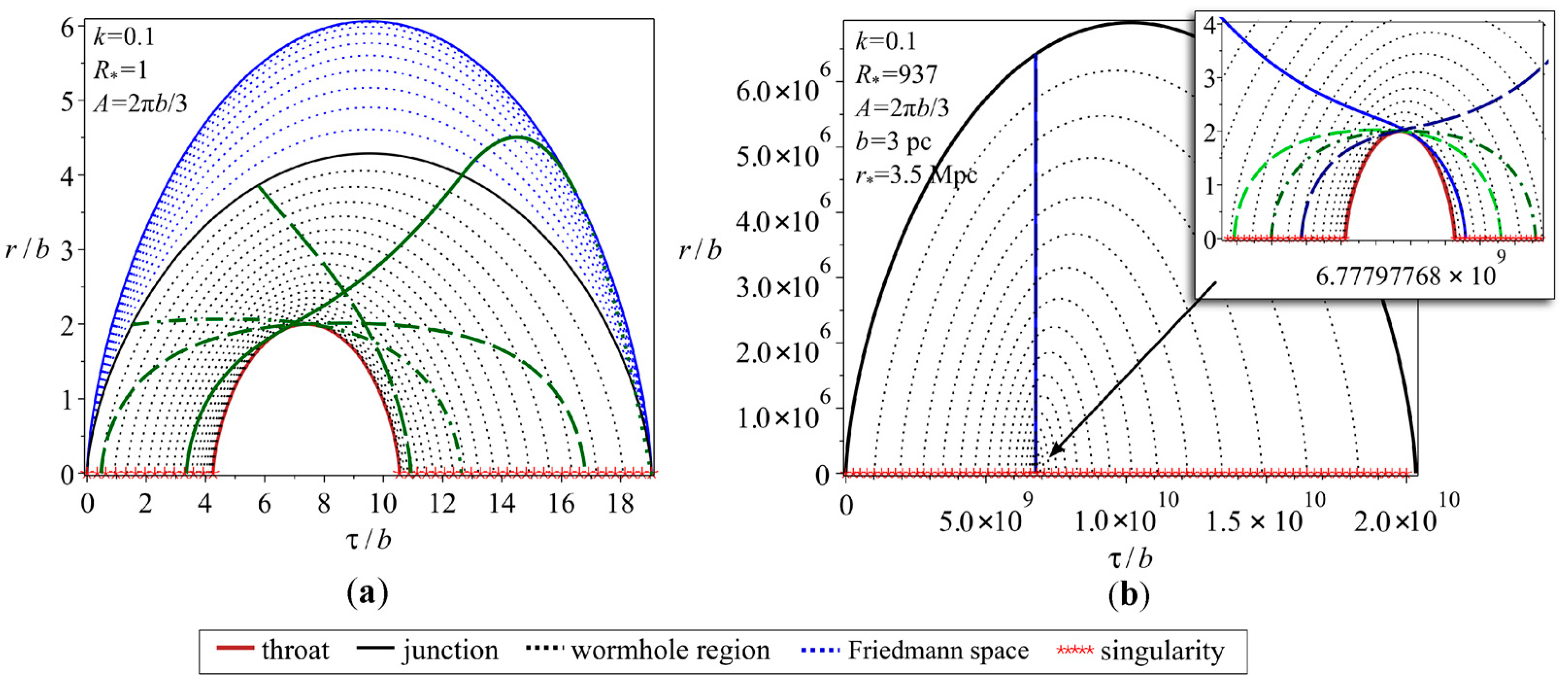
Figure 7. Dynamics of dust layers and radial photon trajectories. (a) $A=2\pi b/3$, $k=0.1$, $R_{*}=1$. (b) $A=2\pi b/3$, $k=0.1$, $R_{*}=937$, $b=3$ pc, $r_{*}=3.5$ Mpc.

Of greatest interest are large values of the parameter $R_{*}$ (see Table 1 and Table 2 above); however, for small enough $R_{*}=1$ (${\chi }_{\ast }=\pi /4$, $a_0=4\sqrt{2}b$), the results are qualitatively similar and more suitable for illustration. Figure 4 shows the dynamics of the throat $R=0$ (brown curve), dust layers of the wormhole region $\left|R\right|⩽R_{*}$ (black point curves), the junction surfaces $R=\pm R_{*}$ (black curve), external Friedmann space-time $\chi ⩾{\chi }_{\ast }$ (blue curve) in the case $R_{*}=1$, presented in the coordinates $(\tau /b,r/b)$. The left panels (a) and (c) correspond to the model with $k=0.1$; the right ones (b) and (d) correspond to that with $k=1$. The results are presented in two scales: panels (a), (b) correspond to the usual scale; (c) and (d) correspond to an enlarged scale and clarify the dynamics at early times.The green curves correspond to photons launched on the sphere $R=-R_{*}$ and moving from the region $R<0$ to $R>0$. The geodesics in the left panels (a) and (c) are results of numerical integration in the case $k=0.1$ with the following initial data at $R=-1$: $\tau /b=0.64$, $1.17$, $1.39$, $1.44$, $1.45$, $1.52$. The right panels (b) and (d) present geodesics with the following initial data at $R=-1$: $\tau /b=0.172$, $0.395$, $0.406$, $0.407$, $0.414$. The matter layers begin and end their evolution at the singularity (red line). The purple curve corresponds to the apparent horizon in the region $R>0$.

Note that to describe the motion in the $(\tau ,r)$ coordinates, in fact, a set of two diagrams is required, but due to their identity, only one of them is shown. Each diagram in the figures actually depicts two identical space-time regions $R⩽0$ and $R⩾0$, connected by the throat $R=0$.

Figure 5a,b show the time dependence of the radius $r(\tau ,R)/b$ for photon paths (green curves) with the following parameter values: (a) $k=0.1$, $b={10}^{12}$ cm, $R_{*}={10}^5$, $r_{*}=2\times {10}^{23}$ cm, and (b) $k=0.1$, $b=1$ pc, $R_{*}=937$, $r_{*}=2\times {10}^{23}$ cm, respectively. Unlike the previous figure, these values b correspond to a realistic scale of the model (see Table 1 and Table 2). The photons are launched on the junction surface $R=-R_{*}$ at different times and move from $R<0$ to $R>0$. Not all photons cross the throat and get to $R>0$, and some of them reach the junction surface $R=R_{*}$ in finite time and enter the outer space-time. In the left panel, the photons start from $R=-R_{*}$ with the initial data $\tau /b=0.026$, $0.085$, $0.11$, $1.7$. In the right panel, the photons start from $R=-R_{*}$ at the times $\tau /b=0.14$, $0.42$, $0.44$, $0.54$. For example, the value $\tau /b=0.42$ cm corresponds to the time $t=\tau b/c=1.4$ year. We can conclude that the wormhole is traversable at least during a short time of its evolution.

6.2. Radial Motion of Photons in the Case ${\tau }_0\ne 0$

Now let us consider radial null geodesics in the case (27), where ${\tau }_0\left(R\right)$ is a nonzero even function of R. The meaning of ${\tau }_0\left(R\right)$ is the time $\tau$ (by the clock of an observer in Friedmann space-time) at which the dust layer corresponding to a value of the R coordinate begins to evolve. In particular, ${\tau }_0\left(0\right)$ is the instant at which emerges the wormhole throat $R=0$; this ${\tau }_0\left(0\right)$ can take arbitrary values from the interval $0⩽{\tau }_0\left(0\right)⩽{\tau }_{max}$, where ${\tau }_{max}=\tau {|}_{\eta =2\pi ,R=R_{*}}=2\pi b{(1+R_{*}^2)}^{k+3/2}$ is the lifetime of the universe. Different dust layers must not collide; therefore we must have $r^{\prime }\ne 0$ everywhere outside the throat. This condition is sufficient for the absence of a singularity, so that the density (6) and the Kretschmann scalar (18) are finite. Let the function ${\tau }_0\left(R\right)$ vanish at the boundary $R=R_{*}$ of the wormhole region, so that it does not affect the junction conditions.

The inequality $r^{\prime }\ne 0$ is satisfied if we consider the following example of the function ${\tau }_0\left(R\right)$:

$${\tau }_0\left(R\right)=A\left[{(R_{*}^2+1)}^{k+3/2}-{(R^2+1)}^{k+3/2}\right],0⩽A⩽2\pi b.$$

(52)

The derivative $r^{\prime }$ of the function $r(R,\tau )$ has the form

$$\begin{array}{c}\hfill r^{\prime }=\frac{R{(R^2+1)}^k}{1-cos\eta }\left\{A(2k+3)sin\eta +b\left[4k+5-{cos}^2\eta -4(k+1)cos\eta -(2k+3)\eta sin\eta \right]\right\},\end{array}$$

(53)

where, as can be directly verified, the expression in curly brackets is positive; hence, the condition $r^{\prime }\ne 0$ is satisfied at $R>0$ or $R<0$, and the density $\rho$ is everywhere finite and positive.

In this model, the lifetime of the wormhole throat remains unchanged, equal to $2\pi b$, but different values of the parameter A correspond to different emergence times of the wormhole throat (Figure 6). In particular, in the case $A=0$, the throat begins to evolve simultaneously with all dust layers. If we assume $A=2\pi b$, the throat collapses simultaneously with all dust layers (such fine tuning looks quite incredible but still possible in principle). Under the condition $0<A<2\pi b$, the throat emerges and collapses at intermediate times during the lifetime of the universe. Smaller values of the parameter k correspond to a more compact wormhole region. Figure 6 corresponds to the case $R_{*}=1$ ($a_0/b=4\sqrt{2}$); however, realistic values of the parameters $a_0$ and b do not change the qualitative picture of the system dynamics.

Obviously, there are photons passing through the wormhole in the case of a thin dust region $\left|R\right|⩽R_{*}$. However, as follows from the numerical estimates in Table 1, the case of a thin dust region is of little interest. As noted in the section above, the model is traversable with ${\tau }_0\left(R\right)=0$ ($A=0$). The value $A=2\pi b$ corresponds to the case where the wormhole and the whole universe collapse simultaneously. It is quite similar to the case $A=0$, and differs only by the direction of motion; in this case, the wormhole region is always traversable, at least for photons starting at times sufficiently close to the collapse time. Due to the continuity of the equations, the traversability is also expected for A close enough to zero or $2\pi b$.

The results of our numerical analysis are shown in Figure 7 for the case $k=0.1$, $A=2\pi b/3$ in two versions. The throat emerges and collapses at some intermediate times during the universe evolution since the parameter A significantly differs from its minimum ($A=0$) and maximum ($A=2\pi b$) values. Figure 7a corresponds to small enough $R_{*}=1$; in this case the results are qualitatively similar and more suitable for illustration.

Figure 7b is obtained for values more consistent with cosmic scales, namely $b=3$ pc, $r_{*}=3.5$ Mpc, $R_{*}=937$. The inset in the right panel illustrates the behavior of the trajectories on a larger scale. In this case, there are no geodesics passing through the whole wormhole area $\left|R\right|⩽R_{*}$. However, the throat is halfway traversable; photons from the universe $R<0$ can get into the region $R>R_{*}$ if they are emitted close enough to the throat. The trajectories are shown in blue for photons passing through the throat and reaching $R=-R_{*}$ or $R=R_{*}$; the green color shows trajectories passing through the throat but not leaving the wormhole area.

As a result of our numerical analysis, we can conclude the following. In the general case, the wormhole region $\left|R\right|⩽R_{*}$ can be traversable, but only under a particular choice of the throat parameters and initial conditions. For any value of the junction surface $R_{*}$, there are always light rays passing through the wormhole, at least for A close enought to zero or $2\pi b$. If the throat emerges in the middle part of the universe lifetime, photons from the universe $R<0$ can get into the region $R>R_{*}$ if emitted close enough to the throat.

6.3. Multiple Wormholes in a Multi-Universe

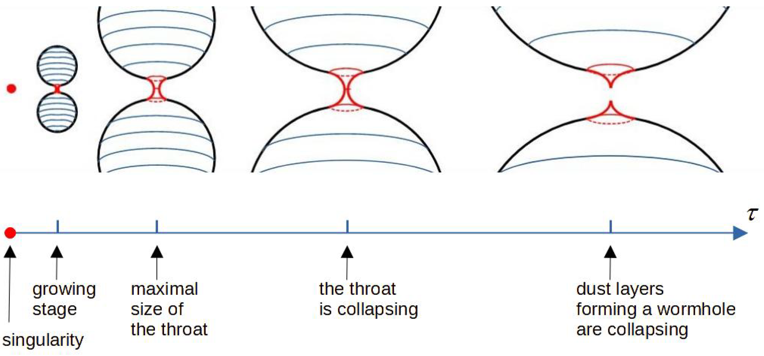
Schematically, an evolving dust-filled configuration with a wormhole connecting two closed Friedmann universes can be constructed as follows (see Figure 8). One takes two copies of such universes, cuts off from each universe a three-dimensional spherical region, and glues to the spherical boundaries being mouths of a dust-filled wormhole. This configuration evolves synchronously with the proper cosmic time $\tau$, which is supposed to be the same in all regions, from the initial cosmological singularity to the final one. It is worth noting that the wormhole mouths inscribed into closed Friedmann universes are existing in the entire cosmological cycle and evolving synchronously with the universe’s evolution, i.e., growing at the expansion phase and shrinking at contraction. On the other hand, the wormhole throat situated between the two mouths is only open during a small interval of the universe’s evolution. Figure 8 shows an example where a throat appears at the moment of initial singularity, then it grows, achieves its maximum size, and after that, it shrinks and disappears. In Figure 6, one can see other examples where wormhole throats appear during cosmological evolution.

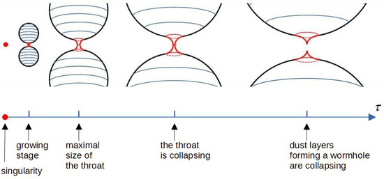
Figure 8. An evolving wormhole connecting two Friedmann universes.

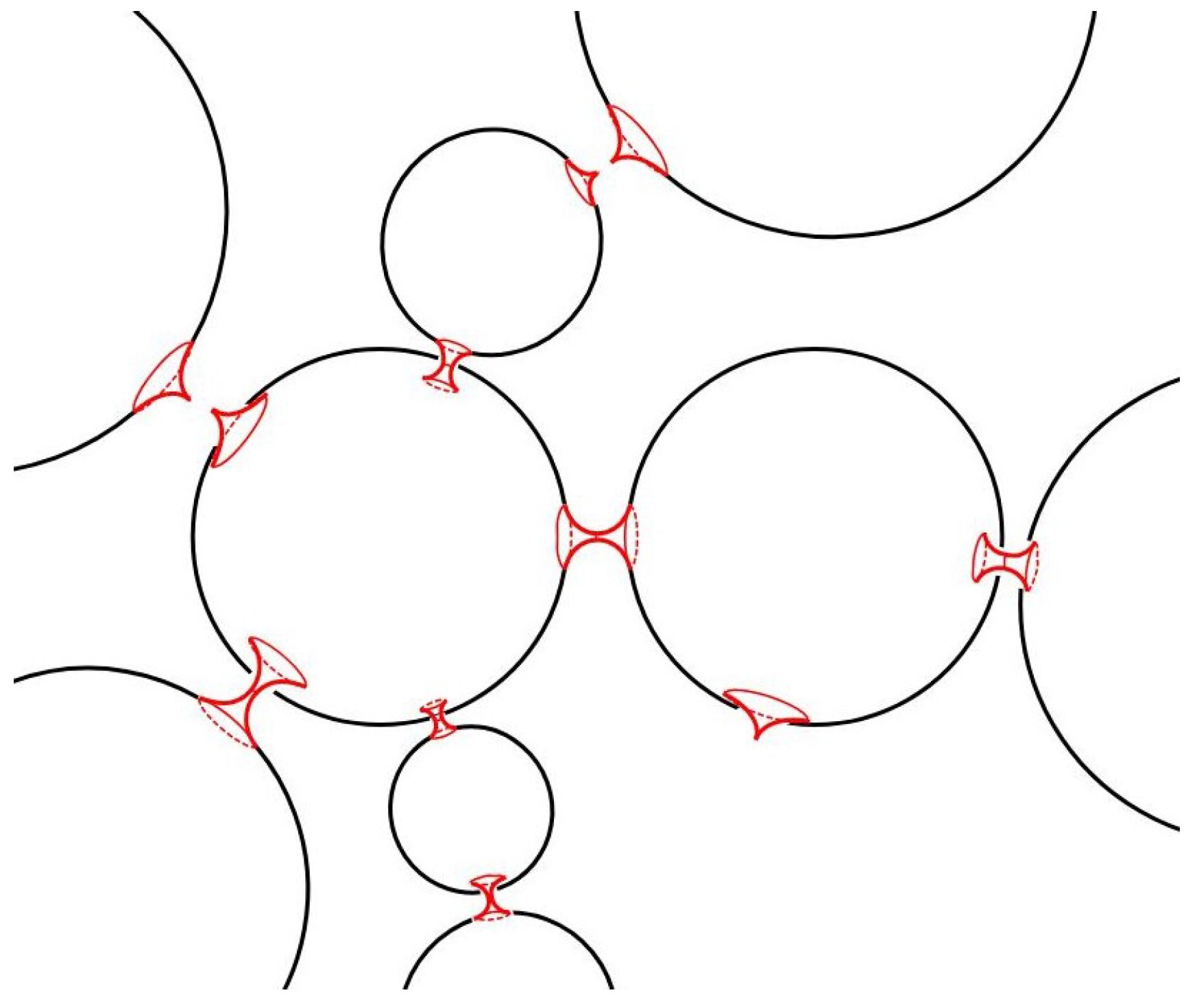
The model with one dust-filled wormhole connecting two closed Friedmann universes can be naturally generalized. We can suppose that the “mother” Friedmann universe is born with multiple mouths of wormholes associated to “daughter” universes. As a result, we obtain a model of a multi-universe as a system of closed Friedmann universes connected by evolving dust-filled wormholes (see Figure 9).

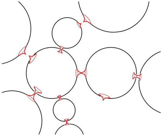
Figure 9. Multiple wormholes in the multi-universe.

Here it is necessary to stress once more that the multi-universe with multiple wormholes evolves synchronously with unified proper cosmic time $\tau$, which is supposed to be the same in all regions. Such a high correlation between different regions can be explained if one supposes that the multi-universe is born from the quantum spacetime foam on sub-Planckian scales as a single quantum state.

One more point worth being stressed is the following. Strictly speaking, the Friedmann universe with an inscribed wormhole mouth is already neither homogeneous nor isotropic. A distant observer will see a wormhole mouth as a compact object bending photon trajectories. In addition, a wormhole mouth will introduce distortions into the spectrum of the almost isotropic cosmic microwave background radiation. The scale of anisotropy must be proportional to an angular size of the mouth. In principle, these both effects could be potentially observable, therefore, one might verify the model of dust-filled wormholes in the Friedmann universe using astrophysical methods. Particular predictions of this kind require a further study.

7. Concluding Remarks

In this paper, we have continued our study begun in [60] and described in some detail different features of evolving wormholes able to exist in a Friedmann universe in the simplest case of purely dust solutions. However, it is evident that adding small values of the cosmological constant $\mathsf{\Lambda }$ cannot qualitatively change such local issues as the existence and properties of wormholes. Meanwhile, a nonzero $\mathsf{\Lambda }$ drastically changes the global dynamics: $\mathsf{\Lambda }>0$ launches a stage of accelerated expansion of the Universe, which must probably encompass the wormhole region. It is important that such wormhole regions can exist not only at a matter-dominated stage of the Universe evolution but also at its accelerated stage. In particular, examples of solutions to the Einstein equations describing wormholes in a de Sitter universe are known, and it has been noticed that such wormholes, if they existed at an inflationary stage, could greatly extend the causal connection of different parts of the universe [23].

On the other hand, the inclusion of a sufficiently small charge $q\ne 0$ also cannot strongly change the local picture of a wormhole. However, globally, the Universe cannot be precisely homogeneous and isotropic in the presence of a vector field. Also, a charge (or an effective charge due to a wormhole) on one “pole” inevitably leads to an opposite charge on the other, where the lines of force again converge. There can be a similar wormhole mouth at this other pole and one more universe beyond it, and so on. The whole picture will resemble a “churchkhela,” wonderful Georgian dessert, see Figure 10. As before, there can also be natural generalizations in the spirit of Figure 9, not to mention that some of the wormholes may connect different parts of the same universe. Possible observational signatures of such objects, in particular, concerning the properties of cosmic microwave background and cosmic magnetic fields, can be a subject of further studies. It may be of particular interest to compare the characteristics of our wormhole models with the observed parameters of cosmic voids and other local inhomogeneities in our universe.

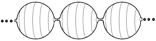
Figure 10. Multiple universes connected by magnetic wormholes.

References

- Friedman, A. Über die Krümmung des Raumes. Z. Phys. 1922, 10, 377–386. [Google Scholar] [CrossRef]
- Flamm, L. Beitrage zur Einsteinschen Gravitationstheorie. Phys. Z. 1916, 17, 448. [Google Scholar]
- Einstein, A.; Rosen, N. The particle problem in the General Theory of Relativity. Phys. Rev. 1935, 48, 73–77. [Google Scholar] [CrossRef]
- Wheeler, J.A. Geons. Phys. Rev. 1955, 97, 511–536. [Google Scholar] [CrossRef]
- Wheeler, J.A. Geometrodynamics; Academic Press: New York, NY, USA, 1962; 334p. [Google Scholar]
- Bronnikov, K.A. Scalar-tensor theory and scalar charge. Acta Phys. Pol. B 1973, 4, 251. [Google Scholar]
- Ellis, H.G. Ether flow through a drainhole—A particle model in general relativity. J. Math. Phys. 1973, 14, 104–118. [Google Scholar] [CrossRef]
- Ellis, H.G. The evolving, flowless drainhole: A nongravitating-particle model in general relativity theory. Gen. Relat. Gravit. 1979, 10, 105–123. [Google Scholar]
- Clément, G. A class of wormhole solutions to higher dimensional general relativity. Gen. Rel. Grav. 1984, 16, 131–138. [Google Scholar] [CrossRef]
- Clément, G. Axisymmetric regular multiwormhole solutions in five-dimensional general relativity. Gen. Rel. Grav. 1984, 16, 477–489. [Google Scholar] [CrossRef]
- Morris, M.S.; Thorne, K.S. Wormholes in spacetime and their use for interstellar travel: A tool for teaching general relativity. Am. J. Phys. 1988, 56, 395. [Google Scholar] [CrossRef]
- Bronnikov, K.A. Spherically symmetric solutions in D-dimensional dilaton gravity. Grav. Cosmol. 1995, 1, 67–78. [Google Scholar]
- Clément, G.; Fabris, J.C.; Rodrigues, M.E. Phantom black holes in Einstein-Maxwell-dilaton theory. Phys. Rev. D 2009, 79, 064021. [Google Scholar] [CrossRef]
- Goulart, P. Phantom wormholes in Einstein-Maxwell-dilaton theory. Class. Quantum Grav. 2017, 35, 025012. [Google Scholar] [CrossRef]
- Huang, H.; Yang, J. Charged Ellis wormhole and black bounce. Phys. Rev. D. 2019, 100, 124063. [Google Scholar] [CrossRef]
- Lobo, F.S.N. Chaplygin traversable wormholes. Phys. Rev. D 2006, 73, 064028. [Google Scholar] [CrossRef]
- Sushkov, S.V. Wormholes supported by a phantom energy. Phys. Rev. D 2005, 71, 043520. [Google Scholar] [CrossRef]
- Kuhfittig, P.K.F. Conformal-symmetry wormholes supported by a perfect fluid. New Horizons Math. Phys. 2017, 1, 14–18. [Google Scholar] [CrossRef]
- Lobo, F.S.N. Stable phantom energy traversable wormhole models. AIP Conf. Proc. 2006, 861, 936–943. [Google Scholar]
- Kuhfittig, P.K.F. Exactly solvable wormhole and cosmological models with a barotropic equation of state. Acta Phys. Pol. B 2016, 47, 1263–1272. [Google Scholar] [CrossRef]
- Sahoo, P.K.; Moraes, P.H.R.S.; Sahoo, P.G.R. Phantom fluid supporting traversable wormholes in alternative gravity with extra material terms. Int. J. Mod. Phys. D 2018, 27, 1950004. [Google Scholar] [CrossRef]
- Kuhfittig, P.K.F. Static and dynamic traversable wormhole geometries satisfying the Ford-Roman constraints. Phys. Rev. D 2002, 66, 024015. [Google Scholar] [CrossRef]
- Bronnikov, K.A.; Baleevskikh, K.A.; Skvortsova, M.V. Wormholes with fluid sources: A no-go theorem and new examples. Phys. Rev. D 2017, 96, 124039. [Google Scholar] [CrossRef]
- Visser, M. Traversable wormholes: Some simple examples. Phys. Rev. D 1989, 39, 3182. [Google Scholar] [CrossRef]
- Visser, M. Traversable wormholes from surgically modified Schwarzschild spacetimes. Nucl. Phys. B 1989, 328, 203–212. [Google Scholar] [CrossRef]
- Blázquez-Salcedo, J.L.; Knoll, C.; Radu, E. Traversable wormholes in Einstein-Dirac-Maxwell theory. Phys. Rev. Lett. 2021, 126, 101102. [Google Scholar] [CrossRef]
- Konoplya, R.A.; Zhidenko, A. Traversable wormholes in general relativity without exotic matter. Phys. Rev. Lett. 2022, 128, 091104. [Google Scholar] [CrossRef]
- Bolokhov, S.V.; Bronnikov, K.A.; Krasnikov, S.V.; Skvortsova, M.V. A note on “Traversable wormholes in Einstein-Dirac-Maxwell theory”. Grav. Cosmol. 2021, 27, 401. [Google Scholar] [CrossRef]
- Hochberg, D.; Visser, M. Geometric structure of the generic static traversable wormhole throat. Phys. Rev. D 1997, 56, 4745. [Google Scholar] [CrossRef]
- Bronnikov, K.A.; Starobinsky, A.A. No realistic wormholes from ghost-free scalar-tensor phantom dark energy. JETP Lett. 2007, 85, 1–5. [Google Scholar] [CrossRef]
- Alencar, G.; Nilton, M. Schwarzschild-like wormholes in asymptotically safe gravity. Universe 2021, 7, 332. [Google Scholar] [CrossRef]
- Bronnikov, K.A.; Kim, S.-W. Possible wormholes in a brane world. Phys. Rev. D 2003, 67, 064027. [Google Scholar] [CrossRef]
- Harko, T.; Lobo, F.S.N.; Mak, M.K.; Sushkov, S.V. Modified-gravity wormholes without exotic matter. Phys. Rev. D 2013, 87, 067504. [Google Scholar] [CrossRef]
- Mustafa, G.; Maurya, S.K.; Saibal, R. On the possibility of generalized wormhole formation in the galactic halo due to dark matter using the observational data within the matter coupling gravity formalism. Astroph. J. 2022, 941, 170. [Google Scholar] [CrossRef]
- Mustafa, G.; Hussain, I.; Atamurotov, F.; Liu, W.M. Imprints of dark matter on wormhole geometry in modified teleparallel gravity. Eur. Phys. J. Plus 2023, 138, 166. [Google Scholar] [CrossRef]
- Bronnikov, K.A.; Krechet, V.G. Potentially observable cylindrical wormholes without exotic matter in GR. Phys. Rev. D 2019, 99, 084051. [Google Scholar] [CrossRef]
- Bolokhov, S.V.; Bronnikov, K.A.; Skvortsova, M.V. Cylindrical wormholes: A search for viable phantom-free models in GR. Int. J. Mod. Phys. D 2019, 28, 1941008. [Google Scholar]
- Bronnikov, K.A.; Krechet, V.G.; Oshurko, V.B. Rotating Melvin-like universes and wormholes in general relativity. Symmetry 2020, 12, 1306. [Google Scholar] [CrossRef]
- Bronnikov, K.A.; Galiakhmetov, A.M. Wormholes and black universes without phantom fields in Einstein-Cartan theory. Phys. Rev. D 2016, 94, 124006. [Google Scholar] [CrossRef]
- Matos, T.; Miranda, G. Exact rotating magnetic traversable wormhole satisfying the energy conditions. Phys. Rev. D 2019, 99, 124045. [Google Scholar]
- Kashargin, P.E.; Sushkov, S.V. Slowly rotating scalar field wormholes: The second order approximation. Phys. Rev. D 2008, 78, 064071. [Google Scholar] [CrossRef]
- Kleihaus, B.; Kunz, J. Rotating Ellis wormholes in four dimensions. Phys. Rev. D 2014, 90, 121503. [Google Scholar] [CrossRef]
- Chew, X.Y.; Kleihaus, B.; Kunz, J. Geometry of spinning Ellis wormholes. Phys. Rev. D 2016, 94, 104031. [Google Scholar] [CrossRef]
- Arellano, A.V.B.; Lobo, F.S.N. Evolving wormhole geometries within nonlinear electrodynamics. Class. Quant. Grav. 2006, 23, 5811–5824. [Google Scholar] [CrossRef]
- Bronnikov, K.A. Nonlinear electrodynamics, regular black holes and wormholes. Int. J. Mod. Phys. D 2018, 27, 184105. [Google Scholar] [CrossRef]
- Kar, S. Evolving wormholes and the energy conditions. Phys. Rev. D 1994, 49, 862. [Google Scholar] [CrossRef]
- Kim, S.W. Cosmological model with a traversable wormhole. Phys. Rev. D 1996, 53, 6889. [Google Scholar] [CrossRef]
- Roman, T.A. Inflating Lorentzian wormholes. Phys. Rev. D 1993, 47, 1370–1379. [Google Scholar] [CrossRef]
- Sushkov, S.V.; Kim, S.W. Cosmological evolution of a ghost scalar field. Gen. Relativ. Gravit. 2004, 36, 1671–1678. [Google Scholar] [CrossRef]
- Sushkov, S.V.; Zhang, Y.Z. Scalar wormholes in cosmological setting and their instability. Phys. Rev. D 2008, 77, 024042. [Google Scholar] [CrossRef]
- Wang, A.; Letelier, P.S. Dynamic wormholes and energy conditions. Prog. Theor. Phys. 1995, 94, 137–142. [Google Scholar] [CrossRef]
- Yang, J.; Huang, H. Trapping horizons of the evolving charged wormhole and black bounce. Phys. Rev. D 2021, 104, 084005. [Google Scholar] [CrossRef]
- Hayward, S.A. Dynamic wormholes. Int. J. Mod. Phys. D 1999, 8, 373–382. [Google Scholar] [CrossRef]
- Hayward, S.A. Wormhole dynamics in spherical symmetry. Phys. Rev. D 2009, 79, 124001. [Google Scholar] [CrossRef]
- Hochberg, D.; Visser, M. Dynamic wormholes, anti-trapped surfaces, and energy conditions. Phys. Rev. D 1998, 58, 04402. [Google Scholar] [CrossRef]
- Visser, M. Lorentzian Wormholes: From Einstein to Hawking; American Institute of Physics: Woodbury, NY, USA, 1995; 412p. [Google Scholar]
- Lobo, F.S.N. Exotic solutions in General Relativity: Traversable wormholes and <<warp drive>> spacetimes. In Classical and Quantum Gravity Research; Nova Science Publishers: New York, NY, USA, 2008; pp. 1–78. [Google Scholar]
- Bronnikov, K.A.; Sushkov, S.V. Current problems and recent advances in wormhole physics. Universe 2023, 9, 81. [Google Scholar] [CrossRef]
- Kashargin, P.; Sushkov, S. Collapsing wormholes sustained by dustlike matter. Universe 2020, 6, 186. [Google Scholar] [CrossRef]
- Bronnikov, K.A.; Kashargin, P.E.; Sushkov, S.V. Magnetized dusty black holes and wormholes. Universe 2021, 7, 419. [Google Scholar] [CrossRef]
- Tolman, R. Effect of inhomogeneity on cosmological models. Proc. Natl. Acad. Sci. USA 1934, 20, 169–176. [Google Scholar] [CrossRef] [PubMed]
- Lemaître, G. L’Univers en expansion. Ann. SociÉtÉ Sci. Brux. 1933, A53, 51–85. [Google Scholar]
- Bondi, H. Spherically symmetrical models in general relativity. Mon. Not. R. Astron. Soc. 1947, 107, 410, reprinted: Gen. Rel. Grav., 1999, 31, 1783–1805. [Google Scholar] [CrossRef]
- Christodoulou, D. Violation of cosmic censorship in the gravitational collapse of a dust cloud. Commun. Math. Phys. 1984, 93, 171–195. [Google Scholar] [CrossRef]
- Landau, L.D.; Lifshitz, E.M. The Classical Theory of Fields, 4th ed.; Butterworth-Heinemann: Oxford, UK, 1987; Volume 2, 402p. [Google Scholar]
- Bambi, C. Black Holes: A Laboratory for Testing Strong Gravity; Springer Nature Singapore Pte Ltd.: Singapore, 2017; 355p. [Google Scholar]
- Markov, M.A.; Frolov, V.P. Metrics of the closed Friedman world perturbed by electric charge (to the theory of electromagnetic <<Friedmons>>). Teor. Mat. Fiz. 1970, 3, 3–17. [Google Scholar]
- Bailyn, M. Oscillatory behavior of charge-matter fluids with e/m > G1/2. Phys. Rev. D 1973, 8, 1036. [Google Scholar] [CrossRef]
- Vickers, P.A. Charged dust spheres in general relativity. Ann. Inst. Henri Poincaré A 1973, 18, 137. [Google Scholar]
- Ivanenko, D.D.; Krechet, V.G.; Lapchinskii, V.G. The dynamics of charged dust in the general theory of relativity. Sov. Phys. J. 1973, 16, 1675–1679. [Google Scholar] [CrossRef]
- Khlestkov, Y.A. Three types of solutions of the Einstein-Maxwell equations. J. Exp. Teor. Fis. 1975, 41, 188. [Google Scholar]
- Shikin, I.S. An investigation of a class of gravitational fields for a charged dustlike medium. J. Exp. Teor. Fis. 1975, 40, 215. [Google Scholar]
- Pavlov, N.V. Charged dust spheres in the general theory of relativity I. Quadratures of Einstein’s equations. Sov. Phys. J. 1976, 19, 489–495. [Google Scholar] [CrossRef]
- Pavlov, N.V.; Bronnikov, K.A. Charged dust spheres in the general theory of relativity II. Singularities and physically permissible models. Sov. Phys. J. 1976, 19, 916–920. [Google Scholar] [CrossRef]
- Bronnikov, K.A.; Kovalchuk, M.A. Some exact models for nonspherical collapse, I. Gen. Rel. Grav. 1983, 15, 809–822. [Google Scholar] [CrossRef]
- Bronnikov, K.A. Some exact models for nonspherical collapse, II. Gen. Rel. Grav. 1983, 15, 823–836. [Google Scholar] [CrossRef]
- Bronnikov, K.A.; Kovalchuk, M.A. Some exact models for nonspherical collapse, III. Gen. Rel. Grav. 1984, 16, 15–31. [Google Scholar] [CrossRef]
- Shatskiy, A.A.; Novikov, I.D.; Kardashev, N.S. A dynamic model of the wormhole and the Multiverse model. Uspekhi Fiz. Nauk. 2008, 178, 481–488. [Google Scholar] [CrossRef]
- Khlestkov, Y.A.; Sukhanova, L.A. Internal structure of wormholes—Geometric images of charged particles in general relativity. Grav. Cosmol. 2018, 24, 360–370. [Google Scholar] [CrossRef]
- Maeda, H.; Harada, T.; Carr, B.J. Cosmological wormholes. Phys. Rev. D 2009, 79, 044034. [Google Scholar] [CrossRef]
- Tomikawa, Y.; Izumi, K.; Shiromizu, T. New definition of a wormhole throat. Phys. Rev. D 2015, 91, 104008. [Google Scholar] [CrossRef]
- Bittencourt, E.; Klippert, R.; Santos, G. Dynamical wormhole definitions confronted. Class. Quantum Grav. 2018, 35, 155009. [Google Scholar] [CrossRef]
- Reissner, H. Über die Eigengravitation des elektrischen Feldes nach der einsteinschen Theorie. Ann. Der Phys. 1916, 355, 106–120. [Google Scholar] [CrossRef]
- Nordström, G. On the energy of the gravitational field in Einstein’s theory. Proc. Kon. Ned. Akad. Wet. 1918, 20, 1238–1245. [Google Scholar]
- Darmois, G. Les équations de la gravitation einsteinienne. In Mémorial des Sciences Mathematiques; Gauthier-Villars: Paris, France, 1927; p. 58. [Google Scholar]
- Israel, W. Singular hypersurfaces and thin shells in general relativity. Nuovo Cim. B 1967, 48, 463. [Google Scholar] [CrossRef]
Disclaimer/Publisher’s Note: The statements, opinions and data contained in all publications are solely those of the individual author(s) and contributor(s) and not of MDPI and/or the editor(s). MDPI and/or the editor(s) disclaim responsibility for any injury to people or property resulting from any ideas, methods, instructions or products referred to in the content. |
© 2023 by the authors. Licensee MDPI, Basel, Switzerland. This article is an open access article distributed under the terms and conditions of the Creative Commons Attribution (CC BY) license (https://creativecommons.org/licenses/by/4.0/).