1. Introduction
The Earth’s magnetopause, as the interface between the Earth’s magnetospheric plasma and solar-wind plasma, is a critical region responsible for the transfer of energy and particles between the solar wind and the magnetosphere. During the southward IMF, magnetic reconnection at the dayside magnetopause plays a significant role in the plasma entry [
1]. For the northward IMF, while reconnection at low latitude is less efficient, the Kelvin–Helmholtz instability (KHI) is one of the primary mechanisms for energy transport at the low-latitude magnetopause [
2,
3,
4,
5]. A large number of observational evidences indicate that the KH waves and vortices widely exist at the magnetopause and the inner boundary-layer surface [
6,
7,
8]. The evidence of solar-wind transport across the magnetopause through the rolled-up KH vortices was reported by Hasegawa et al. [
9], who used the observations from Cluster spacecraft near the flank magnetopause and showed that the vortices can cause solar-wind transport under the northward IMF. Later, the criteria of identifying the rolled-up KH for the single-point observation was proposed by Hasegawa et al. [
10], suggesting that the existence of low-density and high-speed magnetospheric plasma can be considered as a feature of rolled-up vortices. In the same year, Takagi et al. [
11] also established similar criteria in vortex evolution using three-dimensional magnetohydrodynamic (MHD) simulations.
KH waves have been observed under different IMF conditions and locations. Hasegawa et al. [
10] collected a number of rolled-up KH vortices in the flank magnetopause under the northward IMF using the observations from the Geotail spacecraft. Later on, using the same methodology, Taylor et al. [
12] found 17 rolled-up vortices observed by the Double Star TC-1 satellite, and they demonstrated that the location of vortices shows a clear dawn–dusk asymmetry. In the recent research of Wang et al. [
13], a sharp and transient mesoscale fluctuation of plasma and magnetic field under a long interval of northward IMF located at x ≈ 60 R
E was found. They simulated this event using the MHD model and showed that these fluctuations are KH waves in the midmagnetotail, and that the KH protrusions can influence the tail structure. Subsequently, KH waves in the midmagnetotail were also found using ARTEMIS observations in Ling et al. [
14]. They compared the KH waves in the lunar orbit and near-Earth space observed at the same time and indicated that when the KH waves flow toward the magnetotail, the phase velocity and spatial scale of KH waves increase. Although it has generally been accepted that KH waves usually occur under the northward IMF, KH waves can also occur under the southward IMF. Hwang et al. [
15] first reported in situ observation of KH waves in the nonlinear phase during the southward IMF, and demonstrated that KH waves under the southward IMF are characterized by irregularity and intermittence. After that, Yan et al. [
16] also presented KH waves at the duskside magnetopause under the southward IMF, and estimated the vorticity and the propagation velocity of the vortices. Recently, similar KH wave signatures were observed at the dusk-flank magnetopause during the southward IMF by the MMS spacecraft [
17,
18,
19]. The first KH-wave event observed by MMS during the southward IMF was reported by Blasl et al. [
18], which also showed the irregular and intermittent structures of the KH waves as in Hwang et al. [
15], as well as smaller-scale lower-hybrid (LH) waves within the primary KH waves. Nakamura et al. [
19] employed the fully kinetic simulations modeling this MMS event and proposed that the irregular and intermittent structures can be caused by the secondary Rayleigh–Taylor instability enhanced by the primary KH waves. Blasl et al. [
18] and Nakamura et al. [
19] also showed that the observed LH waves are caused by the lower-hybrid drift instability (LHDI) induced by the enhanced density jump at the edges of the primary KH waves. In addition, Nakamura et al. [
17] showed that the secondary LHDI at the vortex edges can cause an efficient solar-wind transport across the magnetopause even during the southward IMF. The vortices can also occur under the radial IMF. Farrugia et al. [
20] presented a line of vortices lasting for about 1.5 h at the flank magnetopause under the near radial IMF. Later on, Grygorov et al. [
21] showed a rolled-up vortex excited by the large-velocity shear at the inner edge of low-latitude boundary layer at the dayside magnetopause. Hwang et al. [
22] reported KH waves observed by the Cluster spacecraft under the strongly dawnward IMF, and this was the first in situ observation of KH waves along the high-latitude magnetopause near the northern duskward cusp. More KH waves at high latitude were presented by Ma et al. [
23]. Furthermore, the occurrence rate of KH-wave events has been statistically studied using magnetopause crossings from the THEMIS spacecraft located in the dayside and flank of the magnetopause for seven years by Kavosi and Raeder [
24]. They found that KH waves occur at around 19% of the magnetopause crossings despite the solar-wind conditions. The occurrence rate is around 35% of the time for the northward IMF and 10% of the time under the southward IMF. They also indicated that the occurrence rate increased with the increasing IMF cone angle, solar wind Alfvén Mach number, and density, but the IMF magnitude has a very small impact. However, there has been no report about the KH waves under southward IMF at the lunar-orbit magnetopause.
In this study, we report KH waves under the southward IMF at the lunar-orbit magnetopause. The paper is organized as follows: In
Section 2 we present the introduction of the ARTEMIS satellite and the measurements used in this study, and the KH-wave event observed by the ARTEMIS satellite at near-moon orbit. The discussion is presented in
Section 3, and
Section 4 provides a summary.
2. Observation
THEMIS was launched on 17 February 2007 and contained five identical probes (THA, THB, THC, THD, THE). The two probes of the THEMIS spacecraft, THEMIS B and THEMIS C, were captured into lunar orbit and formed the ARTEMIS (P1 and P2) mission in 2010. For the KH waves, we use the observations from the ARTEMIS mission. In this study, we use the magnetic field data from the fluxgate magnetometer (FGM) [
25] and the ion data from the electrostatic analyzer (ESA) [
26], while the ion-velocity data are taken from plasma moments (MOM), all sampled at the spin resolution (3 s). The upstream parameters are obtained from OMNI with 1 min resolution.
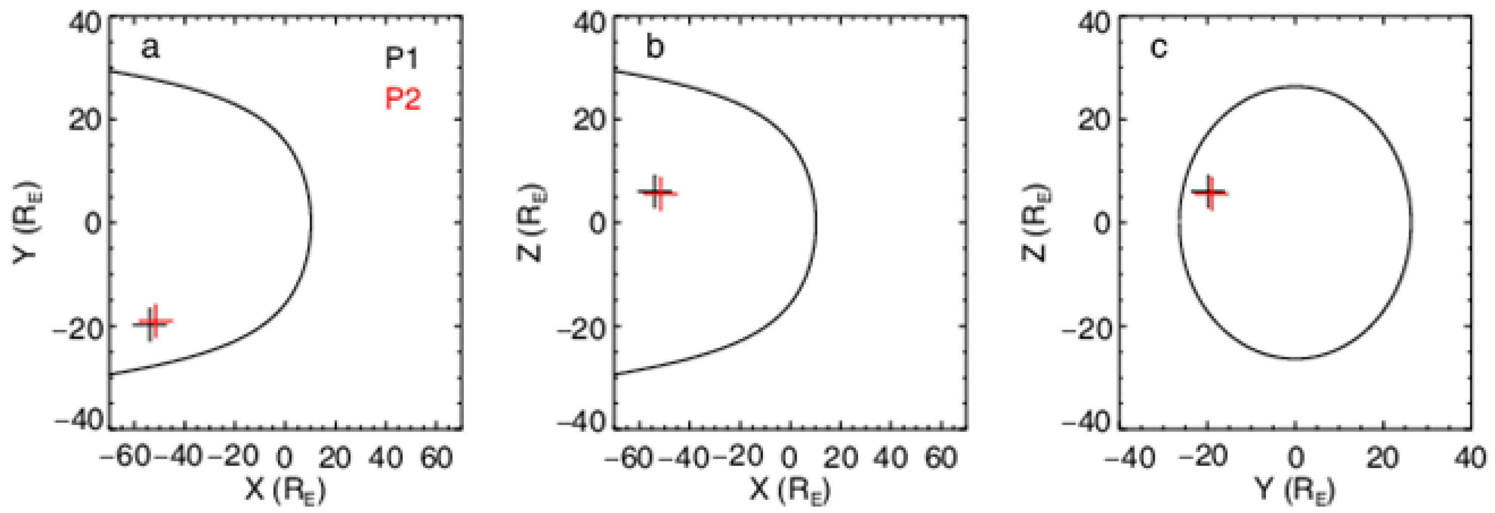
On 18 September 2016, P1 and P2 were in the magnetotail near the lunar orbit and crossed the magnetopause several times, and they observed quasi-periodic fluctuations of magnetic field, plasma density, and temperature. The locations of P1 and P2 in GSM coordinates are shown in
Figure 1. The curved lines are the magnetopause obtained from Shue et al. [
27] model; the upstream solar-wind dynamic pressure and IMF
Bz are −2.87 nP and 1.65 nT, respectively.
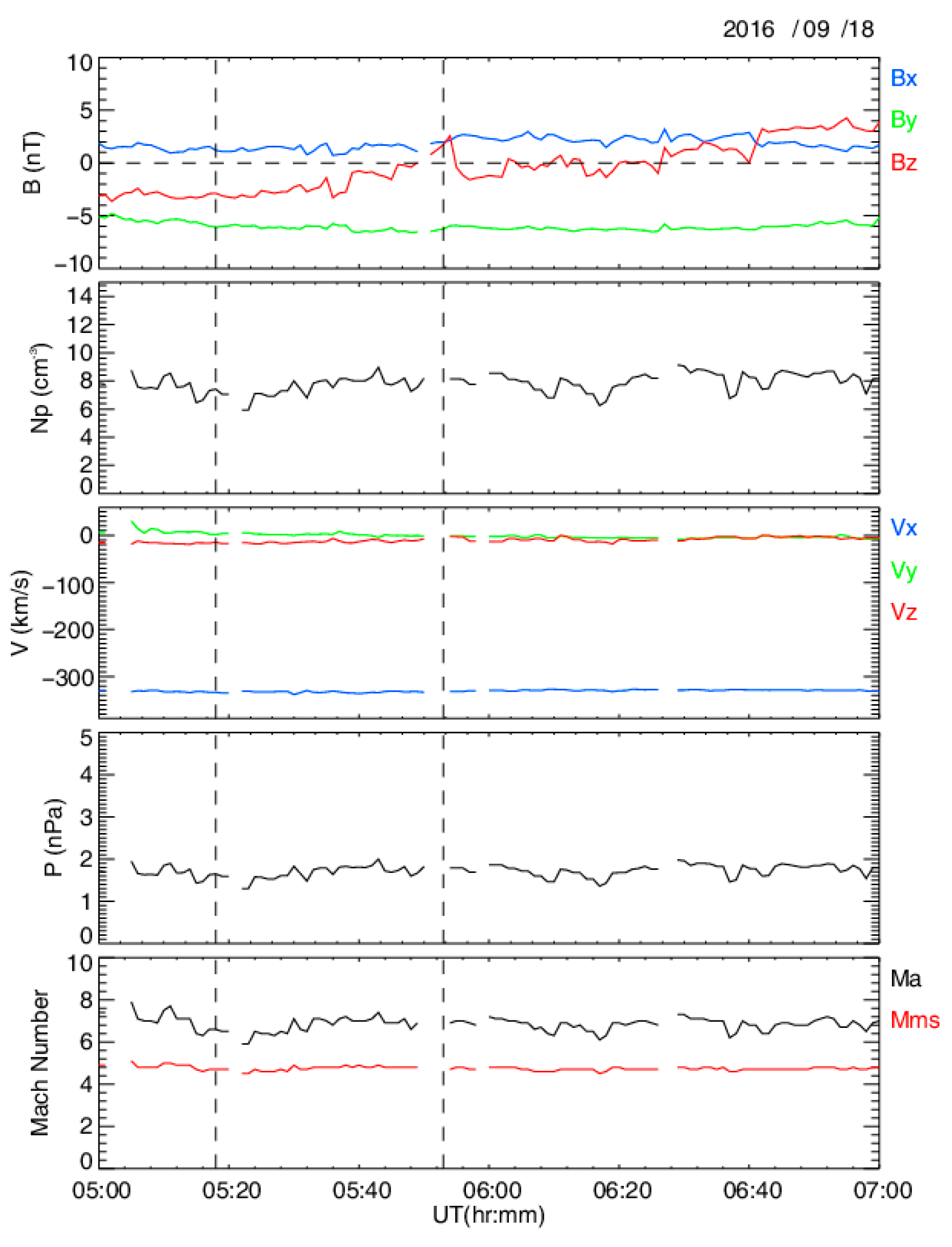
The upstream solar-wind conditions of this event are obtained from the OMNI database (
Figure 2). The delay time is obtained by the solar-wind velocity and the distance between the observed event and the position of the nose of the bow shock, which is about 22 min for this event. From
Figure 2 we can see that the IMF
Bz is southward during the period of KH waves, except for a few minutes.
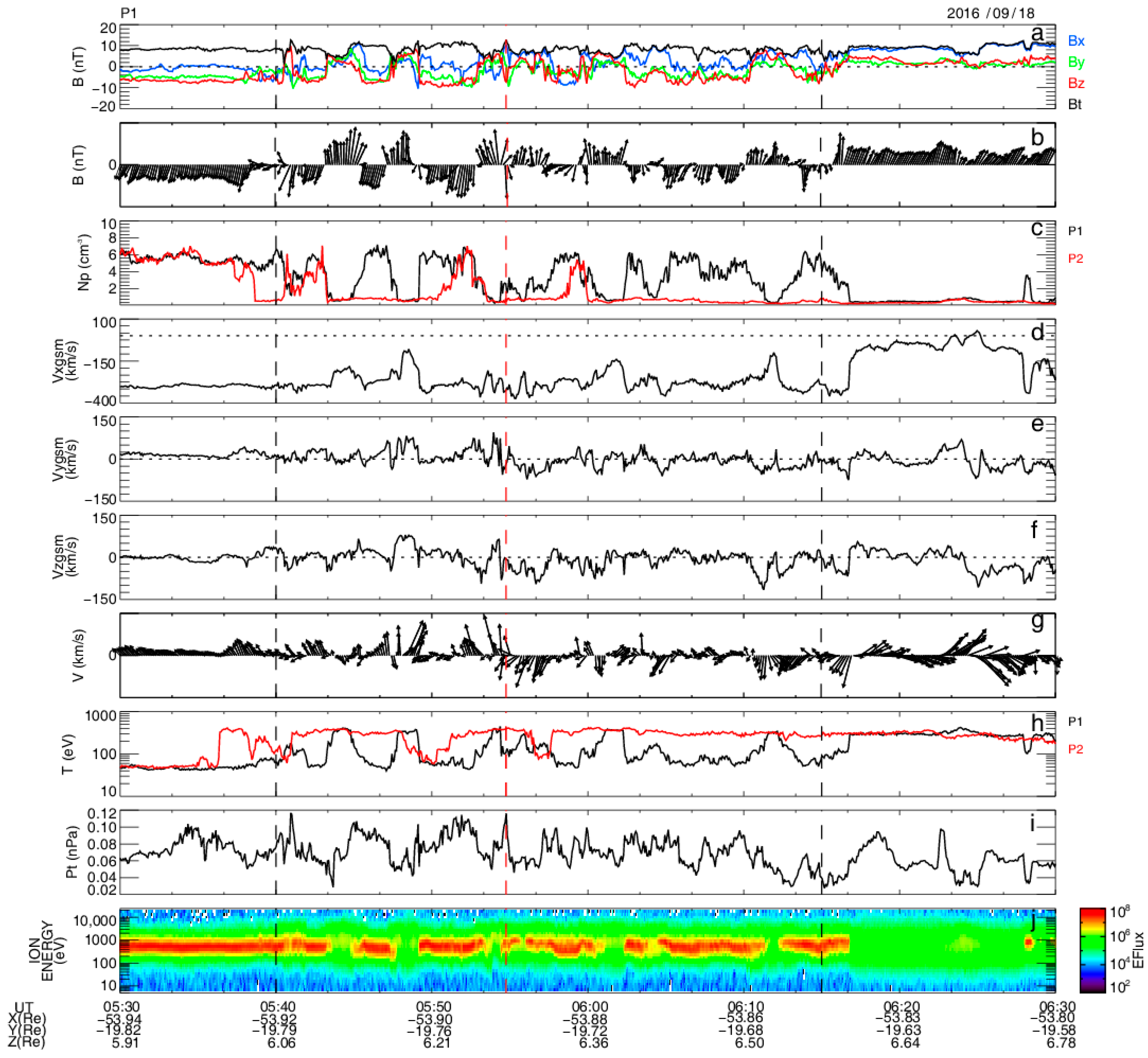
Figure 3 shows the overview observations of P1 from 05:30 UT to 06:30 UT. At 05:30 UT, P1 was located in the magnetosheath, which is characterized by dense (~6 cm
−3) and cold (<100 eV) plasma. Then, P1 entered the magnetospheric boundary layer accompanied by a decrease in density and an increase in temperature. From
Figure 3b,g, we can see vortical magnetic-field perturbations and vortical velocity perturbations, which indicate the existence of KH waves during the interval. During this period, there are about nine identifiable wave periods observed by P1, and the perturbations in upstream solar-wind dynamic pressure and IMF
Bz are less than 0.7 nPa and 6 nT, which can be regarded as quasi-steady conditions, as shown in
Figure 2. We further checked whether such smaller fluctuations in dynamic pressure and
Bz can cause the motion of magnetopause. At 05:41:50 UT, P1 and P2 were all located in the magnetosheath, and at 05:42:20 UT and 05:43:30 UT, P2 and P1 entered the magnetosphere subsequently. The delay time is about 22 min for this event. Thus, we calculated the shape and position of the magnetopause using Shue et al. [
27]’s model using the upstream conditions at 05:42:00 UT and 05:44:00 UT. The flare angle of magnetopause moves a little (from 0.622 to 0.618) which is much smaller than the distance between P1 and P2, as shown in
Figure 1. Thus, we believe that the multicrossings of the magnetopause are caused by KH waves rather than changes in upstream conditions. In addition, the P2 was located closer to the Earth than P1, but P1 observed lower plasma density than P2 when the time delay was considered (
Figure 3c). The delay time was estimated from the time that two spacecraft passed similar density profiles [
15], and the delay time was 68 s for this event. Although there exists some difference in the two density profiles, the delay time for this event still gives the best correlations between the two spacecraft. The difference may be caused by the variation of the waveform across the boundary layer. We also calculated the propagation velocities using the propagation time. P1 and P2 were located at (−53.92, −19.79, 6.06) R
E and (−51.53, −19.04, 5.52) R
E, which were separated by around 2.39 R
E, 0.75 R
E, and 0.54 R
E from each other in X direction, Y direction, and Z direction, respectively. Thus, the propagation velocity of the first KH-wave structure is around (−223, 70, 51) km/s. The total separation and velocity are 2.56 R
E and 240 km/s.
The unstable condition of KH instability under the assumption of plasma incompressibility and no boundary thickness is shown in Equation (1).
where
is the shear velocity between magnetosphere and magnetosheath,
and
are the magnetic field and mass density, and the subscripts “1” and “2” represent the magnetosphere and magnetosheath sides, respectively. The
k is wave vector, and we regard the
L direction in LMN as the
k direction for this case. We obtain
N direction from the Minimum Faraday Residue (MFR) analysis in the magnetic field [
28] and the electric field derived from ion velocity (
). Then, we calculate the
M direction from cross-product of the
N direction and the maximum variance direction from MVAV (minimum variance analysis velocity) [
29], and the
L direction is determined as the cross-product of the
M and
N direction. For this event, the density, velocity, and magnetic field in magnetosheath and magnetosphere were obtained from the 5 min averaged value of 05:25 UT–05:30 UT and 06:18 UT–06:23 UT, respectively. The density in magnetosphere and magnetosheath were respectively about 0.7 cm
–3 and 8.5 cm
–3. The magnetic field
B1 = (8.58, 1.85, 2.49) nT and
B2 = (
1.07,
4.32,
6.46) nT. The
V0 and
k are (247.46, 20.86, 12.61) km/s and (0.73,
0.45, 0.5), respectively. The threshold of the shear velocity is 240 km/s which is smaller than
V0. This indicates that the KHI is satisfied for this event.
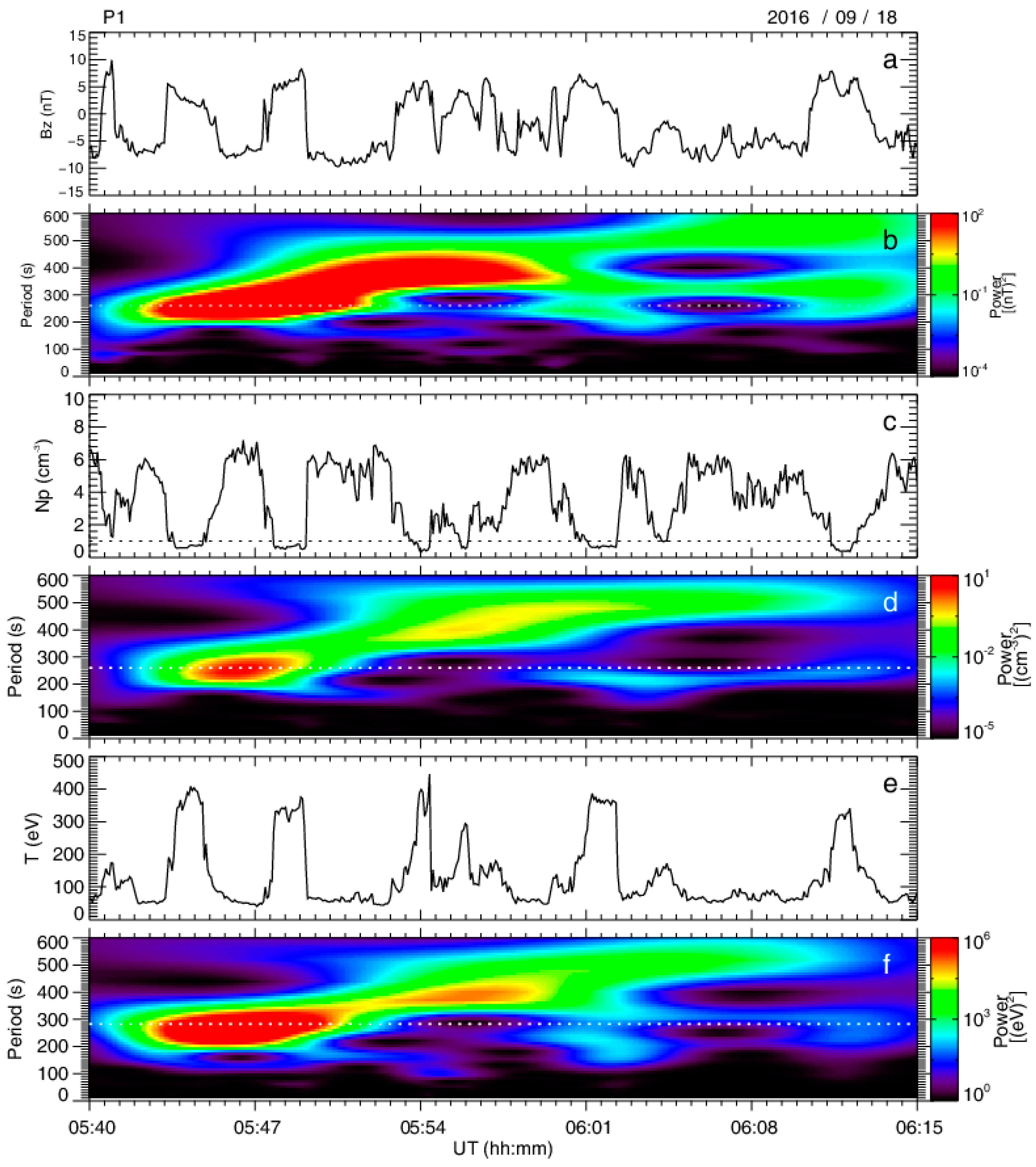
The phase velocity, dominant period, and wavelength are the intrinsic characters of KH waves. The wavelet-analysis method is used to estimate the dominant period of this event. The wavelet-spectrum analysis of ion density,
Bz, and ion temperature during 05:40 UT to 06:15 UT is shown in
Figure 4. The wavelet analysis of the density and temperature shows two different peaks during 05:40 UT to 06:15 UT. Before 05:53 UT, we can see the strong peaks at 260 s and 283 s for the density and temperature, respectively, which are also close to the intuitive counting of the density and temperature fluctuations, 233 s. After 05:59 UT, the density and ion temperature show the peak period at 477 s and 479 s. The change in the wave periods may correspond to the change in the spacecraft locations relative to the wave center [
19]. In
Figure 4, in the earlier time, longer intervals of magnetosphere-like low-density and high-temperature plasmas can be seen, while in the later time, we can see longer intervals of magnetosheath-like high-density and low-temperature plasmas, which may indicate that the spacecraft moved from the magnetospheric to magnetosheath sides of the waves during the whole interval in
Figure 4. In addition, a very long interval of the high-density and low-temperature plasmas can be seen after 06:00. This may correspond to the spacecraft that moved too far away from the wave center—that is, that the spacecraft just missed the wave structures in the later time in
Figure 4, and the true wave period was seen in the earlier time. In addition,
Bz shows a strong peak at 260 s before 05:53 UT. Therefore, we adopt the mean peak period of
Bz, temperature, and density, 268 s, before 05:53 UT as the dominant period.
There are two methods to estimate the phase velocity of the KH waves. The phase velocity is between the average velocity
and center-of-mass velocity (
) with the shear layer with finite thickness, where the “1” and “2” represent the magnetosphere and magnetosheath, respectively. For the KH waves on the zero-thickness shear layer, the phase velocity is equal to the center-of-mass velocity (
). Lin et al. [
30] indicate that the velocity of the vortex center-of-mass can represent the phase velocity by comparing the center-of-mass velocity with the velocity estimated by the four-spacecraft timing analysis [
31]. Here we use the center-of-mass,
, to represent the phase velocity, as previous works did [
14,
30]. The phase velocity, in this case, is 287 km/s estimated from the interval 05:40 UT–06:15 UT, which is close to the propagation velocity of the first KH-wave structure, 240 km/s. This also indicates the observed waves are KH waves. The wavelength for this event can be estimated as 268 s × 287 km/s = 12.07 R
E.
3. Discussion
For the KH waves under the northward IMF, Hasegawa et al. [
10] proposed a criterion to distinguish it when observed by a single spacecraft. There are three items for identifying the KH wave: (1) The quasi-periodic fluctuations with the period in the magnetic field and plasma; (2) During the observation of KH waves, the upstream solarwind conditions and even the magnetosheath conditions are quasi-steady, and there is no perturbation with a similar period. (3) There exists a sufficient number of data points with low density (lower than the half of the density of magnetosheath plasma) and high speed (higher than the speed of magnetosheath plasma). Both Hwang [
15] and Blasl [
18] showed that this analysis of low-density and faster-than-sheath plasma can work even for the southward-IMF cases. We checked the velocity and density distribution of this event and found that there also exists low-density and faster-than-sheath plasma, as shown in the lower-left part of
Figure 5. This further indicates that the vortex structures are generated near the magnetopause.
A chain of flux-transfer events (FTE) crossing through the spacecraft can produce quasi-periodic structures, which may be similar to the KH waves in the nonlinear stage [
24,
32,
33]. For the FTE and KH wave,
BN both have bipolar perturbations. However, the maximum value of the magnetic field strength often occurs at the edge of the vortex for the KH wave, and occurs at the core of FTE. The bipolar perturbations are also continuous for the KH wave. Another difference in the FTE and KH wave is that there exists a maximum value in total pressure at the center for FTE, and the maximum value of total pressure often occurs at the edge of the KH wave and the minimum value of total pressure often occurs at the center of the KH vortex. The characteristics of
VN are also different; the
VN of KH wave is quasi-steady and the perturbation of
VN for FTE is relatively large and typically has a bipolar structure. In this event,
BN has bipolar perturbations, and the peak value of magnetic field strength and pressure occur at the edge of the vortex for most of the time, as shown by the black dashed vertical lines in
Figure 6. The perturbations of
VN are small, smaller than 150 km/s, and there is no bipolar structure in
VN. Therefore, we believe this is a KH-wave event. Note, however, that a total pressure peak at around 05:55 UT is probably not of a KH wave, but of an FTE event with bipolar
By (
Figure 2).
It is also indicated that there are plasmas with low density and high speed in KH waves, and the plasmas with these characteristics cannot be found in the FTE. However, as mentioned above, the low-density and high-speed flow can also be caused by reconnection for the event under southward IMF. Therefore, here we do not use this criterion to distinguish FTE and KH waves. The period of the KH wave is in the range of 1–4 min and the period of FTE is typically longer for the period of the KH wave, which has the maximum value at 4 min. For this event, the dominant period is 268 s, which coincides with this characteristic. Muria [
34] used the observations within 30 R
E to study the spatial distribution of the period of the KH waves, and they showed that with the increasing distance from the subsolar point of magnetopause, the period increases due to the vortex merging when the KH waves flow to the tail. Using the linear relationship from Muria [
34], T =
, where the
is the distance from the subsolar point of magnetopause, we can obtain that the period is 734 s using the typical subsolar point of magnetopause, (10, 0, 0) R
E. This result is larger than our result obtained from wavelet analysis, 272 s. This is probably because Muria [
34] only used the observations within 30 R
E to fit this relationship.
The KH waves under the southward IMF at the flank magnetopause have been reported by Hwang et al. [
15], Yan et al. [
16], Nakamura et al. [
19], and Basl et al. [
20]. Hwang et al. [
15], indicated that the KH waves tend to be irregular and intermittent under the southward IMF when compared to the KH waves under the northward IMF. Our observations also have irregular and intermittent characteristics similar to Hwang et al. [
15]. Yan et al. [
16] reported the KH vortices at the duskside of the magnetopause under the southward IMF, and the period and propagation speed were estimated as 4 min and 292 km/s, respectively. The wavelength is about 11 R
E, which is smaller than our result of 12.25 R
E. In addition, the wavelength of most KH waves under the northward IMF at near-Earth magnetopause is less than 10 R
E as shown in
Figure 7 of Lin et al. [
30], which is also smaller than our result. The results indicate that the wavelength increases as the distance from the subsolar point increases. The KH waves at the lunar distance under northward IMF were reported by Ling et al. [
14], and the wavelength of this event is 11.1 R
E, which is also similar with our results.
We further investigated the normal direction of the magnetopause using minimum-variance analysis of the magnetic field.
Figure 7a–d presents the tangential planes of magnetopause estimated from the normal direction in the XY plane at 05:43:10 UT, 05:45:30 UT, 05:47:40 UT, and 05:49:00 UT. The ratio of the second to third eigenvalues of MVA are 9.09, 13.71, 9900, and 21.99, which indicate that the MVA is reliable for these cases.
Figure 7e shows the schematic of the KH vortices estimated by the tangential planes. From
Figure 7 we can see that the magnetopause was deformed by KH waves.


