Connections between the Shadow Radius and the Quasinormal Modes of Kerr-Sen Black Hole

Abstract

The correspondence between the shadow radius and the real part of the quasinormal modes (QNMs) of a Kerr–Sen black hole is studied. By using the equation of the shadow radius of Kerr–Sen black hole and the angular separation constant of the QNMs, the expression of QNMs related to shadow radius is established in the eikonal limit. We found that, our formula can reduce to the previous result of Kerr black hole when Kerr-Sen parameter b sets to zero.

1. Introduction

In 2019 the Event Horizon Telescope (EHT) Cooperation released the first black hole shadow image of M87* [1,2,3,4,5,6], and later in 2022 the EHT Cooperation further released its image for SgrA* [7]. In addition to the influence of the observer’s angle, the shadow also contains information such as the mass and the rotating parameters of the black holes. Moreover, the black hole shadow can serve as a tool to test the theory of gravity and thus receives increasing attention. On the other hand, the first gravitational wave event was observed by the LIGO Scientific Collaboration in 2015 [8]. This is the first time that gravitational waves have been observed in history, which cast a great influence and promotion on science. The characteristic modes of an exponentially decaying ringdown phase of the gravitational waves are described by quasinormal modes (QNMs), and can be decomposed as ${\omega }_{QNM}={\omega }_R-i{\omega }_I$ where the real part represents the frequency of the wave, and the imaginary part represents the damping.

Though the QNMs and the black hole shadow seem irrelevant to each other at the first glance, they in fact have a deep connection. In 2009, by using the WKB approximation method [9,10,11] to calculate of QNMs, V. Cardoso et al. [12] established the first concrete correspondence between QNMs and the black hole shadows for a static spherically symmetric asymptotically flat black hole in the eikonal limit, $\ell \gg 1$ (ℓ is the integer angular number). Their results [12] show the real part of the QNMs corresponding to the frequency of the circular null geodesic, while the imaginary part corresponds to the Lyapunov constant that determines the scale of orbital instability. However, although such a correspondence formula looks very elegant, it was soon to be found not applicable to some modified gravity theories [13]. Another question is how to extend the correspondence to the rotational black hole case, since most astrophysical real black holes process rotation. More recently, the relation between the QNMs and black hole shadow for rotating black hole are proposed by H. Yang et al. [14] and K. Jusufi [15,16] respectively. Their results coincide at the large ℓ limit. For examples, they study the Kerr, Kerr–Newman, as well as the five-dimensional Myers–Perry black holes [14,15,16,17]. However, generalizing this correspondence to the more general case to test its domain of validation is still crucial, especially for the black hole in modified gravity theory.

The Kerr–Sen (KS) black hole [18] is an exact black hole solution in the low-energy effective field theory of the heterotic string theory. It represents a charged and rotating black hole. Many aspects of KS black holes have been investigated in the past three decades [19,20,21,22,23,24]. Particularly, the shadow of the KS black hole has been calculated in Refs. [25,26,27]. Since in the modified gravity theories, the quasi-normal modes and the black hole shadow will both be changed, the KS black hole serves as an ideal extension to further verify the correspondence between the shadow of the rotational black hole and its QNMs. For the motivations given above, we are going to study the connection between the shadow radius and the QNMs in the KS spacetime.

This article is organized as follows. Section 1 is an introduction. Then we give the basic equations of motion for KS black hole in Section 2. We further calculate the shadow radius by using the unstable photon orbit in Section 3. In Section 4, after analyzing the perturbations of the massless scalar field and discussing the angular separation constant, we establish the relation between the QNMs and the shadow radius of the KS black hole. The conclusion is given in Section 5. Throughout this paper, we adopt the geometric units such that $G=c=\hslash =1$.

2. Basic Equations

The author in [18] constructs an exact classical black hole solution in the low-energy effective field theory of the heterotic string theory. Note that the low-energy effective action of heterotic string theory in four dimensions can be expressed as

$$\begin{array}{c}\hfill S=-\int d^{4}x\sqrt{-\tilde{g}}{e}^{-\mathrm{\Phi }}\left(-R+\frac{1}{12}{H}_{\mu \nu \rho }{H}^{\mu \nu \rho }-g^{\mu \nu }{\partial }_{\mu }\mathrm{\Phi }{\partial }_{\nu }\mathrm{\Phi }+\frac{1}{8}{F}_{\mu \nu }{F}^{\mu \nu }\right),\end{array}$$

(1)

where $\tilde{g}$ is a determinant of metric tensor ${\tilde{g}}_{\mu \nu }$, R is the Ricci scalar, $\mathrm{\Phi }$ is the dilaton field, $F_{\mu \nu }={\partial }_{\mu }{A}_{\nu }-{\partial }_{\nu }{A}_{\mu }$ corresponding to the Maxwell field. Moreover, $H_{\mu \nu \rho }$ is the third-rank field defined as

$$\begin{array}{c}\hfill H_{\mu \nu \kappa }={\partial }_{\kappa }{B}_{\mu \nu }+{\partial }_{\mu }{B}_{\nu \kappa }+{\partial }_{\nu }{B}_{\kappa \mu }-\frac{1}{4}\left(A_{\kappa }{F}_{\mu \nu }+A_{\mu }{F}_{\nu \kappa }+A_{\nu }{F}_{\kappa \mu }\right),\end{array}$$

(2)

with $B_{\mu \nu }$ being a second-rank antisymmetric tensor field.

By rescaling the metric $g_{\mu \nu }=e^{-\mathrm{\Phi }}{\tilde{g}}_{\mu \nu }$, such a theory admits a four dimensional black hole solution in Einstein frame usually referred to as KS black hole [18,28,29]. Since in an Einstein frame, the gravity and matter fields (including the dilaton field and tensor field) are minimally coupled to each other, and therefore many familiar properties about gravity are still valid. For instance, in the Einstein frame, we observe that the black hole entropy product is universal [28]. This solution is characterized by its mass M, charge Q and rotating parameter a. In Boyer–Lindquist coordinates $(t,r,\theta ,\phi )$, the metric of KS black hole reads [18,28,29]

$$\begin{array}{ccc}\hfill d{s}^2& =& \hfill -\left(1-\frac{2Mr}{{\rho }^2}\right)d{t}^2+{\rho }^2\left(\frac{d{r}^2}{{\Delta }_{KS}}+d{\theta }^2\right)-\frac{4Mra}{{\rho }^2}{sin}^2\theta dtd\phi +\hfill \\ & & \hfill \left(r(r+2b)+a^2+\frac{2Mr{a}^2{sin}^2\theta }{{\rho }^2}\right){sin}^2\theta d{\phi }^2,\hfill \end{array}$$

(3)

where

$$\begin{array}{c}\hfill {\Delta }_{KS}=r^2-2Mr+2br+a^2,{\rho }^2=r^2+2br+a^2{cos}^2\theta .\end{array}$$

(4)

Here the relation between the parameter b and charge Q is $b=Q^2/2M$. The horizon of the KS black hole is determined by ${\Delta }_{KS}=0$, and therefore is given by $r_{\pm }=M-b\pm \sqrt{{(M-b)}^2-a^2}$.

The geodesic Hamilton–Jacobi equation of a KS black hole reads [30]

$$\begin{array}{c}\hfill \frac{\partial S}{\partial \sigma }=-\frac{1}{2}{g}^{\mu \nu }\frac{\partial S}{\partial x^{\mu }}\frac{\partial S}{\partial x^{\nu }},\end{array}$$

(5)

where S, $\sigma$ is the principal function and an affine parameter, respectively. For the null geodesics, the corresponding principal function S reads [30]

$$\begin{array}{c}\hfill S(t,r,\theta ,\phi )=-Et+S_r\left(r\right)+S_{\theta }\left(\theta \right)+L_z\phi ,\end{array}$$

(6)

Combining Equation (6) with Equation (5), we obtain two separated parts of the Hamilton–Jacobi equation [30,31]

$$\begin{array}{c}\hfill S_r\left(r\right)=\pm \int \frac{R\left(r\right)}{{\Delta }_{KS}}dr,S_{\theta }\left(\theta \right)=\pm \int \sqrt{\mathrm{\Theta }\left(\theta \right)}d\theta ,\end{array}$$

(7)

where

$$\begin{array}{c}\hfill R\left(r\right)={(a{L}_z-E(r(r+2b)+a^2))}^2-{\Delta }_{KS}({(L_z-aE)}^2+\mathcal{D}),\end{array}$$

(8)

$$\begin{array}{c}\hfill \mathrm{\Theta }\left(\theta \right)=\mathcal{D}-{cos}^2\theta \left(\frac{L_z^2}{{sin}^2\theta }-a^2{E}^2\right).\end{array}$$

(9)

The constants E and $L_z$ are the energy and the angular momentum of the photon, respectively, and $\mathcal{D}$ is commonly referred to as the Carter separation constant [30,32,33].

Considering the Hamilton–Jacobi Equation (5), the equations of motion of particles in the KS spacetime are determined by the following four first order linear differential equations

$$\begin{array}{ccc}\hfill {\rho }^2\dot{t}& =& \hfill \frac{E{(r(r+2b)+a^2)}^2-2Mra{L}_z}{{\Delta }_{KS}}-a^2{E}^2{sin}^2\theta ,\hfill \end{array}$$

(10)

$$\begin{array}{ccc}\hfill {\rho }^2\dot{\phi }& =& \hfill -aE+\frac{L_z}{{sin}^2\theta }+\frac{a}{{\Delta }_{KS}}(r(r+2b)+a^{2}E-a{L}_z),\hfill \end{array}$$

(11)

$$\begin{array}{ccc}\hfill {\rho }^2\dot{\theta }& =& \hfill \pm \sqrt{\mathrm{\Theta }\left(\theta \right)},\hfill \end{array}$$

(12)

$$\begin{array}{ccc}\hfill {\rho }^2\dot{r}& =& \hfill \pm \sqrt{R\left(r\right)},\hfill \end{array}$$

(13)

3. Shadow Radius of the Kerr–Sen Black Hole

The size and shape of the shadow of a black hole are determined by the unstable circular photon orbit. For the observer at infinity, the observed shape is also affected by the inclination angle ${\theta }_0$ of the observer. Consider the circular unstable photon orbit in the equatorial plane ($\theta =\pi /2$). The appropriate Lagrangian is

$$\begin{array}{c}\hfill \mathcal{L}=\frac{1}{2}{g}_{\mu \nu }\dot{x^{\mu }}\dot{x^{\nu }}.\end{array}$$

(14)

Since the KS spacetime is stationary and axially symmetric, from the conserved quantities of the test particle, we can conclude that

$$\begin{array}{ccc}\hfill p_t=\frac{\partial \mathcal{L}}{\partial \dot{t}}& =& \hfill g_{tt}\dot{t}+g_{t\phi }\dot{\phi }=E,\hfill \end{array}$$

(15)

$$\begin{array}{ccc}\hfill p_{\phi }=\frac{\partial \mathcal{L}}{\partial \dot{\phi }}& =& \hfill g_{t\phi }\dot{t}+g_{\phi \phi }\dot{\phi }=-L_z,\hfill \end{array}$$

(16)

$$\begin{array}{ccc}\hfill p_r=\frac{\partial \mathcal{L}}{\partial \dot{r}}& =& \hfill g_{rr}\dot{r}.\hfill \end{array}$$

(17)

For the null geodesics in the equatorial plane, the corresponding Hamiltonian is

$$\begin{array}{c}\hfill H=p_t\dot{t}+p_{\phi }\dot{\phi }+p_r\dot{r}-\mathcal{L}=0.\end{array}$$

(18)

Here we will introduce $V_{eff}$ as the effective potential of the photon [12] which is defined as

$$\begin{array}{c}\hfill V_{eff}={\dot{r}}^2.\end{array}$$

(19)

Then combining the above definition with Equation (18), we can obtain

$$\begin{array}{c}\hfill V_{eff}=-\frac{g_{tt}{\dot{t}}^2+2g_{t\phi }\dot{t}\dot{\phi }+g_{\phi \phi }{\dot{\phi }}^2}{g_{rr}}.\end{array}$$

(20)

For a circular photon orbit, it is required that [34]

$$\begin{array}{c}\hfill V_{eff}=0,V_{eff}^{{}^{\prime }}=0.\end{array}$$

(21)

By simplifying Equation (21) we can get the following two equations:

$$\begin{array}{c}\hfill \left(a^2(2b+2M+r)+r{(2b+r)}^2\right)E^2-4a{L}_{z}ME-L_z^2(2b-2M+r)=0,\end{array}$$

(22)

and

$$\begin{array}{c}\hfill -a^2{E}^{2}M+2aE{L}_{z}M+4b^3{E}^2+8b^2{E}^{2}r+5b{E}^2{r}^2+E^2{r}^3-L_z^{2}M=0.\end{array}$$

(23)

Note that the black hole shadow radius $R_s$ can be expressed as $R_s=L_z/E$ [15]. Then Equation (23) is equivalent equals to

$$\begin{array}{c}\hfill {(R_s-a)}^{2}M-(8b^{2}r+5b{r}^2+r^3+4b^3)=0,\end{array}$$

(24)

which implies that

$$\begin{array}{c}\hfill R_s^{\pm }=a\pm \sqrt{\frac{4b^3+8b^2{r}_0^{\pm }+5b{\left(r_0^{\pm }\right)}^2+{\left(r_0^{\pm }\right)}^3}{M}}.\end{array}$$

(25)

Here $r_0^{\pm }$ are the solutions of Equation (22) by substituting Equation (25) into Equation (22). When viewed from the equatorial plane (${\theta }_0=\pi /2$). The typical shadow radius for a rotating black hole can be defined as [35,36]

$$\begin{array}{c}\hfill {\overline{R}}_s=\frac{1}{2}(x\left(r_0^{+}\right)-x\left(r_0^{-}\right)),\end{array}$$

(26)

here $x\left(r_0^{\pm }\right)$ denoting the unstable photon orbits [15,35]. In such a situation the definition in Equation (26) equals to

$$\begin{array}{c}\hfill {\overline{R}}_s=\frac{1}{2}(R_s^{+}{|}_{r_0^{+}}-R_s^{-}{|}_{r_0^{-}}).\end{array}$$

(27)

Then the typical shadow radius for KS black hole reads

$$\begin{array}{c}\hfill {\overline{R}}_s=\frac{1}{2}\left(\sqrt{\frac{4b^3+8b^2{r}_0^{+}+5b{\left(r_0^{+}\right)}^2+{\left(r_0^{+}\right)}^3}{M}}+\sqrt{\frac{4b^3+8b^2{r}_0^{-}+5b{\left(r_0^{-}\right)}^2+{\left(r_0^{-}\right)}^3}{M}}\right).\end{array}$$

(28)

It is a function of the black hole mass M, the rotating and the charge parameter a, b respectively. In this paper, we have set the black hole mass $M=1$. From Figure 1 it can be concluded that the shadow radius decreases with the increases of the charge parameter b, and for the same value of b, the larger of the rotating parameter a corresponds to the smaller radius.

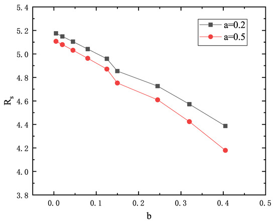
Figure 1. The shadow radius of KS black hole for different values of b when the rotating parameter chosen as a = 0.2 or a = 0.5.

4. QNMs of the Kerr–Sen Black Hole

4.1. Perturbation of the Scalar Field

Considering a massless scalar field H in the KS spacetime, it satisfied the Klein–Gorden equation

$$\begin{array}{c}\hfill \frac{1}{\sqrt{-g}}{\partial }_{\alpha }\left(g^{\alpha \beta }\sqrt{-g}{\partial }_{\beta }H\right)=0.\end{array}$$

(29)

Teukolsky’s work [37] shows that all the scalar fields which satisfied ${\nabla }^{2}H=0$ are separable in Boyer–Lindquist coordinates, such that from Equation (29) we can get the master perturbation equation

$$\begin{array}{c}\left(a^2{sin}^2\theta -\frac{{(r^2+2br+a^2)}^2}{{\Delta }_{KS}}\right)\frac{{\partial }^{2}H}{\partial t^2}-\frac{4Mra}{{\Delta }_{KS}}\frac{{\partial }^{2}H}{\partial t\partial \phi }+\left(\frac{1}{sin\theta }-\frac{a^2}{{\Delta }_{KS}}\right)\frac{{\partial }^{2}H}{\partial {\phi }^2}+\hfill \\ \frac{\partial }{\partial r}\left({\Delta }_{KS}\frac{\partial H}{\partial r}\right)+\frac{1}{sin\theta }\frac{\partial }{\partial \theta }\left(sin\theta \frac{\partial H}{\partial \theta }\right)=0.\hfill \end{array}$$

(30)

For the scalar field $H(t,r,\theta ,\phi )$ in the KS spacetime, we can decompose it as [38,39]

$$\begin{array}{c}\hfill H=e^{-i\omega t}{e}^{im\phi }R\left(r\right)S\left(\theta \right).\end{array}$$

(31)

By substituting Equation (31) into Equation (30) we can get two separable equations for $S\left(\theta \right)$ and $R\left(r\right)$:

$$\begin{array}{c}\frac{1}{sin\theta }\frac{d}{d\theta }\left(sin\theta \frac{dS\left(\theta \right)}{d\theta }\right)+\left(a^2{\omega }^2{cos}^2\theta -\frac{m^2}{{sin}^2\theta }+A_{\ell m}\right)S\left(\theta \right)=0,\hfill \\ \frac{d}{dr}\left({\Delta }_{KS}\frac{dR\left(r\right)}{dr}\right)+\left(\frac{{(\omega (r^2+2br+a^2)-am)}^2}{{\Delta }_{KS}}+2am\omega -a^2{\omega }^2-A_{\ell m}\right)\hfill \end{array}$$

(32)

$$\begin{array}{c}R\left(r\right)=0,\hfill \end{array}$$

(33)

where m and $A_{\ell m}$ are the azimuthal quantum number and the angle eigenvalue, respectively. $A_{\ell m}$ is a function of $\omega$. When the parameter a and b take to zero (the Schwarzschild limit), the angle eigenvalue takes a simple form as $A_{\ell m}=\ell (\ell +1)$. In general, the expression of $A_{\ell m}$ is quite complicated and we can usually separate $A_{\ell m}$ into real and imaginary parts [40]

$$\begin{array}{c}\hfill A_{\ell m}=A_{\ell m}^R-i{A}_{\ell m}^I.\end{array}$$

(34)

For Equation (32) it should satisfy the Bohr–Sommerfeld quantization condition [40]

$$\begin{array}{c}\hfill {\int }_{{\theta }_{-}}^{{\theta }_{+}}\sqrt{a^2{\omega }_R^2{cos}^2\theta -\frac{m^2}{{sin}^2\theta }+A_{\ell m}^R}d\theta =(L-\mid m\mid )\pi .\end{array}$$

(35)

Here we have set $L=\ell +1/2$ [40]. ${\theta }_{\pm }$ are the turning point and the zero point of the potential. For the angular equation Equation (32), motivated by the WKB analysis, defining $dx=d\theta /sin\theta$, $x=log(tan\frac{\theta }{2})$, Equation (32) can be rewritten as

$$\begin{array}{c}\hfill \frac{d^{2}S\left(\theta \right)}{d{x}^2}+(a^2{\omega }_R^2{cos}^2\theta {sin}^2\theta -m^2+A_{\ell m}^R{sin}^2\theta )S\left(\theta \right)=0.\end{array}$$

(36)

Equation (32) has two regular singular points, $cos\theta =+1$ and $cos\theta =-1$. The boundary condition for Equation (32) is that $S_{\theta }$ being finite at the singular points. Similar to E. W. Leaver [41], we can write a solution to Equation (32) as [41]

$$\begin{array}{c}\hfill S_{\theta }=e^{a\omega cos\theta }{(1+cos\theta )}^{\frac{\left|m\right|}{2}}{(1-cos\theta )}^{\frac{\left|m\right|}{2}}\sum _{n=0}^{\infty }{a}_n{(1+cos\theta )}^n.\end{array}$$

(37)

By substituting Equation (37) into Equation (32), we can get a three-term recurrence relation:

$$\begin{array}{ccc}& & \hfill {\alpha }_0{a}_1+{\beta }_0{a}_0=0.\hfill \end{array}$$

(38)

$$\begin{array}{ccc}& & \hfill {\alpha }_n{a}_{n+1}+{\beta }_n{a}_n+{\gamma }_n{a}_{n-1}=0.n=1,2...\hfill \end{array}$$

(39)

For given values of a and m, ${\omega }_R$ and $A_{\ell m}$ can be found by solving the continued fraction equation. Particularly, in the eikonal limit with $\ell \gg 1$, we can take $a{\omega }_R$ as a small value. Then the separation constant $A_{\ell m}^R$ can be expanded as a Taylor series [41]. That is:

$$\begin{array}{c}\hfill A_{\ell m}^R=\sum _{p=0}^{\infty }{f}_p{\left(a{\omega }_R\right)}^p\approx f_0+f_2{\left(a{\omega }_R\right)}^2+O{\left(a{\omega }_R\right)}^4\approx L^2+\frac{1}{2}(\frac{m^2}{L^2}-1)a^2{\omega }_R^2.\end{array}$$

(40)

4.2. Connections between the QNMs and Shadow Radius

By identifying the massless scalar field H with the leading order of the principal function (6), we can rewrite it as

$$\begin{array}{c}\hfill H=e^{iS}=e^{-iEt}{e}^{i{L}_z\varphi }{e}^{i{S}_{\theta }}{e}^{i{S}_r}.\end{array}$$

(41)

After comparing Equation (31) with Equation (41), it is not difficult to conclude that

$$\begin{array}{c}\hfill E={\omega }_R,L_z=m.\end{array}$$

(42)

Moreover, when considering Equations (7), (32) and (36), and using the WKB method used in Ref. [40], we can further make the identification that

$$\begin{array}{c}\hfill \mathcal{D}=A_{\ell m}^R-m^2.\end{array}$$

(43)

For typical QNMs, it can be expressed as [40]

$$\begin{array}{c}\hfill \omega =(\ell +\frac{1}{2}){\Omega }_R\left(\mu \right)-i(n+\frac{1}{2}){\Omega }_I\left(\mu \right),\end{array}$$

(44)

with $\mu \equiv m/(\ell +1/2)$.

For a rotating black hole, we introduce a new angle $\Delta {\phi }_{prec}$ [40,42], it represents the Lense–Thiring-precession frequency of the orbit arises because of the rotation of the black hole [40]. If we define $T_{\theta }$ as a period of motion in the $\theta$ direction, then the corresponding precession frequencies ${\Omega }_{prec}$ is

$$\begin{array}{c}\hfill {\Omega }_{prec}=\frac{\Delta {\phi }_{prec}}{T_{\theta }}.\end{array}$$

(45)

Such that in the rotating black hole the real part of the frequency can be written as [14]

$$\begin{array}{c}\hfill {\Omega }_R={\Omega }_{\theta }\left(\mu \right)+\mu {\Omega }_{prec}\left(\mu \right),\end{array}$$

(46)

with ${\Omega }_{\theta }=2\pi /T_{\theta }$.

Considering a complete cycle of the photon orbit in the $\theta$ direction,

$$\begin{array}{c}\hfill \delta S=L_z\Delta \phi -E{T}_{\theta }+\delta S_{\theta }=0,\end{array}$$

(47)

where $\Delta \phi$ is the azimuth changed after completing a cycle in the direction. It relates to the $\Delta {\phi }_{prec}$ by

$$\begin{array}{c}\hfill \Delta \phi =\Delta {\phi }_{prec}+2\pi \mathrm{sgn}\left(L_z\right),\end{array}$$

(48)

where $\mathrm{sgn}(.)$ evaluates the sign of the argument. For $\delta S_{\theta }$, consider it with Equation (35), we can get the equation that

$$\begin{array}{c}\hfill \delta S_{\theta }=2{\int }_{{\theta }_{-}}^{{\theta }_{+}}\sqrt{\mathrm{\Theta }}d\theta =2{\int }_{{\theta }_{-}}^{{\theta }_{+}}\sqrt{\mathcal{D}-{cos}^2\theta \left(\frac{L^2}{{sin}^2\theta }-a^2{E}^2\right)}d\theta =2\pi (L-L_z).\end{array}$$

(49)

Combining Equations (42), (45)–(49), we found that

$$\begin{array}{c}\hfill \frac{L}{E}=\frac{1}{{\Omega }_{\theta }+\mu {\Omega }_{prec}}=\frac{1}{{\Omega }_R}.\end{array}$$

(50)

By substituting $\mathcal{D}=A_{\ell m}^R-m^2$ into Equation (40), in large ℓ case, there is an equation that

$$\begin{array}{c}\hfill \frac{\sqrt{\mathcal{D}+L_z^2}}{E}\approx R_s.\end{array}$$

(51)

Moreover, combining Equations (40), (43) and (51), we can get that

$$\begin{array}{ccc}\hfill \frac{L^2}{E^2}& =& \hfill \frac{\mathcal{D}+L_z^2}{E^2}+\frac{a^2}{2}\left(1-\frac{m^2}{L^2}\right)\hfill \\ & \approx & \hfill R_s^2+\frac{a^2}{2}\left(1-\frac{m^2}{L^2}\right),\hfill \end{array}$$

(52)

Collecting all the ingredients, for the shadow radius $R_s^{+}$ and $R_s^{-}$, the connection between the real part of the QNMs and the shadow radius is [15]

$$\begin{array}{c}\hfill {\omega }_R=\frac{1}{2}\left({\omega }_{R^{+}}-{\omega }_{R^{-}}\right)\end{array}$$

(53)

with ${\omega }_{R^{\pm }}$ being

$$\begin{array}{c}\hfill {\omega }_{R^{\pm }}=\pm \frac{\ell +\frac{1}{2}}{\sqrt{{\left(R_s^{\pm }\right)}^2+\frac{a^2}{2}(1-{\mu }^2)}}.\end{array}$$

(54)

When take the limit that $\ell \gg 1$, and $m=\pm \ell$ which means $\mu \to 1$. Then the above equation can be reduced to ${\omega }_{R^{\pm }}\approx \frac{\ell }{R_s^{\pm }}$, which agrees with the statement in Ref. [15].

We can get the real part of QNMs of KS black hole by use of correspondence Equation (54). Table 1 shows the QNMs of the black hole obtained by applying geometrical optics approximation to calculate the shadow of the black hole under different values of the parameter b. With the increase of parameter b, the corresponding shadow radius of the black hole decreases gradually and the value of QNMs increases.

Table 1. The shadow radius of KS black hole for different charge parameter b when $a=0.2$.

b	${\mathit{\omega }}_{\mathit{R}}^{+}$	${\mathit{\omega }}_{\mathit{R}}^{-}$	${\overline{\mathit{R}}}_{\mathit{s}}$
0.005	16.81283709	−22.97778200	5.17568286
0.02	16.88189993	−23.12877614	5.14917896
0.045	16.99831595	−23.38742770	5.10476553
0.08	17.16644714	−23.76637234	5.04155388
0.125	17.39119052	−24.28492470	4.95857888
0.18	17.68007277	−24.97320521	4.85433954
0.245	17.04378505	−25.87821277	4.72668035
0.32	18.49758147	−27.07611124	4.57245092
0.405	19.06366779	−28.69898429	4.38683720

5. Conclusions

In this paper, we study the connections between the shadow radius and the real part of QNMs of KS black hole in the eikonal limit, and by using this relationship, we calculate the corresponding real part of QNMs of KS black hole through the shadow radius. Firstly, we use the circular photon orbit to calculate the typical shadow radius of KS spacetime and found that the shadow radius decreases with the increase of the parameters a and b of KS black holes. Then we discuss the perturbation of the massless scalar field in the KS background. The corresponding field equation turns out to be separable. Compared with the case of Kerr black hole, despite the radial equation for $R\left(r\right)$ appearing quite different, the separation function for the $\theta$ direction keeps the same as the case of Kerr black hole due to the same axial symmetry.

Through the comprehensive analysis of the perturbation of the massless scalar field and the principal Hamilton–Jacobi function, we get the correspondence relation between the QNMs and the shadow radius. Through this correspondence, we calculate the QNMs of KS black hole. In the eikonal limit, our result confirms the formula ${\omega }_{R^{\pm }}\approx \frac{\ell }{R_s^{\pm }}$ obtained in Ref. [15]. This is somewhat surprising since in the modified gravity theories, the quasi-normal modes and the black hole shadow will both be changed. As an output, this result confirms that the real part of the QNMs corresponding to the unstable circular photon orbit is still valid for KS black holes.

References

- Akiyama, K. et al. [Event Horizon Telescope Collaboration] First M87 event horizon telescope results. I. The shadow of the supermassive black hole. Astrophys. J. Lett. 2019, 875, L1. [Google Scholar]
- Akiyama, K. et al. [Event Horizon Telescope Collaboration] First M87 event horizon telescope results. II. Array and instrumentation. Astrophys. J. Lett. 2019, 875, L2. [Google Scholar]
- Akiyama, K. et al. [Event Horizon Telescope Collaboration] First M87 event horizon telescope results. III. Data processing and calibration. Astrophys. J. Lett. 2019, 875, L3. [Google Scholar]
- Akiyama, K. et al. [Event Horizon Telescope Collaboration] First M87 event horizon telescope results. IV. Imaging the central supermassive black hole. Astrophys. J. Lett. 2019, 875, L4. [Google Scholar]
- Akiyama, K. et al. [Event Horizon Telescope Collaboration] First M87 event horizon telescope results. V. Physical origin of the asymmetric ring. Astrophys. J. Lett. 2019, 875, L5. [Google Scholar]
- Akiyama, K. et al. [Event Horizon Telescope Collaboration] First M87 Event Horizon Telescope Results. VI. The Shadow and Mass of the Central Black Hole. Astrophys. J. 2019, 875, L6. [Google Scholar]
- Akiyama, K. et al. [Event Horizon Telescope] First Sagittarius A* Event Horizon Telescope Results. I. The Shadow of the Supermassive Black Hole in the Center of the Milky Way. Astrophys. J. 2022, 930, L12. [Google Scholar]
- Abbott, B.P. et al. [LIGO Scientific Collaboration and Virgo Collaboration] Observation of Gravitational Waves from a Binary Black Hole Merger. Phys. Rev. Lett. 2016, 116, 061102. [Google Scholar]
- Schutz, B.F.; Will, C.M. Black hole normal modes—A semianalytic approach. Astrophys. J. Lett. 1985, 291, L33–L36. [Google Scholar] [CrossRef]
- Iyer, S.; Will, C.M. Black-hole normal modes: A WKB approach. I. Foundations and application of a higher-order WKB analysis of potential-barrier scattering. Phys. Rev. D 1987, 35, 3621–3631. [Google Scholar] [CrossRef]
- Iyer, S. Black-hole normal modes: A WKB approach. II. Schwarzschild black holes. Phys. Rev. D 1987, 35, 3632. [Google Scholar] [CrossRef]
- Cardoso, V.; Miranda, A.S.; Berti, E.; Witek, H.; Zanchin, V.T. Geodesic stability, Lyapunov exponents, and quasinormal modes. Phys. Rev. D 2009, 79, 064016. [Google Scholar] [CrossRef]
- Konoplya, R.A.; Stuchlik, Z. Are eikonal quasinormal modes linked to the unstable circular null geodesics? Phys. Lett. B 2017, 771, 597–602. [Google Scholar] [CrossRef]
- Yang, H. Relating black hole shadow to quasinormal modes for rotating black holes. Phys. Rev. D 2021, 103, 084010. [Google Scholar] [CrossRef]
- Jusufi, K. Connection between the shadow radius and quasinormal modes in rotating spacetimes. Phys. Rev. D 2020, 101, 124063. [Google Scholar] [CrossRef]
- Jusufi, K. Quasinormal modes of black holes surrounded by dark matter and their connection with the shadow radius. Phys. Rev. D 2020, 101, 084055. [Google Scholar] [CrossRef]
- Li, P.-C.; Lee, T.-C.; Guo, M.; Chen, B. Correspondence of eikonal quasinormal modes and unstable fundamental photon orbits for a Kerr-Newman black hole. Phys. Rev. D 2021, 104, 084044. [Google Scholar] [CrossRef]
- Sen, A. Rotating charged black hole solution in heterotic string theory. Phys. Rev. Lett. 1992, 69, 1006–1009. [Google Scholar] [CrossRef]
- Larranaga, A. Entropy of the Kerr-Sen Black Hole. Pramana J. Phys. 2011, 76, 4. [Google Scholar] [CrossRef][Green Version]
- Gwak, B. Weak cosmic censorship in Kerr-Sen black hole under charged scalar field. J. Cosmol. Astropart. Phys. 2020, 2020, 058. [Google Scholar] [CrossRef]
- Gwak, B. Cosmic censorship conjecture in Kerr-Sen black hole. Phys. Rev. D 2017, 95, 124050. [Google Scholar] [CrossRef]
- Huang, Y.; Liu, D.-J.; Zhai, X.-H.; Li, X.-Z. Scalar clouds around Kerr-CSen black holes. Class. Quantum Gravity 2017, 34, 155002. [Google Scholar] [CrossRef]
- Bernard, C. Stationary charged scalar clouds around black holes in string theory. Phys. Rev. D 2016, 94, 085007. [Google Scholar] [CrossRef]
- Belhaj, A.; Benali, M.; Balali, A.E.; Hadri, W.E.; Moumni, H.E. Shadows of Charged and Rotating Black Holes with a Cosmological Constant. arXiv 2020, arXiv:2007.09058[gr-qc]. [Google Scholar] [CrossRef]
- Xavier, S.V.; Cunha, P.V.; Crispino, L.C.; Herdeiro, C.A. Shadows of charged rotating black holes: Kerr-Newman versus Kerr-Sen. Int. J. Mod. Phys. D 2020, 29, 2041005. [Google Scholar] [CrossRef]
- Dastan, S.; Aaffari, R.; Soroushfar, S. Shadow of a Kerr-Sen dilaton-axion Black Hole. arXiv 2016, arXiv:1610.09477[gr-qc]. [Google Scholar]
- Younsi, Z.; Zhidenko, A.; Rezzolla, L.; Konoplya, R.; Mizuno, Y. New method for shadow calculations: Application to parametrized axisymmetric black holes. Phys. Rev. D 2016, 94, 084025. [Google Scholar] [CrossRef]
- Pradhan, P. Thermodynamic products for Sen black hole. Eur. Phys. J. C 2016, 76, 131. [Google Scholar] [CrossRef][Green Version]
- Liu, Y.; Zhang, X. Maximal efficiency of the collisional Penrose process with spinning particles in Kerr-Sen black hole. Eur. Phys. J. C 2020, 80, 31. [Google Scholar] [CrossRef]
- A Blaga, P.; Blaga, C. Bounded radial geodesics around a Kerr-Sen black hole. Class. Quantum Gravity 2001, 18, 3893–3905. [Google Scholar] [CrossRef]
- Narang, A.; Mohanty, S.; Kumar, A. Test of Kerr-Sen metric with black hole observations. arXiv 2020, arXiv:2002.12786[gr-qc]. [Google Scholar]
- Uniyal, R.; Nandan, H.; Purohi, K.D. Null geodesics and observables around the Kerr-Sen black hole. Class. Quantum Gravity 2017, 35, 025003. [Google Scholar] [CrossRef]
- Carter, B. Global Structure of the Kerr Family of Gravitational Fields. Phys. Rev. (Ser. I) 1968, 174, 1559–1571. [Google Scholar] [CrossRef]
- Bardeen, J.M.; Press, W.H.; Teukolsky, S.A. Rotating Black Holes: Locally Nonrotating Frames, Energy Extraction, and Scalar Synchrotron Radiation. Astrophys. J. 1972, 178, 347. [Google Scholar] [CrossRef]
- Feng, X.-H.; Lu, H. On the size of rotating black holes. Eur. Phys. J. C 2020, 80, 551. [Google Scholar] [CrossRef]
- Zhang, M.; Guo, M. Can shadows reflect phase structures of black holes? Eur. Phys. J. C 2020, 80, 790. [Google Scholar] [CrossRef]
- Teukolsky, S.A. Rotating Black Holes: Separable Wave Equations for Gravitational and Electromagnetic Perturbations. Phys. Rev. Lett. 1972, 29, 1114–1118. [Google Scholar] [CrossRef]
- Wu, S.Q.; Cai, X. Massive Complex Scalar Field in a Kerr-Sen Black Hole Background: Exact Solution of Wave Equation and Hawking Radiation. J. Math. Phys. 2003, 44, 1084–1088. [Google Scholar] [CrossRef]
- Kokkotas, K.D.; Konoplya, R.A.; Zhidenko, A. Bifurcation of the quasinormal spectrum and zero damped modes for rotating dilatonic black holes. Phys. Rev. D 2015, 92, 064022. [Google Scholar] [CrossRef]
- Yang, H.; Nichols, D.A.; Zhang, F.; Zimmerman, A.; Zhang, Z.; Chen, Y. Quasinormal-mode spectrum of Kerr black holes and its geometric interpretation. Phys. Rev. D 2012, 86, 104006. [Google Scholar] [CrossRef]
- Leaver, E.W. An analytic representation for the quasi-normal modes of Kerr black holes. Proc. R. Soc. Lond. Ser. A Math. Phys. Sci. 1985, 402, 285–298. [Google Scholar]
- Ferrari, V.; Mashhoon, B. New approach to the quasinormal modes of a black hole. Phys. Rev. D 1984, 30, 295–304. [Google Scholar] [CrossRef]
Publisher’s Note: MDPI stays neutral with regard to jurisdictional claims in published maps and institutional affiliations. |
© 2022 by the authors. Licensee MDPI, Basel, Switzerland. This article is an open access article distributed under the terms and conditions of the Creative Commons Attribution (CC BY) license (https://creativecommons.org/licenses/by/4.0/).