Abstract
We used ground-based ionosonde observations at Ganzi (31.2° N, 100.4° E) to validate the COSMIC measurement in the middle latitude region of China during low solar activity. First, eligible data pairs from two kinds of techniques were selected for the validation. Then, we investigated the consistency of the ionospheric parameters’ F layer peak density (NmF2) from selected data pairs at different local times in different seasons, and we also investigated the F layer peak height (hmF2). The correlation of the parameters (including NmF2 and hmF2) were good in general. The correlation coefficients of the NmF2 and hmF2 from all selected data pairs were 0.94 and 0.77, respectively. The correlation coefficients were higher in the daytime than those at night for both the NmF2 and hmF2. The correlation coefficients in different seasons were close to each other for both the NmF2 and hmF2. The NmF2 from the COSMIC tends to be overestimated during the whole day except in the morning; the hmF2 from the COSMIC tends to be overestimated in the morning and underestimated in the afternoon.
1. Introduction
The global navigation satellite system radio occultation (GNSS-RO) is a satellite remote sensing technique [1,2]. The GNSS signals received by low-Earth orbit satellites in different orbits are used to profile the Earth’s atmosphere and ionosphere with global coverage, high vertical resolution, and high accuracy [3,4]. It makes GNSS-RO data ideally suited for studying weather forecasting, climate monitoring, and space weather as well as atmospheric and ionospheric research [5,6,7,8]. The Global Positioning System/Meteorology (GPS/MET) Program was the first occultation mission that applied the GNSS-RO technique. With the assumption of symmetry, the electron density profiles can be retrieved by using the Abel inversion in GPS/MET [9,10,11]. In subsequent years, a few programs using the GNSS-RO technique have been conducted, such as CHAMP, SAC-C, COSMIC, and GRACE [12,13,14,15].
The FORMOSAT-3/Constellation Observing System for Meteorology, Ionosphere, and Climate (COSMIC) is a joint Taiwan/US science mission for weather, climate, space weather, and geodetic research [16,17]. The mission was successfully launched into a circular low-Earth orbit in April of 2006. It consists of six identical microsatellites with an orbit altitude around 800 km. The advanced GNSS-RO receiver was one of the payloads, and it was able to receive GPS signals [18,19,20]. The COSMIC provides 1500–3000 profiles worldwide every day, and these data have contributed significantly to global weather forecasting, global climate change monitoring, and ionospheric research [21,22,23].
The ionosonde is one of the most traditional techniques for detecting the ionosphere. It probes the ionosphere under the F2 layer density peak, and the profile above the F layer density peak is calculated by some techniques, such as the POLynomial ANalysis (POLAN) and Automatic Real-Time Ionogram Scaler with True height (ARTIST) algorithm [24].
The Abel inversion is applied to calculate COSMIC electron density profiles. In the inversion process, some assumptions and approximations are exploited, such as the spherical symmetry of electron density, straight line signal propagation, circular satellite orbits, and first-order estimation of electron density at the top. Among them, the assumption of spherical symmetry is by far the most important source of error [25]. Lei et al. and Chuo et al. compared the COSMIC electron density profile with those of the incoherent scatter radar (ISR) from the ionosonde and ionospheric models [25,26,27] and found that the electron density profile retrieved from the COSMIC was generally consistent with those from ground-based observations in different solar activity. Hu et al. compared the electron density profiles from the COSMIC and ionosonde at the middle latitude in China during high solar activity in 2012 [28]. The validation of the electron density profiles from the COSMIC with ionosonde measurements at the middle latitude in China during low solar activity still needs to be explored.
In this work, we compared the ionospheric F layer peak parameters from COSMIC measurements and ground-based ionosonde observations at Ganzi (31.2° N, 100.4° E) during low solar activity from May 2015 to December 2018. We studied the correlation of the parameters from different sources at different local times (LT) in different seasons. Furthermore, we compared the absolute values of the NmF2 and hmF2 from two kinds of techniques. In Section 2, we described the data and the method. The results from the comparison were presented in Section 3 and discussed in Section 4. Finally, the findings of this study were summarized in Section 5.
2. Data and Method
In this work, the ionospheric F layer peak electron density parameter (NmF2) and the ionospheric F layer peak height parameter (hmF2) obtained from COSMIC measurements and ground-based ionosonde observations at Ganzi (31.2° N, 100.4° E) from May 2015 to December 2018 are used to study the correlation of the parameters from two kinds of techniques. The data used in this paper mainly occurred during periods of low EUV flux, as indicated by the low F10.7 values shown in Figure 1.
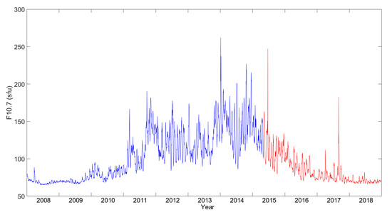
Figure 1.
The F10.7 index from 2008–2018.
The COSMIC post-processed level2 ionPrf format data were downloaded from CDAAC at UCAR (https://data.cosmic.ucar.edu/ accessed on 1 October 2021). The F layer peak parameters, NmF2 and hmF2, were directly retrieved from the ionPrf format data. We used the data from the post-processed database in which the data were corrected, and the extremely bad profiles were eliminated [29].
At the Ganzi station, routine ionospheric vertical sounding was performed by an ionosonde called the Chinese Academy of Sciences Digital Ionosonde System (CAS-DIS) from May 2015 to present. The CAS-DIS works in the frequency range of 1 MHz to 26 MHz, with the steps of 0.05 MHz and a range resolution of 5 km [30]. The ionosonde transmits and receives digital signals every 15 min; therefore, there are ninety-six ionograms every day. SAO Explorer software, developed by the University of Massachusetts Lowell, was applied to scale the ionograms, and the ARTIST algorithm embedded in the software was used to obtain the ionospheric electron density profile [28]. We scaled every ionogram manually to avoid poor automatic scaling due to inadequate quality of the ionogram or an unpredictable situation. During the manual scaling, the ionograms with low signal-to-noise ratios or strong spread-F were eliminated.
We used the COSMIC electron density profile in the selected region, which is a rectangle area of 5° in latitude and 10° in longitude with its center at the Ganzi station (31.2° N, 100.4° E), to compare the electron density profile data from the ionosonde observations at that station, as shown in Figure 2. The maximum time difference between the selected data pairs was ±7.5 min. The fitting was restricted to the altitude range of 200–400 km to avoid a larger error at lower altitudes [27]. The number of eligible data pairs of COSMIC and ionosonde data was 296. Figure 3 shows the temporal distribution of the selected data pairs. Because of the lack of COSMIC RO data, the pairs number reduced obviously in 2017 and 2018. As for the distribution of data pairs in local hours, the number of data pairs was much less during the afternoon, especially at 12:00 LT.
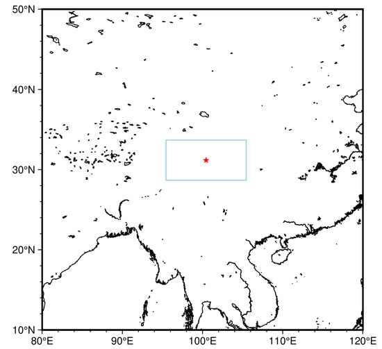
Figure 2.
The ionosonde’s location and the selected region of the COSMIC observations. The red star denotes the ionosonde at Ganzi (31.2° N, 100.4° E), while the 5° × 10° rectangle is the selected region of the COSMIC tangent point.
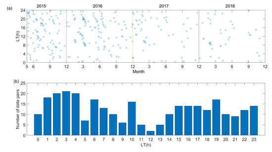
Figure 3.
(a) The temporal distribution of selected data pairs, in which one circle means one data pair; (b) the number of selected data pairs in 1 h local time bins.
In order to study the correlation of two kind of techniques, the least squares method was applied to fit the selected data pairs. The formula of the fitting curve is as follows:
where is the value of the NmF2 or hmF2 obtained from the ionosonde, is the value of the NmF2 or hmF2 obtained from the COSMIC, and and are fitting coefficients.
Furthermore, the correlation coefficient between the selected data pairs is calculated by the following:
where is the correlation coefficient of selected data pairs, is the number of selected data pairs, is the value of the NmF2 or hmF2 obtained from the ionosonde, is the average value of , is the value of the NmF2 or hmF2 obtained from COSMIC, and is the average value of .
3. Results
In this section, we compare the parameters obtained from the COSMIC measurements and ionosonde observations. The electron density profiles obtained from an individual COSMIC RO event and corresponding ionosonde observation are presented. Then, the comparison of the NmF2 and hmF2 from selected data pairs at different local times in different seasons is presented.
Figure 4 shows the comparison of an individual COSMIC RO event and corresponding ionosonde observation. The maximum electron density of COSMIC RO occurred on 16 October 2015 at 01:44 UT (09:44 LT), while the corresponding ionogram recorded by the ionosonde occurred on 16 October 2015 at 01:45 UT (09:45 LT). The position of the COSMIC RO maximum electron density is at 32.8° N, 100.9° E, which is close to the Ganzi station (31.2° N, 100.4° E).
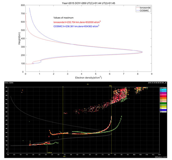
Figure 4.
Comparison of the electron density profile retrieved from the COSMIC measurement and the ionosonde observation on 16 October 2015 at 01:44 UT (09:44 LT). The corresponding ionogram recorded on 16 October 2015 at 09:45 LT.
The NmF2 obtained from the COSMIC and ionosonde are 8.34 × 10⁵ el/cm3 and 8.32 × 10⁵ el/cm3. The hmF2 obtained from the COSMIC and ionosonde are 236.381 km and 232.704 km. The differences between the parameters obtained from two kinds of techniques are very small. Thus, the COSMIC electron density profile and ionosonde electron density profile are in good agreement between 150 km to 350 km. We also notice that the electron density retrieved from the COSMIC measurements is much larger than the electron density retrieved from the ionosonde observations above 350 km. The reason needs further exploration, and the topic is out of the scope of this paper.
In the following, we compare the parameters from selected data pairs at different local times in different seasons. As mentioned in Section 2, the maximum time difference of selected data pairs is ±7.5 min, and the maximum difference in latitude and longitude are ±2.5° and ±5°. All eligible data pairs between the May 2015 to December 2018 were used.
Figure 5 shows the comparison of the parameters obtained from the COSMIC measurements and ground-based ionosonde observations. The number of data pairs in the comparison is 296. The correlation coefficient of the NmF2 and hmF2 are 0.94 and 0.77, respectively. These values confirm the strong positive correlation between the COSMIC measurements and ground-based ionosonde observations. The retrieved electron density profiles from the COSMIC measurements could provide a slightly overestimated value when we compared them with those derived from ionosonde observations.
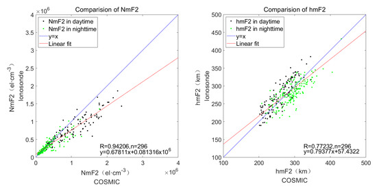
Figure 5.
Comparison of the values of the NmF2 (left) and hmF2 (right) obtained from the COSMIC and ionosonde. Black dots are NmF2 and hmF2 in the daytime (07:00–18:00 LT). Green dots are NmF2 and hmF2 in the nighttime (19:00–06:00 LT). The red line is a linear fit to all data points. The blue line represents y = x.
Then, the selected data pairs were divided into two groups: daytime (07:00–18:00 LT) and nighttime (19:00–06:00 LT). Table 1 shows the correlation of the NmF2 and hmF2 retrieved from the COSMIC measurements and ground-based ionosonde observations at different local times. The number of data pairs of daytime and nighttime are 121 and 175. The correlation coefficient of the NmF2 is 0.92 during the daytime and 0.88 during the nighttime. The correlation coefficient of the hmF2 is 0.87 during the daytime and 0.77 during the nighttime. It is obvious that the correlation of the NmF2 and hmF2 are both stronger during the daytime than during the nighttime.

Table 1.
Correlation coefficient of the NmF2 and hmF2 in the daytime (07:00 LT–18:00 LT) and nighttime (19:00 LT–06:00 LT).
Furthermore, the correlation of the parameters in different seasons, namely, summer (May to August), winter (November to February), and equinox (March to April and September to October), is also investigated. Figure 6 shows the NmF2 and hmF2 from COSMIC measurements and ionosonde observations in different seasons. Table 2 shows the correlation coefficients of the parameters between the COSMIC measurements and ionosonde observations in different seasons. The number of selected data pairs in the summer, winter, and equinox are 117, 75, and 105, respectively. The correlation coefficient of the NmF2 is highest during the winter and lowest during the summer, while the correlation coefficient of the hmF2 is highest during the equinox and lowest during the summer. In general, the differences of correlation coefficients of the NmF2 and hmF2 during three seasons are small.
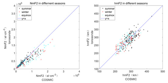
Figure 6.
Nmf2 (left) and hmF2 (right) from the COSMIC measurements and ionosonde observat–ions in different seasons.
Table 2.
Correlation coefficient of the NmF2 and hmF2 in different seasons.
Moreover, hourly values for the NmF2 and hmF2 were averaged from selected pairs of data, with a time difference of less than 30 min from a given hour. Figure 7 shows the hourly variations of the NmF2 and hmF2 retrieved from the COSMIC measurements and ionosonde observations at different local times. The results show that COSMIC tends to overestimate NmF2 except in the morning (03:00–08:00 LT). In addition, the discrepancy of the NmF2 is maximum at noon. The larger the value of the NmF2, the larger the discrepancy between two kinds of measurements. The COSMIC tends to underestimate the hmF2 during the afternoon (10:00–20:00 LT) and overestimate the hmF2 during the morning (21:00–09:00 LT).
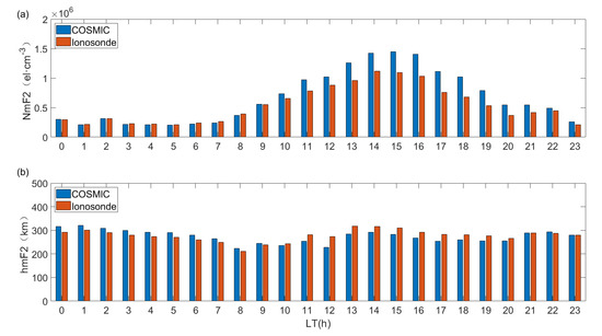
Figure 7.
Hourly NmF2 (a) and hourly hmF2 (b) of local time obtained from the COSMIC measur–ements and ionosonde observations.
4. Discussion
In the COSMIC electron density profile inversion, the Abel transformation and the spherical symmetry assumption are adopted [31]. On the other hand, the ARTIST technique, embedded in SAO Explorer software, is used to convert the ionosonde observations from virtual heights to real heights [32]. Therefore, the validation of the COSMIC measurements at the mid-latitude region of China is necessary.
The electron density profiles obtained from an individual COSMIC RO event and the corresponding ionosonde observation at the Ganzi station showed great consistency, and former works have similar results. A comparison of an electron density profile obtained from the COSMIC and ionosonde observations over Cachoeira Paulista (22.7° S, 45.0° W) in Brazil (longitude difference is about 3.5°, and latitude difference is less than 2.5°) showed very good agreement for almost the entire profile [29]. A comparison of an electron density profile from the COSMIC and ionosonde observations at Sanya (18.3° N, 109° E) also presented good agreement, while the electron density obtained from the COSMIC is much larger than that from the ionosonde above 400 km [28]. The unconformity might be caused by the SAO Explorer software topside electron density profile algorithm ARTIST, which uses the parameter at the F layer peak with a steady scale height to calculate the topside electron density profile [33]. Additionally, it could be due to the COSMIC RO electron density profile retrieval error as the error is significant when approaching the orbit of low-Earth orbit satellites. A notable feature is that the RO estimation method tends to overestimate the electron density by ~10% systematically. It can be concluded that ~60% deviations are located between −10% and 30%. The overestimation might be due to the approximation of constant electron density around the orbit used in our RO estimation method since the electron density always decreases with the increase of altitude in the topside ionosphere [31].
As for the selected data pairs, the correlation of the NmF2 obtained from the COSMIC measurements and ionosonde observations is much stronger than the correlation of the hmF2, which is similar to the results at Zuoling station. The correlation coefficients of the NmF2 and hmF2 obtained from the COSMIC measurements and ground-based ionosonde observations at the Zuoling (31.00° N, 114.5° E) station during maximum solar activity are 0.89 and 0.67, respectively [34].
In our work, the correlation of the parameters is stronger during the daytime than during the nighttime. The correlation coefficients of the NmF2 between the COSMIC measurements and ionosonde observations at Jicamarca (12° S, 283° W) are slightly better at nighttime than at daytime in different seasons. It is worth noting that the Jicamarca station is near the magnetic equator, so the electron density profiles obtained from the COSMIC measurements would be significantly enhanced when the equatorial ionization anomaly (EIA) appears [35]. In addition, the correlation coefficient of the hmF2 is highest during the equinox over Ascension Island, which is consistent with the result of this paper [36].
Chu et al. conducted a global survey of comparison between the COSMIC measurement and ground-based ionosonde observation, and the results showed that average peak densities from the COSMIC measurements were constantly smaller than those from the ionosonde observations except at a latitude of 30° N [32]. As Figure 7 shows, the value of the hourly NmF2 obtained from COSMIC measurements is constantly larger than those obtained from ionosonde observations at the Ganzi station, especially at noon when the value of the hourly NmF2 is large.
5. Conclusions
In the present paper, the COSMIC measurements are validated by ground-based ionosonde observations over Ganzi during low solar activity from May 2015 to December 2018. First, an individual example was presented to analyze the consistency of an electron density profile obtained from the COSMIC measurements and ionosonde observations. Then, the correlation of the parameters obtained from the selected data pairs was investigated at different local times in different seasons. The major findings are summarized as follows:
- The correlation coefficients of the parameters (including NmF2 and hmF2) from two kinds of techniques are 0.94 and 0.77. The COSMIC measurements are consistent with the ionosonde observations near the Ganzi Station (31.2° N, 100.4° E). It means the COSMIC measurements are valid in the middle latitude of China during low solar activity from May 2015 to December 2018. The COSMIC measurements will be useful in the further ionospheric research in this region.
- The correlation coefficients of the NmF2 from these data pairs are larger than those of the hmF2 at different local times. The consistency may be due to the Abel inversion in the COSMIC data processing and the algorithm embedded in the SAO Explorer software.
- The correlation coefficients of the parameters (including NmF2 and hmF2) are larger in the daytime than those at night. The differences of correlation coefficients of the parameters (including NmF2 and hmF2) in all seasons are small.
- The NmF2 from COSMIC is overestimated during the whole day except in the morning (03:00–08:00 LT). The hmF2 from COSMIC is overestimated in the morning (10:00–20:00 LT) and underestimated in the afternoon (21:00–09:00 LT).
- The larger the value of the NmF2, the larger the discrepancy of the NmF2 is between the two kinds of techniques.
Author Contributions
Conceptualization, L.H. and F.S.; methodology, L.H.; software, X.L.; validation, L.H., F.S. and F.Z.; formal analysis, X.L.; investigation, L.H.; writing—original draft preparation, L.H.; writing—review and editing, F.S.; visualization, X.L.; supervision, F.Z. All authors have read and agreed to the published version of the manuscript.
Funding
This research was funded by the APSCO (Asia-Pacific Space Cooperation Organization) Earthquake Research Project Phase II: Integrating Satellite and Ground Observations for Earthquake Signatures and Precursors, grant number WX0519502.
Data Availability Statement
Not applicable.
Acknowledgments
We appreciate UCAR for providing COSMIC data online through CDAAC.
Conflicts of Interest
The authors declare no conflict of interest.
References
- Rocken, C.; Anthes, R.; Exner, M.; Hunt, D.; Sokolovskiy, S.; Ware, R.; Gorbunov, M.; Schreiner, W.; Feng, D.; Herman, B. Analysis and validation of GPS/MET data in the neutral atmosphere. J. Geophys. Res. 1997, 102, 29849–29866. [Google Scholar] [CrossRef]
- Hajj, G.A.; Romans, L.J. Ionospheric electron density profiles obtained with the Global Positioning System: Results from the GPS/MET experiment. Radio Sci. 1998, 33, 175–190. [Google Scholar] [CrossRef]
- Liu, L.; Wan, W.; Ning, B.; Zhang, M.L.; He, M.; Yue, X. Longitudinal behaviors of the IRI-B parameters of the equatorial electron density profiles retrieved from FORMOSAT-3/COSMIC radio occultation measurements. Adv. Space Res. 2011, 46, 1064–1069. [Google Scholar] [CrossRef]
- Zhao, B.; Wan, W.; Yue, X.; Liu, L.; Liu, J. Global characteristics of occurrence of an additional layer in the ionosphere observed by COSMIC/FORMOSAT-3. Geophys. Res. Lett. 2011, 38, L02101. [Google Scholar] [CrossRef]
- Lin, C.H.; Hsiao, C.C.; Liu, J.Y.; Liu, C.H. Longitudinal structure of the equatorial ionosphere: Time evolution of the four-peaked EIA structure. J. Geophys. Res. 2007, 112, A12305. [Google Scholar] [CrossRef]
- Lin, C.H.; Liu, J.Y.; Fang, T.W.; Chang, P.Y.; Tsai, H.F.; Chen, C.H.; Hsiao, C.C. Motions of the equatorial ionization anomaly crests imaged by FORMOSAT-3/COSMIC. Geophys. Res. Lett. 2010, 34, L19101. [Google Scholar] [CrossRef]
- Lin, C.H.; Wang, W.; Hagan, M.E.; Hsiao, C.C.; Immel, T.J.; Hsu, M.L.; Liu, J.Y.; Paxton, L.J.; Fang, T.W.; Liu, C.H. Plausible effect of atmospheric tides on the equatorial ionosphere observed by the FORMOSAT-3/COSMIC: Three-dimensional electron density structures. Geophys. Res. Lett. 2007, 34, 224–238. [Google Scholar] [CrossRef]
- Ram, S.T.; Su, S.Y.; Liu, C.H.; Reinisch, B.W.; Mckinnell, L.A. Topside ionospheric effective scale heights (HT) derived with ROCSAT-1 and ground-based ionosonde observations at equatorial and midlatitude stations. J. Geophys. Res. 2010, 114, A10309. [Google Scholar]
- Schreiner, W.S.; Sokolovskiy, S.V.; Rocken, C. Analysis and validation of GPS/MET radio occultation data in the ionosphere. Radio Sci. 1999, 34, 949–966. [Google Scholar] [CrossRef]
- Kuo, Y.H.; Sokolovskiy, S.V.; Anthes, R.A.; Vandenberghe, F. Assimilation of GPS Radio Occultation Data for Numerical Weather Prediction. Terr. Atmos. Ocean. Sci. 2001, 11, 157. [Google Scholar] [CrossRef]
- Syndergaard, S. On the ionosphere calibration in GPS radio occultation measurements. Radio Sci. 2016, 35, 865–884. [Google Scholar] [CrossRef]
- Beyerle, G. GPS radio occultation with GRACE: Atmospheric profiling utilizing the zero difference technique. Geophys. Res. Lett. 2005, 32, L13086. [Google Scholar] [CrossRef]
- Hajj, G.A.; Ao, C.O.; Iijima, B.A.; Kuang, D.; Yunck, T.P. CHAMP and SAC-C atmospheric occultation results and intercomparisons. J. Geophys. Res. 2004, 109, D06109. [Google Scholar] [CrossRef]
- Jakowski, N.; Wehrenpfennig, A.; Heise, S.; Reigber, C.; Lühr, H.; Grunwaldt, L.; Meehan, T.K. GPS radio occultation measurements of the ionosphere from CHAMP: Early results. Geophys. Res. Lett. 2002, 29, 1450–1457. [Google Scholar] [CrossRef]
- Wickert, J.; Reigber, C.; Beyerle, G.; Knig, R.; Hocke, K. Atmosphere sounding by GPS radio occultation: First results from CHAMP. Geophys. Res. Lett. 2001, 28, 3263–3266. [Google Scholar] [CrossRef]
- Fong, C.J.; Shiau, W.T.; Lin, C.T. Constellation Deployment for the FORMOSAT-3/COSMIC Mission. IEEE Trans. Geosci. Remote Sens. 2008, 46, 3367–3379. [Google Scholar] [CrossRef]
- Fong, C.J.; Yang, S.K.; Chu, C.H.; Huang, C.Y.; Yeh, J.J.; Lin, C.T.; Kuo, T.C.; Liu, T.Y.; Yen, N.L.; Chen, S.S. FORMOSAT-3/COSMIC Constellation Spacecraft System Performance: After One Year in Orbit. IEEE Trans. Geosci. Remote Sens. 2008, 48, 3380–3394. [Google Scholar] [CrossRef]
- Liu, L.; He, M.; Wan, W.; Zhang, M.L. Topside ionospheric scale heights retrieved from Constellation Observing System for Meteorology, Ionosphere, and Climate radio occultation measurements. J. Geophys. Res. 2008, 113, A10304. [Google Scholar] [CrossRef]
- Liu, L.; Le, H.; Chen, Y.; He, M.; Yue, X. Features of the middle- and low-latitude ionosphere during solar minimum as revealed from COSMIC radio occultation measurements. J. Geophys. Res. 2012, 116, A09307. [Google Scholar] [CrossRef]
- Liu, L.; Zhao, B.; Wan, W.; Ning, B.; Zhang, M.L.; He, M. Seasonal variations of the ionospheric electron densities retrieved from Constellation Observing System for Meteorology, Ionosphere, and Climate mission radio occultation measurements. J. Geophys. Res. 2009, 114, A02302. [Google Scholar] [CrossRef]
- Wickert, J.; Michalak, G.; Schmidt, T.; Beyerle, G.; Cheng, C.Z.; Healy, S.B.; Heise, S.; Huang, C.Y.; Jakowski, N. GPS Radio Occultation: Results from CHAMP, GRACE and FORMOSAT-3/COSMIC. Terr. Atmos. Ocean. Sci. 2009, 20, 35–50. [Google Scholar] [CrossRef]
- Luan, X.; Wang, W.; Burns, A.; Solomon, S.C.; Lei, J. Midlatitude nighttime enhancement in F region electron density from global COSMIC measurements under solar minimum winter condition. J. Geophys. Res. 2008, 113, A09319. [Google Scholar] [CrossRef]
- Zakharenkova, I.E.; Krankowski, A.; Shagimuratov, I.I.; Cherniak, I.V.; Lagovsky, A.F. Use of FORMOSAT-3 / COSMIC for observation of the ionospheric storm effects on October 11, 2008. Earth Planets Space 2012, 64, 505–512. [Google Scholar] [CrossRef][Green Version]
- Huang, X.; Reinisch, B.W. Vertical electron density profiles from the Digisonde network. Adv. Space Res. 1996, 18, 121–129. [Google Scholar] [CrossRef]
- Lei, J.; Syndergaard, S.; Burns, A.G.; Solomon, S.C.; Wang, W.; Zeng, Z. Comparison of COSMIC ionospheric measurements with ground-based observations and model predictions: Preliminary results. J. Geophys. Res. 2007, 112, A07308. [Google Scholar] [CrossRef]
- Chuo, Y.J.; Lee, C.C.; Cheng, W.S.; Reinisch, B.W. Comparison between bottomside parameters retrieved from FORMOSAT3 measurements and ground-based observations collected at Jicamarca. J. Atmos. Terr. Phys. 2012, 73, 1665–1673. [Google Scholar] [CrossRef]
- Yue, X.; Schreiner, W.S.; Lei, J.; Sokolovskiy, S.V.; Rocken, C.; Hunt, D.C.; Kuo, Y.H. Error analysis of Abel retrieved electron density profiles from radio occultation measurements. Ann. Geophys. 2010, 28, 217–222. [Google Scholar] [CrossRef]
- Hu, L.; Ning, B.; Liu, L.; Zhao, B.; Chen, Y.; Li, G. Comparison between ionospheric peak parameters retrieved from COSMIC measurement and ionosonde observation over Sanya. Adv. Space Res. 2014, 54, 929–938. [Google Scholar] [CrossRef]
- Ely, C.V.; Batista, I.S.; Abdu, M.A. Radio occultation electron density profiles from the FORMOSAT-3/COSMIC satellites over the Brazilian region: A comparison with Digisonde data. Adv. Space Res. 2012, 49, 1553–1562. [Google Scholar] [CrossRef]
- Wang, S.; Chen, Z.; Feng, Z.; Fang, G. The new CAS-DIS digital ionosonde. Ann. Geophys. 2013, 56, R0107. [Google Scholar] [CrossRef]
- Yue, X.; Schreiner, W.S.; Rocken, C.; Kuo, Y.H. Evaluation of the orbit altitude electron density estimation and its effect on the Abel inversion from radio occultation measurements. Radio Sci. 2011, 46, RS1013. [Google Scholar] [CrossRef]
- Chu, Y.H.; Su, C.L.; Ko, H.T. A global survey of COSMIC ionospheric peak electron density and its height: A comparison with ground-based ionosonde measurements. Adv. Space Res. 2010, 46, 431–439. [Google Scholar] [CrossRef]
- Reinisch, B.W.; Huang, X. Deducing topside profiles and total electron content from bottomside ionograms. Adv. Space Res. 2001, 27, 23–30. [Google Scholar] [CrossRef]
- Sun, L.F.; Zhao, B.Q.; Yue, X.A.; Mao, T. Comparison between ionospheric character parameters retrieved from FORMOSAT3 measurement and ionosonde observation over China. Chin. J. Geophys. 2014, 57, 3625–3632. [Google Scholar]
- Liu, J.Y.; Lee, C.C.; Yang, J.Y.; Chen, C.Y.; Reinisch, B.W. Electron density profiles in the equatorial ionosphere observed by the FORMOSAT-3/COSMIC and a digisonde at Jicamarca. GPS Solut. 2010, 14, 75–81. [Google Scholar] [CrossRef]
- Chuo, Y.J.; Lee, C.C.; Chen, W.S.; Reinisch, B.W. Comparison of the characteristics of ionospheric parameters obtained from formosat-3 and digisonde over Ascension Island. Ann. Geophys. 2013, 31, 787–794. [Google Scholar] [CrossRef]
Publisher’s Note: MDPI stays neutral with regard to jurisdictional claims in published maps and institutional affiliations. |
© 2022 by the authors. Licensee MDPI, Basel, Switzerland. This article is an open access article distributed under the terms and conditions of the Creative Commons Attribution (CC BY) license (https://creativecommons.org/licenses/by/4.0/).