Abstract
It is conjectured that in cosmological applications the particle current is not modified but finite heat or energy flow. Therefore, comoving Eckart frame is a suitable choice, as it merely ceases the charge and particle diffusion and conserves charges and particles. The cosmic evolution of viscous hadron and parton epochs in casual and non-casual Eckart frame is analyzed. By proposing equations of state deduced from recent lattice QCD simulations including pressure p, energy density , and temperature T, the Friedmann equations are solved. We introduce expressions for the temporal evolution of the Hubble parameter , the cosmic energy density , and the share and the bulk viscous coefficient . We also suggest how the bulk viscous pressure could be related to H. We conclude that the relativistic theory of fluids, the Eckart frame, and the finite viscous coefficients play essential roles in the cosmic evolution, especially in the hadron and parton epochs.
Keywords:
observational cosmology; mathematical and relativistic aspects of cosmology; quark-gluon plasma PACS:
98.80.Es; 98.80.Jk; 12.38.Mh
1. Introduction
Giving a reliable description for matter and/or radiation filling in the cosmological background geometry, the space, is an essential ingredient to determine the temporal evolution of the Universe. A realistic picture of the cosmic evolution can only be drawn, if reliable equations of state could be proposed. Since no observational evidence of the cosmic evolution, especially during the very early epochs of the Universe, was made so far, we first have to do the best of all in order to best describe the cosmic matter and/or radiation [1].
Recent perturbative and non-perturbative lattice simulations with almost all quark flavors and thermal contributions from charged leptons, electroweak particles, scalar Higgs bosons, and photons have calculated various thermodynamic quantities like pressure, energy density, bulk viscosity, relaxation time, and temperature up to the TeV-scale [2]. Therefore, an access to the relativistic dissipative cosmic fluid covering hadron, QGP, and electroweak (EW) epochs is likely gained. On the other hand, the shear viscosity could be originated to curvature effects through Ricci tensor or Ricci scalar of a given spacetime, for example, some radiation processes from an accretion disk may attribute to shear viscosity and heat flow. The exponential expansion of the Universe significantly contributes to the curvature effects in the bulk viscosity.
An approach for relativistic hydrodynamics has found applications in various disciplines, especially in physics of the early Universe [3,4,5]. For ideal fluids, the theory of hydrodynamics was first formulated by Euler [6]. This was much later extended to non-ideal fluids by Navier [7] and Stokes [8] and utilized in determining dissipative quantities like viscosity and heat flow.
About eight decades ago, the relativistic theory of fluids was introduced by Eckart [9] and Landau–Lifshitz [10], in which the relativistic version of Euler ideal and Navier-Stokes non-ideal fluids was developed. The latter is characterized by first-order gradients of the hydrodynamical variable, i.e., the dissipative quantities are constructed from the first-order gradients of the fluid’s four-velocity, temperature, and chemical potential. But it was ascertained that the dissipative perturbation has infinite speed [11,12,13,14]. A linear relation between the bulk viscous pressure and the expansion in the early Universe was also suggested [5].
Hiscock and Lindblom pointed out that under linear perturbations the relativistic theory for non-ideal fluids suffers from instabilities and allows a non-casual signal propagation [15]. It was also found that the dissipative quantities seem to instantaneously response to the first-order changes in Eckart and Landau–Lifshitz theory. When repairing this in light of the theory of general relativity, Mueller [16] and Israel–Stewart [17,18] came up with a causal theory which is stable under linear perturbations and the dissipative perturbation has finite speed [15]. Here, the second-order gradients are dominant [11,12,13].
To address phenomenology of relativistic heavy-ion collisions assuming vanishing conserved charges in Landau frame, a systematic expansion of the hydrodynamical gradients has been done in context of conformal and non-conformal theories and relativistic viscous fluids could be investigated [19,20]. Under the assumption of conserved charges and finite heat flux, Lahiri started with the second-order gradients expansion in the Eckart frame and developed a causal theory of relativistic non-ideal fluids for various astrophysical applications [14]. In other words, general relativistic causal hydrodynamical equations in the Eckart frame like of bulk viscosity, shear viscosity tensor, and heat flow are obtained up to second-order gradients.
In astrophysical and cosmological applications, where the particle current is not modified but the heat or energy flow is non-negligible, comoving Eckart frame is a suitable choice. As it merely ceases the charge and particle diffusion (conserved charges and particles of the system n are given from , where is the conserved charge/particle flux and is the four-velocity), while in the Landau frame there is no energy or heat flow (, where is the energy density and no dissipation of energy appears), where stands for four-velocity of particle motion and/or energy transport [21]. To summarize, in comoving frame of reference, the Eckart frame conserves , while the Landau frame conserves .
The present work aims at parameterizing various thermodynamical and transport quantities for the general relativistic causal hydrodynamical equations in the Eckart frame. For the first time, a cosmological implication of causal Eckart frame is presented. We focus on recent lattice QCD simulations [22]. The temporal evolution of cosmological parameters like the scale factor, the Hubble parameter, etc. is presented.
The paper is organized as follows. The Friedmann equations are reviewed in Section 2. The equations of state of viscous QCD epoch and the parameterizations for different thermodynamic properties are presented in Section 3. The resulting cosmic evolution is elaborated in Section 5. Section 6 is devoted to the conclusions.
2. Friedmann Equations in Eckart Frame
We assume that the bulk viscous fluid shapes the background geometry, the space, of the early Universe and limit to discussion to the QCD epoch. For spatially flat background geometry, the Friedmann–Lemaiture–Robertson–Walker (FLRW) line element reads [5]
where is the scale factor. The temporal evolution becomes accessible when integrating this in the theory of general relativity. Then, the Hubble parameter , where is the time evolution of the scale factor, can be estimated from the Einstein field Equations [5]
where is known as the reduced Planck mass MeV [5], is the effective thermodynamic pressure and is the energy density. Here, we use natural units with , so that . The reduced Planck time is given as MeV. Therefore, the Hubble parameter reads
and its time evolution can be deduced from Equations (2) and (3)
The temporal evolution of the energy density can be related to H [5]
To solve the field equations, various baratropic EoS including the bulk viscous pressure have to be substituted. Relating to or indirectly to H depends the features of causality and stability on the corresponding relativistic fluid theory. As discussed in introduction, the Eckart theory, which is a non-casual and unstable theory, is the relativistic version of non-viscous and viscous fluid theories introduced by Euler and Navier–Stokes, respectively.
In astrophysics and cosmology, the particle current-in contrary to heat or energy flow-likely remains unmodified. This makes the Eckart frame the suitable choice. With a second-order gradients expansion in the Eckart frame, non-causal theory of relativistic non-ideal fluids was developed for astrophysical applications [14]. This is similar to the causal stable Mueller–Israel–Stewart theory but explicitly in the Eckart frame. Various general relativistic causal hydrodynamical equations like bulk viscosity, shear viscosity tensor, and heat flow up to second-order gradients have been derived. The four-velocity normalization conditions reads and , where the projection tensor in curved spacetime is given as [14]. To summarize, the proposed Eckart and Mueller–Israel–Stewart theories are causal. While the latter considers up to the second-order derivations of the thermodynamic quantities, the earlier is limited to first order, only.
Comments of features of non-casual and causal Eckart Frame are now in order.
- Non-casual Eckart frame: The entropy current can be given as but it isn’t conserved all the time, where s is the entropy density and n is the number density. It was found that Eckart theory violates the second law of thermodynamics as a result of the divergence of the entropy current [5]. There is a linear relation between the Hubble parameter H and the bulk viscous pressure which results form the first-order derivations of the equilibrium states [5]where is the bulk viscosity coefficient.
- Causal Eckart frame: To avoid violating the causality principle, higher-order deviations from the equilibrium states are taken into consideration, mostly the second-order derivations of the thermodynamic quantities [14]. Using gradient expansion scheme of fluid hydrodynamical variables, the causality preserving property of the theory could be defined. The Mueller–Israel–Stewart theory, which is second-order theory in gradients of fluid hydrodynamical variables gives rise to causal and stable theory of viscous hydrodynamics. By using gradient expansion scheme up to second order and keeping the spirit of Mueller–Israel–Stewart theory, non-causal stable theory of relativistic non-ideal fluids in the Eckart frame was developed [14]. By solving the continuity equation, the modified Friedmann equation and the evolution equation of the bulk viscosity, the effects of chemical potential can be studied. Accordingly, the structure of bulk viscosity up to second-order gradients is given asThe first line in rhs gives the first-order gradient terms. The other lines list out the possible second-order gradient terms for scalars, vectors and tensors constructing the dissipative flux quantities. T is temperature, is chemical potential, , and .
3. Equations of State of Viscous QCD Matter
The lattice QCD simulations are based on non-perturbative solution of the quantum chromodynamics (QCD) theory of the strong interactions. In high energy physics, the colored parton phase, the quark-gluon plasma, which is likely created in the relativistic collisions [23,24], is conjectured to expand with a fixed number of both baryon number and entropy, so the ratio entropy/baryon number remains constant, . For each ratio, the phase diagram, T-, is obtained and also an EoS can be deduced. For the lattice simulations 4-stout improved staggered fermions with temporal lattice sizes 10, 12, and 16 with physical quark masses. are used. An isospin symmetry is assumed. Describing the state of the system of interest relies on EoS proposed; thermodynamic properties like pressure p, density , and temperature T.
From recent lattice QCD calculations, at non-vanishing baryon chemical potential [22], different EoS could be derived. As presented in Figure 1, we parameterize the results as follows.
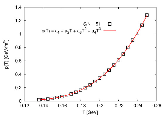
Figure 1.
Pressure p is given in dependence on the temperature T. The symbols refer to lattice QCD simulations [22] and the solid curve stands for the proposed expression, Equation (9).
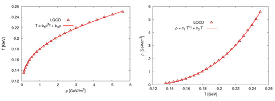 Figure 2. Left-hand panel depicts the temperature T in dependence on the energy density . The right-hand panel shows the energy density is shown in dependence on the temperature T. The symbols are lattice QCD calculations [22] and the solid curves represent to the proposed expressions, Equations (10) and (11), respectively.
- Then, the baratropic EoS can be given aswhere and , Figure 3.
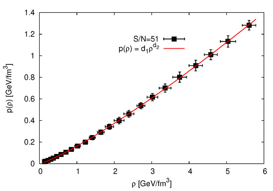 Figure 3. Pressure p is drawn in dependence on the energy density . Symbols are lattice QCD calculations along trajectories of constant [22]. The solid curve refers to the statistical fit, Equation (12).
 - For speed of sound squared vs. Twhere , , and . The speed of sound squared can be derived as .
- For vs. ratio of bulk to shear viscositywhich is based on kinetic model [25], Figure 4. Then, the temperature dependence of the ratio of shear to bulk viscosity can be parameterized aswhere , and .
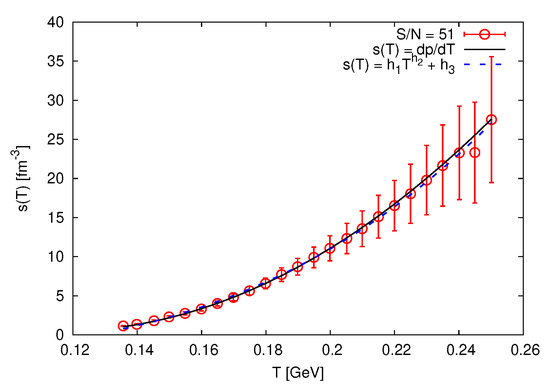
- For entropy density s vs. T
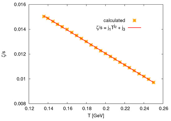
- For bulk viscosity normalized to entropy vs. Twhere [25]. The results are depicted in Figure 6. The results can be best fitted aswhere , , and .
- Then, for vs. Twhere the entropy density is substituted from Equation (16) into Equation (18). Figure 7 shows our calculations, Equation (20), as a solid curve. The results can be fitted,where , , , and .
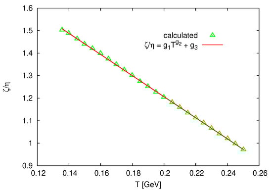
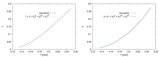 Figure 7. Left-hand panel depicts as a function of T. Our calculations is shown as a solid curve, Equation (20), while the dashed curve is Equation (21). The right-hand panel gives as a function of T. Our calculations is depicted as the solid curve, Equation (22), while the dashed curve shows results from Equation (23).
4. Evolution of the Cosmic Parameters
At Bag pressure MeV, we plot in Figure 8 data taken from ref. [5] for the time evolution of the temperature. This can be parameterized as
where , , and . An expression for t vs. T is suggested as
where is the reduced Planck time GeV.
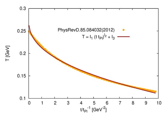
Figure 8.
Time dependence of the temperature T, at the bag constant MeV, on time t. The symbols refer to the results.
- When integrating over the comoving time t, we getThe results are depicted as symbols in Figure 9. These results can then be fitted as (solid curve in Figure 10)where , , , and .
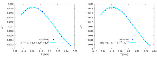 Figure 10. The left panel shows the time evolution of the scale factor during the quark-hadron phase transition, at bag constant MeV. The solid curve presents our fit to Equation (29). The right panel depicts the scale factor as a function of T, Equation (30), while solid curve presents Equation (31).
 - The calculations from this expression are depicted as symbols in Figure 10. The solid curve refers to the proposed expressionwhere , , , and .
- The time evolution of the Hubble parameter can be deduced as follows. First we substitute T from Equation (24) into Equation (26)Second, we differentiate the previous expression wrt tThe results are shown as solid curve in Figure 11.
- For the time evolution of the energy density, we first substitute T from Equation (24) into Equation (11)Then, we differentiate this equation wrt tThe resulting are depicted as a solid curve in Figure 11.
- We calculate by substituting , H, , and p into Equation (40). The results are plotted as squares in Figure 12. in the non-casual Eckart frame, Equation (7), is presented as circles. From statistical fit, we proposewhich is presented as a solid curve in Figure 10, where , , and .
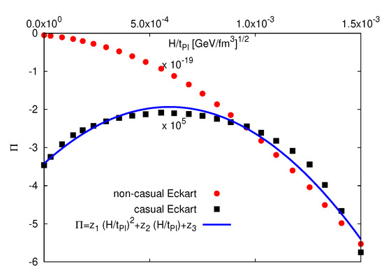 Figure 12. in dependence on H. Circle symbols refer to calculations using non-casual Eckart theory while square symbols refer to calculations using casual Eckart theory. Solid curve refers to the proposed expression for the dependence of on H.
5. Results
Figure 1 shows the dependence of the pressure p on the temperature T. The symbols refer to the lattice QCD calculations [22] and the solid curve gives to the proposed expression, Equation (9). There is an excellent agreement. We find that increasing T leads to a rapid increase in p. This characterizes a phase transition from confined hadron to deconfined parton phase [23,24]. The condition for the transition from hadron to parton epoch is the temperature, where the density is conjectured to remain small.
The left-hand panel of Figure 2 depicts the temperature T as a function of the energy density . The right-hand panel presents the dependence of the energy density on the temperature T. The symbols refer to lattice QCD calculations [22] and the solid curve stand for the proposed expressions, Equations (10) and (11), respectively. We find that T largely increases with , and also increases with T. As concluded for p, can be taken as an order parameter. It should be noted that the hadron-parton transition is not discontinuous. It is known as a rapid crossover.
Figure 3 presents the dependence of the pressure p on the energy density . The symbols with errorbars are the lattice QCD calculations along trajectories of constant ratio of entropy to particle number, [22]. The solid curve refer to the proposed EoS, Equation (12). We find that p increases as increases. Such a dependence slightly varies when moving from hadron to parton phase. The results on the speed of sound squared, which also expresses the EoS obtained, are depicted in Figure 13.
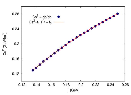
Figure 13.
Speed of sound squared is given in dependence on the temperature T. The symbols are the lattice QCD calculations [22]. The solid curve represents Equation (20).
Figure 4 presents the ratio of bulk to shear viscosity as a function of T. The symbols refer to calculations from Equation (14) [25], while the solid curve shows the fitting according to Equation (15). We find that is inversely linearly proportional to T.
To determine the ratio in dependence on T, we first determine the dependence of the entropy density s on T. Figure 5 depicts s as a function of T. The symbols depict the lattice QCD calculations evaluated from Equation (16). The solid curve refers to the proposed expression, Equation (17). We notice that s increases with the increase in T. Similar to p and , s acts as an order parameter differentiating between confined (hadron) and deconfined (parton) phases. Accordingly, we conclude that the local law of thermodynamics is not violated, as s is always positive. This apparently refers to casual Eckart theory [5].
Figure 6 shows the ratio as a function of T. The symbols stand for the calculations from Equation (18) which are based on Ref. [25], while the solid curve represents Equation (19). We notice that is inversely linearly proportional to T.
Figure 7 depicts the dependence of the both types of viscosity on the temperature. The left-hand panel shows the bulk viscosity as a function of T. Our calculations is depicted as a solid curve using Equation (20), while the dashed curve gives the statistical fit, Equation (21). The right-hand panel presents the shear viscosity as a function of T. Our calculations is depicted as the solid curve using Equation (22), while the dashed curve shows the statistical fit, Equation (23). We find that both viscosity coefficients rapidly increase with the increase in T, Equations (21) and (23). From the dependence of time t on temperature T, Figure 8, we can conclude that and are inversely proportional to t. This agrees well with the conclusion drawn in Ref. [5].
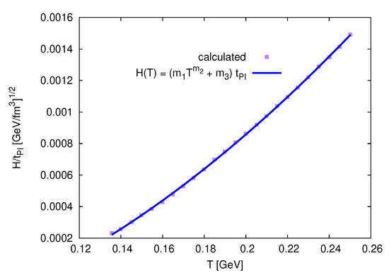
Figure 8 shows the time dependence of the temperature T, at the bag constant MeV. The symbols refer to results taken from Ref. [5], while the solid curve presents their statistical fit, Equation (24). This expression is crucial for further calculations. Figure 9 depicts the temperature dependence of the Hubble parameter H, Equation (4). The solid curve represents the statistical fit to Equation (26).
The left–hand panel of Figure 10 shows the time evolution of the scale factor during the quark-hadron phase transition, at bag constant MeV. The numerical values of the scale factors raise with increasing B, Equation (28). The solid curve presents Equation (29). We notice that rapidly increases with the increase in t. Then, begins to decrease with increasing t. At small t, rapidly increases. This means that the viscous Universe, during QCD epoch, was likely rapidly expanding. But, with the increase in t, the bulk viscosity increases. This shrinks [5]. The right-hand panel of Figure 10 depicts the scale factor as a function of the temperature T, Equation (30). The solid curve presents our fit to Equation (31). We find that increases with the increase in the temperature. Then, at MeV, begins to decrease with the increasing in T. This results from the high increasing in with the increase in T, which slows down the Universe expansion. Therefore, the scale factor likely decreases, at high temperature.
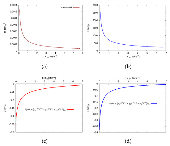
Figure 11 depicts the time evolution of the cosmological parameters , , , and . The solid curves refer to our calculations using Equations (6), (33), (36) and (38), respectively. In top panels, we find that the time evolution of and exponentially decrease with time t. This is slowing down of the Universe expansion. In bottom panels, and increase with the increasing t. This ranges from negative to positive values or is an increase in viscosity of the Universe which slows down the expansion of the Universe.
Figure 12 shows the dependence of on H. The circle symbols refer to calculations using non-casual Eckart theory [5], while squared symbols represent the calculations using casual Eckart theory. The solid curve refers to Equation (41). We notice that in non-casual Eckart theory [5] decreases with the increase in H, while in the casual Eckart theory the increase in with H is then followed by a smooth decrease forming a parabolic shape. The maximum is positioned at .
6. Conclusions
The present work aims at solving the field equations in the hadron and the parton epochs and proposing barotropic equation for the bulk viscous pressure . We solve the Friedmann equations by proposing various equations of state using recent lattice QCD simulations in the Eckart frame. While the non-casual Eckart theory violates the second law of thermodynamics so that which is defined as the covariant entropy current stemming from Gibbs equation, the causal Eckart theory-similar the the causal stable Mueller–Israel–Stewart theory-leads to general relativistic causal hydrodynamical equations in the Eckart frame such as bulk viscosity, shear viscosity tensor, and heat flow obtained up to second-order gradients.
Using recent lattice QCD simulations, we propose barotropic equations of state for hadron and parton matter. By means of statistical fits, we propose expressions for various thermodynamic quantities and cosmological parameters including , , , and . A relation between and H was introduced. The validation of the causal theory could be guaranteed. In non-casual Eckart theory, there is a linear dependence of the Hubble parameter H and the bulk viscous pressure , which results form the first-order derivations of the equilibrium state, while in causal Eckart theory, in which bulk viscosity, shear viscosity tensor, and heat flow are obtained up to second-order gradients, the causality is guaranteed.
The scale factor starts with a rapid increase with the time. Then, it begins to decrease. We conclude that the viscous Universe, during QCD epoch, was likely rapidly expanding. But, with the time, the scale factor shrinks as the bulk viscosity increases.
We also conclude that and exponentially decrease with time, i.e., slowing down of the Universe expansion. Both and increase with the time. As this ranges from negative to positive values, an increase in viscosity seems to slow down the expansion of the Universe. The dependence of shear and bulk viscosity on the expansion rate shall be investigated in a future work.
In the causal relativistic theory which conserves the charges and the particles and simultaneously allows finite heat and energy flow, the viscous pressure plays an essential role in drawing a reliable picture on the cosmic evolution of the early Universe Cosmological implications of the proposed causal Eckart frame is presented, for the first time.
Author Contributions
Conceptualization, A.N.T.; Theory, A.N.T.; Methodology, H.Y.; software, E.A.H. and A.N.; validation, A.N.T. and H.Y.; writing—original draft preparation, H.Y.; writing—review and editing, A.N.T.; project administration, A.N.T. All authors have read and agreed to the published version of the manuscript.
Funding
This research received no external funding.
Institutional Review Board Statement
Not applicable.
Informed Consent Statement
Not applicable.
Data Availability Statement
The present study did not report any data.
Conflicts of Interest
The authors declare no conflict of interest.
References
- Tawfik, A. Thermodynamics in the Viscous Early Universe. Can. J. Phys. 2010, 88, 825–831. [Google Scholar] [CrossRef]
- Tawfik, A.N.; Greiner, C. Early Universe Thermodynamics and Evolution in Nonviscous and Viscous Strong and Electroweak epochs: Possible Analytical Solutions. Entropy 2021, 23, 295. [Google Scholar] [CrossRef] [PubMed]
- Tawfik, A.; Harko, T.; Mansour, H.; Wahba, M. Dissipative Processes in the Early Universe: Bulk Viscosity. Uzb. J. Phys. 2010, 12, 316–321. [Google Scholar]
- Tawfik, A.; Wahba, M. Bulk and Shear Viscosity in Hagedorn Fluid. Ann. Phys. 2010, 522, 849–856. [Google Scholar] [CrossRef]
- Tawfik, A.; Harko, T. Quark-Hadron Phase Transitions in Viscous Early Universe. Phys. Rev. 2012, D85, 084032. [Google Scholar] [CrossRef]
- Euler, L. Principes generaux du mouvement des fluides. Mémoires De L’académie Des Sci. De Berl. 1757, 11, 274. [Google Scholar]
- Navier, C. Mémoire sur les lois du mouvement des fluides. Mémoires De L’Académie R. Des Sci. De L’Institut De Fr. 1823, 6, 389–440. [Google Scholar]
- Stokes, G.G. Mathematical and Physical Papers; Cambridge University Press: Cambridge, UK, 2009; Volume 3, p. 1901. [Google Scholar] [CrossRef]
- Eckart, C. The thermodynamics of irreversible processes. III. Relativistic theory of the simple fluid. Phys. Rev. 1940, 58, 919. [Google Scholar] [CrossRef]
- Landau, L.; Lifshitz, E. Fluid Mechanics; Butterworth-Heinemann: Oxford, UK, 1987. [Google Scholar]
- Piattella, O.F.; Fabris, J.C.; Zimdahl, W. Bulk viscous cosmology with causal transport theory. JCAP 2011, 1105, 29. [Google Scholar] [CrossRef]
- Acquaviva, G.; John, A.; Pénin, A. Dark matter perturbations and viscosity: A causal approach. Phys. Rev. 2016, D94, 043517. [Google Scholar] [CrossRef]
- Cruz, N.; González, E.; Palma, G. Exact analytical solution for an Israel–Stewart cosmology. Gen. Rel. Grav. 2020, 52, 62. [Google Scholar] [CrossRef]
- Lahiri, S. Second order causal hydrodynamics in Eckart frame: Using gradient expansion scheme. Class. Quant. Grav. 2020, 37, 075010. [Google Scholar] [CrossRef]
- Hiscock, W.A.; Lindblom, L. Generic instabilities in first-order dissipative relativistic fluid theories. Phys. Rev. D 1985, 31, 725–733. [Google Scholar] [CrossRef] [PubMed]
- Muller, I. Zum Paradoxon der Warmeleitungstheorie. Z. Phys. 1967, 198, 329–344. [Google Scholar] [CrossRef]
- Israel, W. Nonstationary irreversible thermodynamics: A Causal relativistic theory. Ann. Phys. 1976, 100, 310–331. [Google Scholar] [CrossRef]
- Israel, W.; Stewart, J.M. Transient relativistic thermodynamics and kinetic theory. Ann. Phys. 1979, 118, 341–372. [Google Scholar] [CrossRef]
- Baier, R.; Romatschke, P.; Son, D.T.; Starinets, A.O.; Stephanov, M.A. Relativistic viscous hydrodynamics, conformal invariance, and holography. JHEP 2008, 4, 100. [Google Scholar] [CrossRef]
- Romatschke, P. New Developments in Relativistic Viscous Hydrodynamics. Int. J. Mod. Phys. E 2010, 19, 1–53. [Google Scholar] [CrossRef]
- Monnai, A. Landau and Eckart frames for relativistic fluids in nuclear collisions. Phys. Rev. C 2019, 100, 014901. [Google Scholar] [CrossRef]
- Guenther, J.N.; Bellwied, R.; Borsanyi, S.; Fodor, Z.; Katz, S.D.; Pasztor, A.; Ratti, C.; Szabo, K. Recent lattice QCD results at non-zero baryon densities. PoS 2018, CPOD2017, 32. [Google Scholar] [CrossRef]
- Adamczyk, L.; Adkins, J.K.; Agakishiev, G.; Aggarwal, M.M.; Ahammed, Z.; Alekseev, I.; Aparin, A.; Arkhipkin, D.; Aschenauer, E.C.; Attri, A.; et al. Probing parton dynamics of QCD matter with Ω and ϕ production. Phys. Rev. C 2016, 93, 021903. [Google Scholar] [CrossRef]
- Adamovich, M.I.; Aggarwal, M.M.; Alexandrov, Y.A.; Amirikas, R.; Andreeva, N.P.; Badyal, S.K.; Bakich, A.M.; Basova, E.S.; Bhalla, K.B.; Bhasin, A.; et al. Fragmentation and multifragmentation of 10.6-A-GeV gold nuclei. Eur. Phys. J. A 1999, 5, 429–440. [Google Scholar] [CrossRef]
- Dusling, K.; Schäfer, T. Bulk viscosity, particle spectra and flow in heavy-ion collisions. Phys. Rev. 2012, C85, 044909. [Google Scholar] [CrossRef]
Publisher’s Note: MDPI stays neutral with regard to jurisdictional claims in published maps and institutional affiliations. |
© 2021 by the authors. Licensee MDPI, Basel, Switzerland. This article is an open access article distributed under the terms and conditions of the Creative Commons Attribution (CC BY) license (https://creativecommons.org/licenses/by/4.0/).