The Low-Temperature Expansion of the Casimir-Polder Free Energy of an Atom with Graphene

Abstract

We consider the low-temperature expansion of the Casimir-Polder free energy for an atom and graphene by using the Poisson representation of the free energy. We extend our previous analysis on the different relations between chemical potential $\mu$ and mass gap parameter m. The key role plays the dependence of graphene conductivities on the $\mu$ and m. For simplicity, we made the manifest calculations for zero values of the Fermi velocity. For $\mu >m$, the thermal correction $\sim T^2$, and for $\mu <m$, we confirm the recent result of Klimchitskaya and Mostepanenko, that the thermal correction $\sim T^5$. In the case of exact equality $\mu =m$, the correction $\sim T$. This point is unstable, and the system falls to the regime with $\mu >m$ or $\mu <m$. The analytical calculations are illustrated by numerical evaluations for the Hydrogen atom/graphene system.

1. Introduction

The Casimir [1] and Casimir-Polder [2] dispersion forces play an important role in different phenomena [3,4]. The Casimir-Polder force is usually referred to as the van der Waals force on large distances between micro-particles and macro-objects when the retardation of interaction is taken into account. The Casimir-Polder force essentially depends on the material of the macro-objects, its dimension, shapes, conductivity, and temperature [3,4], and it is important for the interaction of graphene with micro-particles [5,6,7,8,9]. The Casimir-Polder force and torque for anisotropic molecules have been the subject of investigations in the recent years from the theoretical point of view [10,11,12,13,14], as well as experimentally [15,16]. The non-ground state of an atom gives a specific resonant term contribution to the Casimir-Polder force [17,18], but, here, we restrict ourself by an atom in the ground state, only.

The thermal corrections to the Casimir-Polder interaction for micro-particle/graphene were considered in Refs. [19,20,21,22,23,24,25]. In the last few years, much attention has been given to the low-temperature expansion of the Casimir-Polder free energy for the atom/graphene system [7,23,24,25]. In the case of an atom/ideal plane, the low-temperature correction to the Casimir-Polder free energy is proportional to the fourth degree of temperature $\sim T^4$. As opposed to the ideal case, the conductivity of graphene depends on the chemical potential and temperature, and it has temporal and spatial dispersion [26,27,28,29]. The low-temperature expansion depends on the relations between these macro-parameters.

It was shown in Ref. [23] that the low-temperature expansion reveals the unusual quadratic $\sim T^2$ behavior. Next, detailed considerations [24,25] showed a more rich picture of low-temperature expansion depending on the relation between chemical potential $\mu$ and mass gap parameter m of the Dirac electron. For $\mu >m$, the same quadratic behavior was confirmed, but, in the case $\mu <m$ the $\sim T^5$, dependence was obtained. In the case of the very specific exact relation $\mu =m$, the linear $\sim T$ dependence was observed. To obtain these results, the authors of Refs. [24,25] made the sophisticated treatment of the Matsubara series.

In the present paper, we extend our analysis made in Ref. [23] in the framework of the Poisson representation of the Matsubara series to all relations between $\mu$ and m and confirm results by numerical analysis. The Poisson representation is more suitable for the low-temperature expansions—the zeroth term of the series coincides with a zero-temperature contribution (with possible temperature and chemical potential dependence via conductivity) and the rest of the series gives temperature correction. In Ref. [23], we considered conductivity of graphene with cutting scattering rate, as in Refs. [30,31], where the Kubo approach was used. In this case, the conductivity has a constant value at zero frequencies which depends on the scattering rate parameter $\gamma$. It leads to the low-temperature dependence $\sim T^2$ for any relation between chemical potential $\mu$ and mass gap m. In the framework of the polarization tensor approach [27,29], there is no scattering parameter, and the behavior of the conductivity at zero frequency strongly depends on the relation between $\mu$ and m.

In the framework of our approach, we show that, for $\mu >m$, the temperature corrections to the free energy $\sim T^2$, and, for $\mu <m$, we obtain correction $\sim T^5$, and, in the point $\mu =m$, the linear dependence $\sim T$ appears. Therefore, we confirm expansions obtained in Ref. [24]. The main contribution for $\mu \ge m$ to the low-temperature expansion of the free energy comes from the expression for energy at zero temperatures (zeroth term of Poisson expansion) via temperature dependence of conductivity. For $\mu <m$, the main contribution comes from the rest part of the series. The point $\mu =m$ is a very specific point where the free energy is linear over temperature; therefore, the entropy is constant, and the Nernst theorem is no longer valid. But, for an infinitely small deviation from equality, $\mu =m$ shows different regimes where the Nernst theorem holds. The numerical evaluations reveal the singular “beak-shaped” form of the temperature correction of the free energy, which confirms this conclusion. The point $\mu =m$ is the point of changing a regime of the temperature dependence of the free energy. The numerical evaluations show that, for any small value of the deviations $|\mu -m|$, there is a domain of temperatures T close to the origin where the derivative of the free energy with respect to the temperature, the entropy, is zero for $T=0$, and the Nernst theorem is valid. The method developed here may be used to obtain the low-temperature expansion in many other situations.

Throughout the paper, the units $\hslash =c=k_B=1$ are used.

2. The Casimir-Polder Free Energy

Taking into account the Poisson summation formula (see details in Ref. [23]), the free energy may be represented in the following form

$$\frac{{\mathcal{F}}_{\mathsf{tm}\left|\mathsf{te}\right.}}{{\mathcal{E}}_{\mathsf{CP}}^{\infty }}=-\frac{8}{3}\sum _{l=0}^{\infty }{}^{\prime }{\int }_0^{\infty }{z}^3{e}^{-2z}dz{\int }_0^{1}dxcos\left(\frac{zxl}{aT}\right)\frac{\alpha (\lambda )}{\alpha (0)}\{x^2-2|x^2\}{r}^{\mathsf{tm}\left|\mathsf{te}\right.},$$

(1)

normalized to the ${\mathcal{E}}_{\mathsf{CP}}^{\infty }=-3\alpha (0)/8\pi a^4$—the Casimir-Polder (CP) energy for an ideal plane/atom at large distance a. Here, the prime means factor $1/2$ for $l=0$, and we have to use $\lambda =\frac{zx}{a},k=\frac{z}{a}\sqrt{1-x^2}$ for imaginary frequency $\omega =\mathrm{i}\lambda$ and wave-vector k in conductivities ${\eta }^{\mathsf{tm}}=2\pi {\sigma }^{\mathsf{tm}}$ and ${\eta }^{\mathsf{te}}=2\pi {\sigma }^{\mathsf{te}}$. The $\alpha$ is the polarizability of atom or molecule at the imaginary frequency, and the refraction coefficients of TE and TM modes are

$$r^{\mathsf{te}}=-\frac{1}{1+\frac{1}{x{\eta }^{\mathsf{te}}}},r^{\mathsf{tm}}=\frac{1}{1+\frac{x}{{\eta }^{\mathsf{tm}}}}.$$

(2)

The form of the zero terms, $l=0$, in (1) coincides exactly with that obtained for zero temperatures but, in general, with temperature and chemical potential dependence through the conductivities ${\eta }^{\mathsf{tm}|\mathsf{te}}={\eta }^{\mathsf{tm}|\mathsf{te}}(\lambda ,k,\mu ,m,T)$. We extract the zero, $l=0$, term

$$\mathcal{F}={\mathcal{F}}_{\mathsf{tm}}+{\mathcal{F}}_{\mathsf{te}}={\mathcal{F}}^0+\Delta \mathcal{F},$$

(3)

and we consider the low-temperature expansion for $\Delta \mathcal{F}$ and ${\mathcal{F}}^0$ separately. We extract the temperature contribution from ${\mathcal{F}}^0$. Then,

$$\mathcal{F}={\mathcal{F}}^{T=0}+\Delta {\mathcal{F}}^0+\Delta \mathcal{F},$$

(4)

where $\Delta {\mathcal{F}}^0={\mathcal{F}}^0-{\mathcal{F}}^{T=0}$. Therefore, the total temperature correction, ${\Delta }_T\mathcal{F}$, consists of two parts,

$${\Delta }_T\mathcal{F}=\Delta {\mathcal{F}}^0+\Delta \mathcal{F}.$$

(5)

In general (for the graphene case, for example), the ${\mathcal{F}}_{T=0}$ depends on the chemical potential.

The expansion crucially depends on the behavior of the conductivities at zero frequencies. In Ref. [23], we considered in detail the different models of conductivities with a constant value of conductivity at zero frequencies. In particular, we have taken into account the graphen’s conductivity with finite scattering factor $\gamma$, which means that the ${\eta }^{\mathsf{tm}|\mathsf{te}}{{|}_{\omega \to 0}={\eta }^{\mathsf{tm}|\mathsf{te}}|}_{\omega =\gamma }$. As a result, the free energy has the main low-temperature term $\sim T^2$ for any relation between $\mu ,m$ and T. With zero scattering factor, we have to consider this expansion more carefully.

In the framework of the polarization tensor approach [26], the conductivities of the TM and TE modes read [27,29]

$${\eta }_i={\eta }_i^0+\Delta {\eta }_i,\Delta {\eta }_i={\eta }_{\mathsf{gr}}{\int }_m^{\infty }dy{f}_i(y)\Xi (y,\mu ,T),$$

(6a)

where

$$\begin{array}{ccc}\hfill \frac{{\eta }_{\mathsf{te}}^0}{{\eta }_{\mathsf{gr}}}& =& \frac{4m}{\pi \lambda }\left(1+\frac{k_F^2-4m^2}{2m{k}_F}arctan\left(\frac{k_F}{2m}\right)\right),\frac{{\eta }_{\mathsf{tm}}^0}{{\eta }_{\mathsf{te}}^0}=\frac{{\lambda }^2}{k_F^2},\hfill \\ \hfill f_{\mathsf{te}}(y)& =& \frac{8}{\pi \lambda }\mathrm{Re}\frac{(4m^2+q^2)(q^2{k}_F^2+4m^2{k}^2{v}_F^2)-q^2{k}_F^2{\lambda }^2}{r(q^2{k}_F^2+4m^2{k}^2{v}_F^2+q\lambda r)},q=\lambda -2\mathrm{i}y,\hfill \\ \hfill f_{\mathsf{tm}}(y)& =& \frac{8}{\pi }\mathrm{Re}\frac{q(q^2+k^2{v}_F^2+4m^2)-\lambda r}{r(r+q\lambda )},\Xi =\frac{1}{e^{\frac{y+\mu }{T}}+1}+\frac{1}{e^{\frac{y-\mu }{T}}+1},\hfill \\ \hfill k_F& =& \sqrt{{\lambda }^2+v_F^2{k}^2},r=\sqrt{k_F^2(q^2+k^2{v}_F^2)+4m^2{k}^2{v}_F^2},\hfill \end{array}$$

(6b)

and ${\eta }_{\mathsf{gr}}=\frac{2\pi {\sigma }_{\mathsf{gr}}}{c}=\frac{\pi e^2}{2\hslash c}=0.0114$ with ${\sigma }_{\mathsf{gr}}=\frac{e^2}{4\hslash }$ being the graphene universal conductivity.

Let us consider, for simplicity, the conductivity in the zero approximation over the Fermi velocity $v_F=1/300\ll 1$. In this approximation, we obtain more simple expressions ($\mathsf{x}=\mathsf{tm},\mathsf{te}$)

$$\frac{{\eta }_{\mathsf{x}}^0}{{\eta }_{\mathsf{gr}}}=\frac{4m}{\pi \lambda }\left(1+\frac{{\lambda }^2-4m^2}{2m\lambda }arctan\left(\frac{\lambda }{2m}\right)\right),f_{\mathsf{x}}(y)=\frac{16\left(m^2+y^2\right)}{\pi \lambda \left({\lambda }^2+4y^2\right)},$$

(7)

and we observe that the conductivities have no dependence on k, which should be the case because the Fermi velocity and wave-vector come in the single combination $k{v}_F$.

2.1. Expansion of the $\Delta \mathcal{F}$

The sum with $l\ge 1$, the $\Delta \mathcal{F}$, may be represented in the following form [23]:

$$\frac{\Delta \mathcal{F}}{{\mathcal{E}}_{\mathsf{CP}}^{\infty }}=\frac{8}{3}\mathrm{Re}\sum _{l=1}^{\infty }{\int }_0^{\infty }dz{e}^{i{\mathsf{\Lambda }}_{l}z}\left(Y_{\mathsf{tm}}+Y_{\mathsf{te}}\right),$$

(8)

where

$$\begin{array}{ccc}\hfill Y_{\mathsf{tm}}(z)& =& \frac{\alpha (\lambda )}{\alpha (0)}{\int }_z^{\infty }\frac{e^{-2s}s(2s^2-z^2)}{s+z/{\eta }_{\mathsf{tm}}}ds,\hfill \\ \hfill Y_{\mathsf{te}}(z)& =& \frac{\alpha (\lambda )}{\alpha (0)}{\int }_z^{\infty }\frac{e^{-2s}{z}^3}{z+s/{\eta }_{\mathsf{te}}}ds,\hfill \end{array}$$

(9)

and ${\mathsf{\Lambda }}_l=l/aT,\lambda =z/a$, and $k=\sqrt{s^2-z^2}/a$. This representation is suitable for $T\to 0$ analysis, which means ${\mathsf{\Lambda }}_l\to \infty$.

In the case $v_F\to 0$, the conductivities do not depend on k; therefore, we can calculate integral over s:

$$\begin{array}{ccc}\hfill Y_{\mathsf{tm}}(z)& =& \frac{\alpha \left(\frac{z}{a}\right)e^{-2z}}{\alpha (0)2{\eta }_{\mathsf{tm}}^3}\left\{{\eta }_{\mathsf{tm}}\left({\eta }_{\mathsf{tm}}^2+\left({\eta }_{\mathsf{tm}}^2-2{\eta }_{\mathsf{tm}}+2\right)z^2+{\eta }_{\mathsf{tm}}(2{\eta }_{\mathsf{tm}}-1)z\right)\right.\hfill \\ & -& \left.2\left({\eta }_{\mathsf{tm}}^2-2\right)z^3{e}^{2\left(1+{\eta }_{\mathsf{tm}}^{-1}\right)z}\mathrm{Ei}\left[-2z\left(1+{\eta }_{\mathsf{tm}}^{-1}\right)\right]\right\},\hfill \\ \hfill Y_{\mathsf{te}}(z)& =& -\frac{\alpha \left(\frac{z}{a}\right)}{\alpha (0)}{\eta }_{\mathsf{te}}{z}^3{e}^{2{\eta }_{\mathsf{te}}z}\mathrm{Ei}\left[-2z(1+{\eta }_{\mathsf{te}})\right],\hfill \end{array}$$

(10)

where $\mathrm{Ei}\left[x\right]$ is the exponential logarithm function. The function $\mathrm{Ei}\left[x\right]$ has the following representation as a series

$$\mathrm{Ei}(x)={\gamma }_E+ln(-x)+\sum _{n\ge 1}\frac{x^n}{n·n!},$$

(11)

that contains polynomials, as well as logarithmic contributions.

Then, we make expansion over z,

$$Y_{\mathsf{x}}=\sum _{n\ge 0}{A}_n^{\mathsf{x}}{z}^n+\sum _{n\ge 1}{B}_n^{\mathsf{x}}{z}^{n}lnz,$$

(12)

and use the Lemmas Erdélyi (These lemmas are sometimes called etalon integrals in the asymptotic methods of the stationary phase.) (see Ref. [32], Equations (1.13) and (1.35)), and Ref. [23]) to calculate asymptotic ${\mathsf{\Lambda }}_l\to \infty$ for integral over z in Equation (8) for each term of series. The manifest form of the coefficients depends on the specific model of conductivity. We obtain the series (12) in which we have to make replacements

$$\begin{array}{ccc}\hfill z^n& \to & n!e^{\mathrm{i}\frac{\pi }{2}(n+1)}{\mathsf{\Lambda }}_l^{-n-1},\hfill \\ \hfill z^{n}lnz& \to & n!e^{\mathrm{i}\frac{\pi }{2}(n+1)}\left(\frac{\mathrm{i}\pi }{2}+\psi (n+1)-ln{\mathsf{\Lambda }}_l\right){\mathsf{\Lambda }}_l^{-n-1},\hfill \end{array}$$

where $\psi (x)$ is the digamma function, and then we take the real part (see Equation (8)) and obtain the following replacements

$$\begin{array}{ccc}\hfill z^{2n+1}& \to & {(-1)}^{n+1}(2n+1)!{\mathsf{\Lambda }}_l^{-2n-2},\hfill \\ \hfill z^{2n}& \to & 0,\hfill \\ \hfill z^{2n+1}lnz& \to & {(-1)}^{n+1}(2n+1)!(\psi (n+1)-ln{\mathsf{\Lambda }}_l){\mathsf{\Lambda }}_l^{-2n-2},\hfill \\ \hfill z^{2n}lnz& \to & {(-1)}^{n+1}(2n)!\frac{\pi }{2}{\mathsf{\Lambda }}_l^{-2n-1}.\hfill \end{array}$$

(13)

Then, we make a summation over $l\ge 1$ and arrive with relation

$$\frac{\Delta \mathcal{F}}{{\mathcal{E}}_{\mathsf{CP}}^{\infty }}=\frac{8}{3}\left(X_{\mathsf{tm}}+X_{\mathsf{te}}\right),$$

(14)

where

$$\begin{array}{ccc}\hfill X_{\mathsf{x}}& =& \sum _{n\ge 0}{A}_{2n+1}^{\mathsf{x}}{(-1)}^{n+1}(2n+1)!{\zeta }_R(2n+2){(aT)}^{2n+2}\hfill \\ & +& \sum _{n\ge 1}{B}_{2n}^{\mathsf{x}}{(-1)}^{n+1}(2n)!\frac{\pi }{2}{\zeta }_R(2n+1){(aT)}^{2n+1}\hfill \\ & +& \sum _{n\ge 0}{B}_{2n+1}^{\mathsf{x}}{(-1)}^{n+1}(2n+1)!([\psi (n+1)+ln(aT)]{\zeta }_R(2n+2)-{\zeta }_R^{\prime }(2n+2)){(aT)}^{2n+2},\hfill \end{array}$$

and ${\zeta }_R$ is the Riemann zeta function. We observe that the polynomial contributions come from odd $A_{2n+1}^{\mathsf{x}}$ and $B_n^{\mathsf{x}}$. The logarithmic contributions come from odd $B_{2n+1}^i$. The main contribution reads

$$\begin{array}{ccc}\hfill \frac{\Delta {\mathcal{F}}_{\mathsf{x}}}{{\mathcal{E}}_{\mathsf{CP}}^{\infty }}& =& -\frac{4{\pi }^2}{9}\left[A_1^{\mathsf{x}}-B_1^{\mathsf{x}}\left({\gamma }_E+6\frac{{\zeta }_R^{\prime }(2)}{{\pi }^2}\right)\right]{(aT)}^2+\frac{8\pi {\zeta }_R(3)}{3}{B}_2^{\mathsf{x}}{(aT)}^3\hfill \\ & +& \frac{8{\pi }^4}{45}\left[A_3^{\mathsf{x}}+B_3^{\mathsf{x}}\left(1-{\gamma }_E-90\frac{{\zeta }_R^{\prime }(4)}{{\pi }^4}\right)\right]{(aT)}^4-32\pi {\zeta }_R(5)B_4^{\mathsf{x}}{(aT)}^5\hfill \\ & -& \frac{32{\pi }^6}{189}\left[2A_5^{\mathsf{x}}+B_5^{\mathsf{x}}\left(3-2{\gamma }_E-1890\frac{{\zeta }_R^{\prime }(6)}{{\pi }^6}\right)\right]{(aT)}^6+\dots \hfill \\ & +& ln(aT)\left\{-\frac{4{\pi }^2}{9}{B}_1^{\mathsf{x}}{(aT)}^2+\frac{8{\pi }^4}{45}{B}_3^{\mathsf{x}}{(aT)}^4-\frac{64{\pi }^6}{189}{B}_5^{\mathsf{x}}{(aT)}^6+\dots \right\},\hfill \end{array}$$

(15)

where ${\gamma }_E$ is the Euler constant. Note that, in general, the coefficients $A_n^{\mathsf{x}}$ and $B_n^{\mathsf{x}}$ depend on $m,\mu$, and T.

For the constant conductivity case $B_1^{\mathsf{x}}=B_2^{\mathsf{x}}=0$ and $A_1^{\mathsf{te}}=0,A_1^{\mathsf{tm}}=-1/\left(2{\eta }_{\mathsf{tm}}\right)$. Therefore, the main contribution comes from TM mode and reads [23]

$$\frac{\Delta {\mathcal{F}}_{}}{{\mathcal{E}}_{\mathsf{CP}}^{\infty }}=-\frac{{(2\pi aT)}^2}{9}{A}_1^{\mathsf{tm}}=\frac{2{\pi }^2{(aT)}^2}{9{\eta }_{\mathsf{tm}}}.$$

(16)

For graphene case, the conductivities are expanded in the following series over z:

$$\frac{{\eta }_{\mathsf{x}}}{{\eta }_{\mathsf{gr}}}=\frac{1}{z}(b_0+z^2{b}_2+z^4{b}_4+\dots ),$$

(17)

where the coefficients $b_n$ are functions of $m,\mu$, and T:

$$\begin{array}{ccc}\hfill b_0& =& \frac{4a}{\pi }{\int }_m^{\infty }\frac{dy}{y^2}(m^2+y^2)\Xi ,\hfill \\ \hfill b_2& =& \frac{4}{3\pi ma}-\frac{1}{\pi a}{\int }_m^{\infty }\frac{dy}{y^4}(m^2+y^2)\Xi ,\hfill \\ \hfill b_4& =& -\frac{2}{15\pi m^3{a}^3}+\frac{1}{4\pi a^3}{\int }_m^{\infty }\frac{dy}{y^6}(m^2+y^2)\Xi .\hfill \end{array}$$

(18)

The zero term $b_0$ crucially depends on m and $\mu$ for low temperatures:

I. $\mu >m,T\ll \mu -m$

$$b_0={\int }_m^{\mu }g(y)dy+\frac{{\pi }^2}{6}{T}^2{g}^{\prime }(\mu )+\frac{7{\pi }^4}{360}{T}^4{g}^{‴}(\mu )+O(e^{-\frac{\mu -m}{T}}).$$

(19a)

II. $\mu =m,T\ll m$

$$b_0=Tln2g(m)+\frac{{\pi }^2}{12}{T}^2{g}^{\prime }(m)+\frac{3}{4}{\zeta }_R(3)T^3{g}^{″}(m)+\frac{7{\pi }^4}{720}{T}^4{g}^{‴}(m)+O(e^{-\frac{m}{T}}).$$

(19b)

III. $\mu <m,T\ll m-\mu$

$$b_0=O(e^{-\frac{m-\mu }{T}}).$$

(19c)

Here, $g(y)=\frac{4a}{\pi }\frac{m^2+y^2}{y^2}$. These asymptotic are illustrated by numerical evaluation in Figure 1.

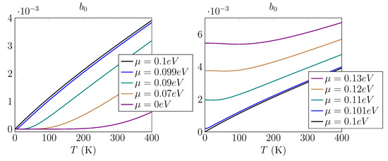
Figure 1. The functions $b_0$ for $a=100$ nm, $m=0.1$ eV, and different values of chemical potential $\mu$. For $\mu <m$, the function $b_0\sim 0$ for low temperatures; for $\mu =m$, it is linear, and, for $\mu >m$, it starts from constant values in agreement with Equation (19).

In the first case (19a) with $\mu >m$, the expansion $b_0$ over T starts from the constant term (see Figure 1, right panel), and we obtain the following non-zero coefficients

$$\begin{array}{ccc}\hfill A_3^{\mathsf{tm}}& =& \frac{1}{3},A_3^{\mathsf{te}}=-1,\hfill \\ \hfill A_5^{\mathsf{tm}}& =& \frac{{\alpha }^{″}(0)}{6a^2\alpha (0)}+\frac{2}{3{\eta }_{\mathsf{gr}}{b}_0}-\frac{3}{{\eta }_{\mathsf{gr}}^2{b}_0^2}-\frac{2}{15},A_5^{\mathsf{te}}=-\frac{{\alpha }^{″}(0)}{2a^2\alpha (0)}-\frac{2}{3{\eta }_{\mathsf{gr}}{b}_0}-\frac{1}{3{\eta }_{\mathsf{gr}}^2{b}_0^2}-\frac{2}{3},\hfill \\ \hfill B_4^{\mathsf{tm}}& =& -\frac{1}{{\eta }_{\mathsf{gr}}{b}_0},B_6^{\mathsf{tm}}=-\frac{{\alpha }^{″}(0)}{2a^2\alpha (0){\eta }_{\mathsf{gr}}{b}_0}+\frac{b_2-2}{{\eta }_{\mathsf{gr}}^2{b}_0^2}+\frac{2}{{\eta }_{\mathsf{gr}}^3{b}_0^3}.\hfill \end{array}$$

(20)

The main contribution to the $b_0$ comes from the first term of expansion in Equation (19a):

$$b_0=\frac{4a}{\pi }\frac{{\mu }^2-m^2}{\mu }.$$

(21)

In the last case (19c) with $\mu <m$, the $b_0$ is exponentially small (see Figure 1, left panel), and we set it at zero, and the conductivities are expanded as the following:

$$\frac{{\eta }_{\mathsf{x}}}{{\eta }_{\mathsf{gr}}}=z(b_2+z^2{b}_4+\dots ),$$

(22)

and the firsts non-zero coefficients read

$$A_5^{\mathsf{tm}}=\frac{1}{15}{\eta }_{\mathsf{gr}}{b}_2({\eta }_{\mathsf{gr}}{b}_2+2),A_5^{\mathsf{te}}=2{\eta }_{\mathsf{gr}}{b}_2,B_4^{\mathsf{te}}=-{\eta }_{\mathsf{gr}}{b}_2.$$

(23)

For the specific case (19b), when $\mu =m$, we consider the main contribution for $T\to 0$ and can set $b_0=0$, as in the case (19c). Therefore, for all cases, we have the following expansion up to $T^5$:

$$\begin{array}{ccc}\hfill \frac{\Delta \mathcal{F}}{{\mathcal{E}}_{\mathsf{CP}}^{\infty }}& =& -\frac{16{\pi }^4}{135}{(aT)}^4+\frac{8{\pi }^2{\zeta }_R(3)\mu }{a{\eta }_{\mathsf{gr}}({\mu }^2-m^2)}{(aT)}^5+\dots ,(\mu >m,T\ll \mu -m),\hfill \\ \hfill \frac{\Delta \mathcal{F}}{{\mathcal{E}}_{\mathsf{CP}}^{\infty }}& =& \frac{128{\eta }_{\mathsf{gr}}{\zeta }_R(5)}{3am}{(aT)}^5+\dots ,(\mu =m,T\ll m),\hfill \\ \hfill \frac{\Delta \mathcal{F}}{{\mathcal{E}}_{\mathsf{CP}}^{\infty }}& =& \frac{128{\eta }_{\mathsf{gr}}{\zeta }_R(5)}{3am}{(aT)}^5+\dots ,(\mu <m,T\ll m-\mu ).\hfill \end{array}$$

(24)

2.2. Expansion of the ${\mathcal{F}}^0$

The zero term reads

$$\frac{{\mathcal{F}}_{\mathsf{tm}|\mathsf{te}}^0}{{\mathcal{E}}_{\mathsf{CP}}^{\infty }}=\frac{4}{3}{\int }_0^{\infty }{z}^3{e}^{-2z}dz{\int }_0^{1}dx\frac{\alpha (\frac{zx}{a})}{\alpha (0)}\left\{\left.\frac{2-x^2}{1+\frac{x}{{\eta }^{\mathsf{tm}}}}\right|\frac{x^2}{1+\frac{1}{x{\eta }^{\mathsf{te}}}}\right\}.$$

(25)

The conductivities (6) depend on the temperature, and $\Delta {\eta }_{\mathsf{x}}$ have the following low-temperature expansions [23]

I. $\mu >m,T\ll \mu -m$

$$\frac{\Delta {\eta }_{\mathsf{x}}}{{\eta }_{\mathsf{gr}}}={\int }_m^{\mu }{f}_{\mathsf{x}}(y)dy+\frac{{\pi }^2}{6}{T}^2{f}_{\mathsf{x}}^{\prime }(\mu )+\frac{7{\pi }^4}{360}{T}^4{f}_{\mathsf{x}}^{‴}(\mu )+O(e^{-\frac{\mu -m}{T}}).$$

(26a)

II. $\mu =m,T\ll m$

$$\frac{\Delta {\eta }_{\mathsf{x}}}{{\eta }_{\mathsf{gr}}}=Tln2f_{\mathsf{x}}(m)+\frac{{\pi }^2}{12}{T}^2{f}_{\mathsf{x}}^{\prime }(m)+\frac{3}{4}{\zeta }_R(3)T^3{f}_{\mathsf{x}}^{″}(m)+\frac{7{\pi }^4}{720}{T}^4{f}_{\mathsf{x}}^{‴}(m)+O(e^{-\frac{m}{T}}).$$

(26b)

III. $\mu <m,T\ll m-\mu$

$$\frac{\Delta {\eta }_{\mathsf{x}}}{{\eta }_{\mathsf{gr}}}=O(e^{-\frac{m-\mu }{T}}).$$

(26c)

Taking these expansions into account, we obtain the following low-temperature corrections to zero term

$$\begin{array}{ccc}\hfill \frac{\Delta {\mathcal{F}}_{\mathsf{x}}^0}{{\mathcal{E}}_{\mathsf{CP}}^{\infty }}& =& {(aT)}^2{G}_{\mathsf{x}},(\mu >m,T\ll \mu -m),\hfill \\ \hfill \frac{\Delta {\mathcal{F}}_{\mathsf{x}}^0}{{\mathcal{E}}_{\mathsf{CP}}^{\infty }}& =& (aT)H_{\mathsf{x}},(\mu =m,T\ll m),\hfill \\ \hfill \frac{\Delta {\mathcal{F}}_{\mathsf{x}}^0}{{\mathcal{E}}_{\mathsf{CP}}^{\infty }}& =& 0,(\mu <m,T\ll \mu -m),\hfill \end{array}$$

(27)

where

$$\begin{array}{ccc}\hfill G_{\mathsf{tm}|\mathsf{te}}& =& \frac{2{\pi }^2}{9a^2}{\int }_0^{\infty }{z}^3{e}^{-2z}dz{\int }_0^{1}dx\frac{\alpha (\frac{zx}{a})}{\alpha (0)}\left\{\left.\frac{(2-x^2)x{f}_{\mathsf{tm}}^{\prime }(\mu )}{{(x+{\eta }_{\mathsf{tm}}^0+{\Delta }_0{\eta }_{\mathsf{tm}})}^2}\right|\frac{x^3{f}_{\mathsf{te}}^{\prime }(\mu )}{{(1+x\left({\eta }_{\mathsf{te}}^0+{\Delta }_0{\eta }_{\mathsf{te}}\right))}^2}\right\},\hfill \\ \hfill H_{\mathsf{tm}|\mathsf{te}}& =& \frac{4ln2}{3a}{\int }_0^{\infty }{z}^3{e}^{-2z}dz{\int }_0^{1}dx\frac{\alpha (\frac{zx}{a})}{\alpha (0)}\left\{\left.\frac{(2-x^2)x{f}_{\mathsf{tm}}(m)}{{(x+{\eta }_{\mathsf{tm}}^0)}^2}\right|\frac{x^3{f}_{\mathsf{te}}(m)}{{(1+x{\eta }_{\mathsf{te}}^0)}^2}\right\}.\hfill \end{array}$$

(28)

The functions $f_{\mathsf{x}}$ are given by Equation (6) and

$${\Delta }_0{\eta }_{\mathsf{x}}={\eta }_{\mathsf{gr}}{\int }_m^{\mu }{f}_{\mathsf{x}}(y)dy.$$

(29)

Therefore, taking into account (24), we obtain the low-temperature expansion of the free energy

$$\begin{array}{ccc}\hfill \frac{{\Delta }_T\mathcal{F}}{{\mathcal{E}}_{\mathsf{CP}}^{\infty }}& =& {(aT)}^2(G_{\mathsf{tm}}+G_{\mathsf{te}}),(\mu >m,T\ll \mu -m),\hfill \end{array}$$

(30a)

$$\begin{array}{ccc}\hfill \frac{{\Delta }_T\mathcal{F}}{{\mathcal{E}}_{\mathsf{CP}}^{\infty }}& =& (aT)(H_{\mathsf{tm}}+H_{\mathsf{te}}),(\mu =m,T\ll m),\hfill \end{array}$$

(30b)

$$\begin{array}{ccc}\hfill \frac{{\Delta }_T\mathcal{F}}{{\mathcal{E}}_{\mathsf{CP}}^{\infty }}& =& \frac{128{\eta }_{\mathsf{gr}}{\zeta }_R(5)}{3am}{(aT)}^5+\dots (\mu <m,T\ll m-\mu ).\hfill \end{array}$$

(30c)

3. Numerical Evaluations

We evaluated numerically the total temperature correction (5) by using the expression for the free energy in the form of Matsubara sum. We considered the Hydrogen atom at distance $a=100$ nm from the graphene sheet. The polarizability of the Hydrogen atom in the single oscillator approximation may be found in Ref. [8], for example. The graphene conductivities are given by Equations (6). We used the Fermi velocity $v_F=1/300$ and the mass gap $m=0.1$ eV. To visualize the dynamic of $\mu$ dependence, we made calculations for the value of $\mu$ close to $m=0.1$ eV. The free energy is normalized to the ${\mathcal{E}}_{\mathsf{CP}}^{\infty }=-3\alpha (0)/8\pi a^4$—the CPenergy for an ideal plane/atom at large distance a.

The zero-temperature free energy, ${\mathcal{F}}^{T=0}$, depends on the chemical potential $\mu$, and this dependence is shown in Figure 2. For $\mu \le m$, it has the constant value, and it grows up starting with mass gap $\mu >m$.

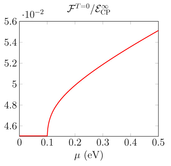
Figure 2. The zero temperature free energy, ${\mathcal{F}}^{T=0}$, as a function of chemical potential $\mu$.

We proceed now to the consideration of the temperature correction, ${\Delta }_T\mathcal{F}$ to the free energy. First of all, let us consider the functions $G_{\mathsf{x}}$, which define low temperature expansion for $\mu >m$ case (30a). They are plotted in Figure 3. We observe that they are negative, and contribution from the TE mode is 100 times smaller.

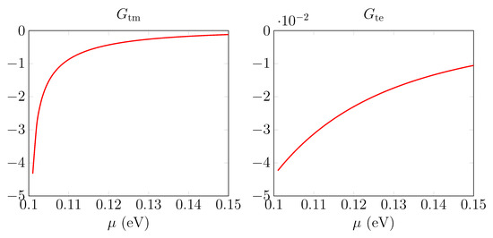
Figure 3. The functions $G_{\mathsf{x}}$ (30a) for different values of the chemical potential $\mu >m$.

One comment is in order. Because $G_{\mathsf{x}}<0$, then the temperature correction ${\Delta }_T\mathcal{F}>0$ close to the $T=0$. At the same time, in Refs. [7,24], the positive value of correction was observed. The disagreement is connected with that in which we use distance $a=100$ nm for numerical evaluations, which is out of distances considered in Refs. [7,24].

The numerical evaluation of $H_{\mathsf{x}}(a)$ for $a=100$ nm gives the following values $H_{\mathsf{tm}}=3\times {10}^6$ and $H_{\mathsf{te}}=0.18$. Again, the main contribution comes from TM mode. The value of $H_{\mathsf{tm}}$ strongly depends on the value of the Fermi velocity. For $v_F\to 0$, the $H_{\mathsf{tm}}\to \infty$.

The temperature contribution for $\mu \ge m$ is shown in Figure 4. We observe that, for low temperatures, the free energy has the form of parabola, ∼$G_{\mathsf{tm}}{(aT)}^2$, in agreement with (30) with negative parameter $G_{\mathsf{tm}}$ (see Figure 3).

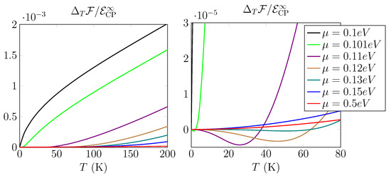
Figure 4. The temperature contribution to the free energy in the different intervals of temperatures and $\mu \ge m$.

The closer $\mu >m$ to m, the smaller domain of temperature T where this approximation is valid, and the greater value of the parameter of parabola $G_{\mathsf{tm}}$, in agreement with Figure 3. If $\mu =m$, this domain becomes zero, and the free energy drastically changes its form. If $\mu \to 0$, the part of the curve which is out of this domain (the vertical part of the green curve, for example) goes to free energy for this very special position with $\mu =m$ (black curve). Therefore, for any infinitely small difference $\mu -m\ne 0$, the derivative of free energy with respect temperature T is zero for $T=0$, and the Nernst theorem is valid. The experimental realization of the exact equality $\mu =m$ cannot be realized, and we conclude that the Nernst theorem is valid for this system.

The temperature contribution for $\mu \le m$ is shown in Figure 5. We observe the completely different dependence of the energy on the $\mu$.

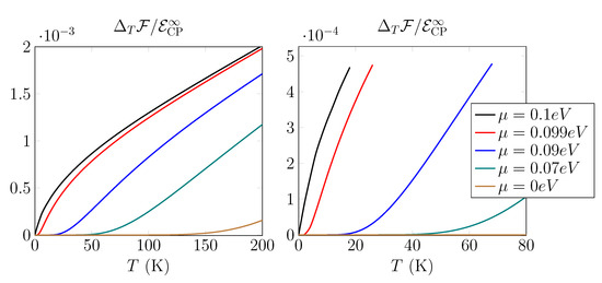
Figure 5. The temperature contribution to the free energy in the different intervals of temperatures and $\mu \le m$.

For zero chemical potential (brown curve), the temperature correction is, in fact, zero for the large domain of temperatures. The closer $\mu$ to m, the smaller domain in which temperature correction is zero. According to (30b),

$$\frac{{\Delta }_T\mathcal{F}}{{\mathcal{E}}_{\mathsf{CP}}^{\infty }}=\frac{128{\eta }_{\mathsf{gr}}{\zeta }_R(5)}{3am}{(aT)}^5={10}^{-24}{T}^5(K),$$

(31)

in this domain.

Figure 6 shows the temperature contribution to the free energy as a function of chemical potential. The function has a very sharp form with the maximum for $\mu =m$ with a different slope at the left and the right of this point.

Figure 6. The temperature contribution to the free energy as a function of the chemical potential for distance between Hydrogen atom and graphene $a=100$ nm.

The point $\mu =m$ looks like a phase transition point between different regimes from ${\Delta }_T\mathcal{F}\sim T^4$ to ${\Delta }_T\mathcal{F}\sim T^2$. In fact, it is an unstable point—infinitely small deviation $\mu$ from m changes regime.

From Figure 4 and Figure 5 and relations (30), we observe the different signs of the entropy, S, for $\mu <m$ and $\mu >m$. The entropy is the negative derivative of the free energy with respect of temperature. Therefore, $S^{\mu <m}<0$ (see Figure 5), and $S^{\mu >m}>0$ (see Figure 4). In both cases, the Nernst theorem is valid, $S_{T\to 0}\to 0$. The negative entropy of the dispersion forces has already been observed in Refs. [19,33] for plain and spherical configurations in the framework of plasma model and was also discussed recently in Ref. [34].

The domains of temperatures where the low-temperature expansions (30) over dimensionless parameter $(aT)\ll 1$ are valid depend on the chemical potential $\mu$, mass gap m, and the distance a between an atom and plain. Let us make some numerical estimations. The mass gap $m=0.1$ eV corresponds to the temperature $T_m=1160$ K. Therefore, the restriction $T\ll |\mu -m|$ in Equations (30a) and (30c) plays the role for $|\mu -m|<0.1$ eV, in agreement with Figure 4 and Figure 5. The restriction in the second case (30b) plays the role if $T\ll m<0.1$ eV. The more strong limitation appears due to the huge value of parameter $H_{\mathsf{tm}}\sim {10}^6$ (for $a=100$ nm): $T\ll {(H_{\mathsf{tm}}a)}^{-1}=0.14$ K for $a=100$ nm. It means that, in this case, there is no domain of temperatures where this case is valid, according to above discussion. The restriction $(aT)\ll 1$ is important starting from $a=10$μm. In this case, the effective temperature $T_a=1/a=1438$ K.

4. Conclusions

We considered the low-temperature correction to the Casimir-Polder free energy for atom/graphene system by using the Poisson representation of the free energy, which is more suitable for low-temperature analysis. The analysis is naturally broken into three different regions, (i) $\mu >m$, (ii) $\mu =m$, and (iii) $\mu <m$, for chemical potential. This division is the consequence of the same regions for the conductivity of graphene (see Equation (26). The conductivities have completely different expansion in these regions. It starts from the constant in the first region, linear on the temperature in the second one, and exponentially small in the third region.

The free energy may be divided into the two parts (3). The first one, ${\mathcal{F}}^0$, has the form of the free energy at zero temperature but with $\mu ,m$, and T dependence via the conductivity dependence on these parameters. The main contribution in the low-temperature expansion in the first (i) and second (ii) regimes comes from this first term, and it is quadratic and linear on the temperature, correspondingly (see Equation (30). In the third (iii) regime, the main contribution $\sim T^5$ comes from the rest part $\Delta \mathcal{F}$.

References

- Casimir, H.B.G. On the attraction between two perfectly conducting plates. Kon. Ned. Akad. Wetensch. Proc. 1948, 51, 793–795. [Google Scholar]
- Casimir, H.B.G.; Polder, D. The influence of retardation on the London-van der Waals forces. Phys. Rev. 1948, 73, 360–372. [Google Scholar] [CrossRef]
- Parsegian, A.V. Van der Waals Forces. A Handbook for Biologists, Chemists, Engineers, and Physicists; Cambridge University Press: Cambridge, UK, 2006; p. 380. [Google Scholar]
- Bordag, M.; Klimchitskaya, G.L.; Mohideen, U.; Mostepanenko, V.M. Advances in the Casimir Effect; Cambridge University Press: Cambridge, UK, 2009; pp. 1–768. [Google Scholar] [CrossRef]
- Bondarev, I.V.; Lambin, P. Van der Waals coupling in atomically doped carbon nanotubes. Phys. Rev. B 2005, 72, 35451. [Google Scholar] [CrossRef]
- Blagov, E.V.; Klimchitskaya, G.L.; Mostepanenko, V.M. Van der Waals interaction between a microparticle and a single-wall carbon nanotube. Phys. Rev. B 2007, 75, 235413. [Google Scholar] [CrossRef]
- Klimchitskaya, G.L.; Mostepanenko, V.M. Casimir and Casimir-Polder Forces in Graphene Systems: Quantum Field Theoretical Description and Thermodynamics. Universe 2020, 6, 150. [Google Scholar] [CrossRef]
- Khusnutdinov, N.; Kashapov, R.; Woods, L.M. Casimir-Polder effect for a stack of conductive planes. Phys. Rev. A 2016, 94, 12513. [Google Scholar] [CrossRef]
- Khusnutdinov, N.; Woods, L.M. Casimir Effects in 2D Dirac Materials (Mini-review). JETP Lett. 2019, 110, 1–10. [Google Scholar] [CrossRef]
- Babb, J.F. Long-range atom-surface interactions for cold atoms. J. Phys. Conf. Ser. 2005, 19, 1–9. [Google Scholar] [CrossRef]
- Marachevsky, V.N.; Pis’mak, Y.M. Casimir-Polder effect for a plane with Chern-Simons interaction. Phys. Rev. D 2010, 81, 65005. [Google Scholar] [CrossRef]
- Shajesh, K.V.; Schaden, M. Repulsive long-range forces between anisotropic atoms and dielectrics. Phys. Rev. A 2012, 85, 012523. [Google Scholar] [CrossRef]
- Thiyam, P.; Parashar, P.; Shajesh, K.V.; Persson, C.; Schaden, M.; Brevik, I.; Parsons, D.F.; Milton, K.A.; Malyi, O.I.; Boström, M. Anisotropic contribution to the van der Waals and the Casimir-Polder energies for CO2 and CH4 molecules near surfaces and thin films. Phys. Rev. A 2015, 92, 052704. [Google Scholar] [CrossRef]
- Antezza, M.; Fialkovsky, I.; Khusnutdinov, N. Casimir-Polder force and torque for anisotropic molecules close to conducting planes and their effect on CO2. Phys. Rev. B 2020, 102, 195422. [Google Scholar] [CrossRef]
- Obrecht, J.M.; Wild, R.J.; Antezza, M.; Pitaevskii, L.P.; Stringari, S.; Cornell, E.A. Measurement of the Temperature Dependence of the Casimir-Polder Force. Phys. Rev. Lett. 2007, 98, 063201. [Google Scholar] [CrossRef] [PubMed]
- Laliotis, A.; de Silans, T.P.; Maurin, I.; Ducloy, M.; Bloch, D. Casimir-Polder interactions in the presence of thermally excited surface modes. Nat. Commun. 2014, 5. [Google Scholar] [CrossRef]
- Wylie, J.M.; Sipe, J.E. Quantum electrodynamics near an interface. II. Phys. Rev. A 1985, 32, 2030–2043. [Google Scholar] [CrossRef] [PubMed]
- Buhmann, S.; Welsch, D. Dispersion forces in macroscopic quantum electrodynamics. Prog. Quantum Electron. 2007, 31, 51–130. [Google Scholar] [CrossRef]
- Bezerra, V.B.; Klimchitskaya, G.L.; Mostepanenko, V.M.; Romero, C. Lifshitz theory of atom-wall interaction with applications to quantum reflection. Phys. Rev. A 2008, 78, 042901. [Google Scholar] [CrossRef]
- Chaichian, M.; Klimchitskaya, G.L.; Mostepanenko, V.M.; Tureanu, A. Thermal Casimir-Polder interaction of different atoms with graphene. Phys. Rev. A 2012, 86, 12515. [Google Scholar] [CrossRef]
- Bordag, M. Low Temperature Expansion in the Lifshitz Formula. Adv. Math. Phys. 2014, 2014, 1–34. [Google Scholar] [CrossRef]
- Khusnutdinov, N.; Kashapov, R.; Woods, L.M. Thermal Casimir and Casimir–Polder interactions in N parallel 2D Dirac materials. 2D Mater. 2018, 5, 35032. [Google Scholar] [CrossRef]
- Khusnutdinov, N.; Emelianova, N. Low-temperature expansion of the Casimir-Polder free energy for an atom interacting with a conductive plane. Int. J. Mod. Phys. A 2019, 34, 1950008. [Google Scholar] [CrossRef]
- Klimchitskaya, G.L.; Mostepanenko, V.M. Nernst heat theorem for an atom interacting with graphene: Dirac model with nonzero energy gap and chemical potential. Phys. Rev. D 2020, 101, 116003. [Google Scholar] [CrossRef]
- Klimchitskaya, G.L.; Mostepanenko, V.M. Quantum field theoretical description of the Casimir effect between two real graphene sheets and thermodynamics. Phys. Rev. D 2020, 102, 016006. [Google Scholar] [CrossRef]
- Bordag, M.; Fialkovsky, I.V.; Gitman, D.M.; Vassilevich, D.V. Casimir interaction between a perfect conductor and graphene described by the Dirac model. Phys. Rev. B 2009, 80, 245406. [Google Scholar] [CrossRef]
- Fialkovsky, I.V.; Marachevsky, V.N.; Vassilevich, D.V. Finite-temperature Casimir effect for graphene. Phys. Rev. B 2011, 84, 35446. [Google Scholar] [CrossRef]
- Bordag, M.; Klimchitskaya, G.L.; Mostepanenko, V.M.; Petrov, V.M. Quantum field theoretical description for the reflectivity of graphene. Phys. Rev. D 2015, 91, 045037. [Google Scholar] [CrossRef]
- Bordag, M.; Fialkovskiy, I.; Vassilevich, D. Enhanced Casimir effect for doped graphene. Phys. Rev. B 2016, 93, 075414, Erratum in Phys. Rev. B 2017, 95, 119905. doi:10.1103/physrevb.95.119905. [Google Scholar] [CrossRef]
- Falkovsky, L.A.; Varlamov, A.A. Space-time dispersion of graphene conductivity. Eur. Phys. J. B 2007, 56, 281–284. [Google Scholar] [CrossRef]
- Gusynin, V.P.; Sharapov, S.G.; Carbotte, J.P. Magneto-optical conductivity in Graphene. J. Phys. Condens. Matter 2007, 19, 26222. [Google Scholar] [CrossRef]
- Fedoryuk, M.V. The Saddle-Point Method; Nauka: Moscow, Russia, 1977. (In Russian) [Google Scholar]
- Khusnutdinov, N.R. The thermal Casimir–Polder interaction of an atom with a spherical plasma shell. J. Phys. A Math. Theor. 2012, 45, 265301. [Google Scholar] [CrossRef]
- Li, Y.; Milton, K.; Parashar, P.; Hong, L. Negativity of the Casimir Self-Entropy in Spherical Geometries. Entropy 2021, 23, 214. [Google Scholar] [CrossRef] [PubMed]
Publisher’s Note: MDPI stays neutral with regard to jurisdictional claims in published maps and institutional affiliations. |
© 2021 by the authors. Licensee MDPI, Basel, Switzerland. This article is an open access article distributed under the terms and conditions of the Creative Commons Attribution (CC BY) license (http://creativecommons.org/licenses/by/4.0/).