Generalised Asymptotic Solutions for the Inflaton in the Oscillatory Phase of Reheating

Abstract

We determine generalised asymptotic solutions for the inflaton field, the Hubble parameter, and the equation-of-state parameter valid during the oscillatory phase of reheating for potentials that close to their global minima behave as even monomial potentials. For the quadratic potential, we derive a generalised asymptotic expansion for the inflaton with respect to the scale set by inverse powers of the cosmic time. For the quartic potential, we derive an explicit, two-term generalised asymptotic solution in terms of Jacobi elliptic functions, with a scale set by inverse powers of the square root of the cosmic time. In the general case, we find similar two-term solutions where the leading order term is defined implicitly in terms of the Gauss hypergeometric function. The relation between the leading terms of the instantaneous equation-of-state parameter and different averaged values is discussed in the general case. Finally, we discuss the physical significance of the generalised asymptotic solutions in the oscillatory regime and their matching to the appropriate solutions in the thermalization regime.

1. Introduction

The reheating period in inflationary cosmology is a transition period connecting the end of inflation to the radiation-dominated era [1,2,3,4,5,6,7,8]. During reheating, the energy of the inflaton field $\mathsf{\Phi }$ transforms into relativistic particles. A basic model for the inflaton decay is given by the system of Equations [1,9,10]

$$\ddot{\mathsf{\Phi }}+(3H+\mathsf{\Gamma })\dot{\mathsf{\Phi }}+V^{\prime }\left(\mathsf{\Phi }\right)=0,$$

(1)

$${\dot{\rho }}_{\gamma }=-4{\rho }_{\gamma }H+(1+w_{\mathsf{\Phi }})\mathsf{\Gamma }{\rho }_{\mathsf{\Phi }},$$

(2)

where dots denote derivatives with respect to the cosmic time t, and $V\left(\mathsf{\Phi }\right)$ is the inflaton potential. The inflaton pressure, energy density, and equation of state (eos) parameter are given, respectively, by

$$p_{\mathsf{\Phi }}=\frac{1}{2}{\dot{\mathsf{\Phi }}}^2-V\left(\mathsf{\Phi }\right),$$

(3)

$${\rho }_{\mathsf{\Phi }}=\frac{1}{2}{\dot{\mathsf{\Phi }}}^2+V\left(\mathsf{\Phi }\right),$$

(4)

$$w_{\mathsf{\Phi }}=p_{\mathsf{\Phi }}/{\rho }_{\mathsf{\Phi }},$$

(5)

$\mathsf{\Gamma }$ is the total inflaton decay rate, ${\rho }_{\gamma }$ is energy density of the radiation, and the Hubble parameter H satisfies the Friedmann–Lemaître Equation

$$H^2=\frac{1}{3{\mathrm{M}}_{\mathrm{Pl}}^2}({\rho }_{\mathsf{\Phi }}+{\rho }_{\gamma }),$$

(6)

with ${\mathrm{M}}_{\mathrm{Pl}}=2.435\times {10}^{18} \mathrm{GeV}$ being the reduced Planck mass.

The model (1)–(2) represents reheating in terms of an effective fluid with total pressure $p=p_{\mathsf{\Phi }}+p_{\gamma }$ and density $\rho ={\rho }_{\mathsf{\Phi }}+{\rho }_{\gamma }$. The radiation eos $p_{\gamma }={\rho }_{\gamma }/3$ leads to an eos parameter during reheating given by [10]

$$w_{\mathrm{re}}=\frac{p}{\rho }=\frac{\frac{1}{2}{\dot{\mathsf{\Phi }}}^2-V\left(\mathsf{\Phi }\right)+\frac{1}{3}{\rho }_{\gamma }}{\frac{1}{2}{\dot{\mathsf{\Phi }}}^2+V\left(\mathsf{\Phi }\right)+{\rho }_{\gamma }}.$$

(7)

The first phase of reheating can be described as an oscillatory phase around the true minimum of the inflaton potential, wherein the inflaton is not yet effectively coupled to the radiation fields, and the friction term $\mathsf{\Gamma }\dot{\mathsf{\Phi }}$ in Equation (1) can be neglected. During this period, Equations (1) and (6) reduce to

$$\ddot{\mathsf{\Phi }}+3H\dot{\mathsf{\Phi }}+V^{\prime }\left(\mathsf{\Phi }\right)=0,$$

(8)

$$H^2=\frac{1}{3{\mathrm{M}}_{\mathrm{Pl}}^2}\left(\frac{1}{2}{\dot{\mathsf{\Phi }}}^2+V\left(\mathsf{\Phi }\right)\right).$$

(9)

Conversely, in the last phase of reheating, the term $3H\dot{\mathsf{\Phi }}$ can be neglected with respect to $\mathsf{\Gamma }\dot{\mathsf{\Phi }}$ in (1), leading to the simple equation

$$\ddot{\mathsf{\Phi }}+\mathsf{\Gamma }\dot{\mathsf{\Phi }}+V^{\prime }\left(\mathsf{\Phi }\right)=0.$$

(10)

During the oscillatory period, where ${\rho }_{\gamma }\ll {\rho }_{\mathsf{\Phi }}$, $w_{\mathrm{re}}$ reduces to $w_{\mathsf{\Phi }}$, whereas, at the end of reheating, $\rho \sim {\rho }_{\gamma }$ and $w_{\mathrm{re}}$ tends to $1/3$, i.e., to the onset of the radiation era.

The aim of this paper is to determine generalised asymptotic solutions for the inflaton field $\mathsf{\Phi }\left(t\right)$ and derived quantities valid during the oscillatory phase of reheating for potentials that close to their global minima behave as the even monomial potentials

$$V\left(\mathsf{\Phi }\right)=\frac{M^4}{p}{\left(\frac{\mathsf{\Phi }}{{\mathrm{M}}_{\mathrm{Pl}}}\right)}^{2p},(p=1,2,\dots ).$$

(11)

Recently [8], it has been claimed that the origin of dark matter may reside in the process of reheating with potentials of the form (11) with $p>1$. We also mention that asymptotic solutions similar to those derived in this paper have been recently used to study the pre-inflationary (kinetic) and inflationary stages of inflaton models [11,12].

Turner [9], Mukhanov [5], and Rendall [13] emphasised that, during the oscillatory phase, the model is approximated in some averaged sense by a perfect fluid with a linear equation of state.

Since these generalised asymptotic solutions will be formally valid as the cosmic time t tends to infinity, we raise the question of its physical relevance in comparison with the exact solutions of the full Equations (1), (2) and (6), because the power-law-damped oscillatory approximation will certainly break down when $H\sim \mathsf{\Gamma }$ and ${\rho }_{\gamma }\gtrsim {\rho }_{\mathsf{\Phi }}$, and the oscillations become exponentially damped.

However, typical values of the parameters for, e.g., the nondegenerate case $p=1$, are $M=3\times {10}^{-3}{\mathrm{M}}_{\mathrm{Pl}}$ and $\mathsf{\Gamma }=1.375\times {10}^9$ GeV, and order-of-magnitude estimates and numerical calculations confirm that there is a large time interval (several e-folds) in which the asymptotic solutions in the oscillatory phase will be valid (see, for example, Figure 13 in Ref. [10]).

If we write

$$\mathsf{\Phi }\left(t\right)=\sqrt{\frac{2}{3}}{\mathrm{M}}_{\mathrm{Pl}}\phi \left(\tau \right),$$

(12)

where

$$\tau =mt,$$

(13)

and

$$m=\sqrt{\frac{3}{p}}{\left(\frac{2}{3}\right)}^{p/2}\frac{M^2}{{\mathrm{M}}_{\mathrm{Pl}}},$$

(14)

and substitute Equations (9) and (11) into (8), we find that the system is equivalent to the single non-linear differential equation

$${\phi }^{″}\left(\tau \right)+{({\phi }^{\prime }{\left(\tau \right)}^2+\phi {\left(\tau \right)}^{2p})}^{1/2}{\phi }^{\prime }\left(\tau \right)+p\phi {\left(\tau \right)}^{2p-1}=0.$$

(15)

Likewise, the Hubble parameter can be written in terms of $\phi$ as

$$H\left(t\right)=\frac{m}{3}h\left(\tau \right),$$

(16)

where, for later convenience, we introduced the reduced Hubble parameter

$$h\left(\tau \right)={({\phi }^{\prime }{\left(\tau \right)}^2+\phi {\left(\tau \right)}^{2p})}^{1/2}.$$

(17)

Incidentally, by differentiation, the former equation and using (15), we find that

$$h^{\prime }\left(\tau \right)=-{\phi }^{\prime }{\left(\tau \right)}^2.$$

(18)

As usual, primes denote derivatives of $\phi$ with respect to its argument.

By introducing polar coordinates in the $(\phi ,{\phi }^{\prime })$ plane, Mukhanov [5] and Rendall [13] find the first two terms of the asymptotic expansion of the inflaton field for the quadratic potential corresponding to $p=1$ in Equation (11). (In fact, Equation (24) of Ref. [13] corrects a mistake in Equation (5.45) of Ref. [5].) For general values of p and using different averaging procedures, the authors arrive at a common constant leading term for the averaged value

$$\langle w_{\mathsf{\Phi }}\rangle \sim \frac{p-1}{p+1},(t\to \infty ),$$

(19)

i.e., to the above-mentioned averaged linear equation of state. Thus, $\langle w_{\mathsf{\Phi }}\rangle \sim 0$ for $p=1$ and $\langle w_{\mathsf{\Phi }}\rangle \sim 1/3$ for $p=2$, which correspond to a universe dominated by nonrelativistic matter and to a universe dominated by radiation, respectively. It was noted by Turner [9] that the amplitude of the inflaton oscillations decreases as ${\tau }^{1/p}$. However, for $p\ge 2$, we are not aware of any explicit results for the asymptotic form of the inflaton field.

In Section 2, we reconsider the nondegenerate harmonic potential discussed by Mukhanov [5] and Rendall [13]. First, we present a method to calculate a generalised asymptotic expansion for the inflaton field

$$\phi \left(\tau \right)\sim \sum _{n=1}^{\infty }\frac{{\phi }_n\left(\tau \right)}{{\tau }^n},(\tau \to \infty ),$$

(20)

where the coefficients ${\phi }_n$ are periodic (and therefore bounded) functions. To calculate these expansions we substitute the ansatz (20) into Equation (15) and solve recursively the system of differential equations for the ${\phi }_n$. The requisite that ${\phi }_n$ be bounded is implemented by imposing the cancellation of resonant terms in these equations. As a byproduct, we will show how to calculate asymptotic expansions for derived quantities like H and $w_{\mathsf{\Phi }}$. A formal proof of the existence of the generalised asymptotic expansion (20) is deferred to Appendix A.

A straightforward generalisation of the ansatz (20) does not work for potentials (11) with $p>1$ because the resonant terms cannot be systematically eliminated past a certain order. Therefore, we look for generalised asymptotic formulas with a finite number of terms [14]. In Section 3, we discuss separately the quartic potential. This is a particularly relevant potential because the corresponding oscillatory phase of reheating is radiation-dominated, and the universe would be radiation-dominated since the end of inflation with an ensuing reduction of the uncertainty on the period were the observable perturbations of the universe were produced [15].

We obtain explicit asymptotic formulas for the inflaton field and derived quantities in terms of Jacobi elliptic functions, which have appeared recently in perturbative approaches to inflationary cosmology due to its relation to Hill’s Equation (16). In Section 4, we give a general derivation valid for any value of p, where the leading term of the asymptotic formula for the inflaton field is defined implicitly in terms of Gauss’ hypergeometric function, whereas the second term can be given explicitly in terms of the first. We also obtain the leading term of the instantaneous eos parameter $w_{\mathsf{\Phi }}$ and show how different averaged values of $w_{\mathsf{\Phi }}$ coincide with the standard result (19).

In Section 5, we discuss the physical significance of the generalised asymptotic solutions in the oscillatory regime and their matching to the appropriate solutions in the thermalization regime. In particular, we provide values for the cosmic time that marks the end of the oscillatory regime and of the Hubble parameter at that time. (The latter turns out to be independent of the degree $2p$ of the potential close to its absolute minimum.) We also illustrate these results with a numerical calculation. The paper ends with some brief remarks on possible developments and applications of these generalised solutions.

2. The Harmonic Potential

In this section, we consider the nondegenerate harmonic potential discussed by Turner [9], Mukhanov [5], and Rendall [13], which corresponds to setting $p=1$ in Equation (11), and for which Equation (15) reduces to

$${\phi }^{″}\left(\tau \right)+{({\phi }^{\prime }{\left(\tau \right)}^2+\phi {\left(\tau \right)}^2)}^{1/2}{\phi }^{\prime }\left(\tau \right)+\phi \left(\tau \right)=0.$$

(21)

As we mentioned in the introduction, we look for a generalised asymptotic expansion of $\phi \left(\tau \right)$ with respect to the asymptotic sequence ${\tau }^{-n}$, $(n=1,2,3,\dots )$ (see Section 10.3 of [16]),

$$\phi \left(\tau \right)\sim \sum _{n=1}^{\infty }\frac{{\phi }_n\left(\tau \right)}{{\tau }^n},(\tau \to \infty )$$

(22)

where the ${\phi }_n\left(\tau \right)$ are periodic functions. Substituting Equation (22) into Equation (21) and arranging the result by inverse powers of $\tau$ (note that all the derivatives of the ${\phi }_n\left(\tau \right)$ will also be periodic and, therefore, bounded), we find an infinite system of differential equations for the ${\phi }_n\left(\tau \right)$. The first three, which are enough to show the pattern, are:

$${\phi }_1^{″}+{\phi }_1=0,$$

(23)

$${\phi }_2^{″}+{\phi }_2=(2-{({\left({\phi }_1^{\prime }\right)}^2+{\phi }_1^2)}^{1/2}){\phi }_1^{\prime },$$

(24)

$${\phi }_3^{″}+{\phi }_3=4{\phi }_2^{\prime }-2{\phi }_1-\frac{{\phi }_1^2{\phi }_2^{\prime }-2{\phi }_1{\left({\phi }_1^{\prime }\right)}^2+{\phi }_2{\phi }_1{\phi }_1^{\prime }+2{\left({\phi }_1^{\prime }\right)}^2{\phi }_2^{\prime }-{\phi }_1^3}{{({\left({\phi }_1^{\prime }\right)}^2+{\phi }_1^2)}^{1/2}}.$$

(25)

Equation (23) is a harmonic oscillator, whose general solution can be written as

$${\phi }_1\left(\tau \right)=bcos(\tau -{\tau }_0).$$

(26)

Substituting this solution into the right hand side of Equation (24), we find

$${\phi }_2^{″}+{\phi }_2=b(b-2)sin(\tau -{\tau }_0).$$

(27)

Note that since the natural frequency of the the homogeneous equation ${\phi }_2^{″}+{\phi }_2=0$ is $\omega =1$, the inhomogeneous term $sin(\tau -{\tau }_0)$ is resonant, as would be $cos(\tau -{\tau }_0)$. (Terms in $sin\left(\omega (\tau -{\tau }_0)\right)$ or $cos\left(\omega (\tau -{\tau }_0)\right)$ with $\omega \ne 1$ appearing below are not resonant.) Therefore, the solution for ${\phi }_2\left(\tau \right)$ would be unbounded unless we set $b=2$ ($b=0$ leads to a trivial solution for ${\phi }_1\left(\tau \right)$), and we have again a harmonic oscillator with general solution

$${\phi }_2\left(\tau \right)=ccos(\tau -{\tau }_0)+dsin(\tau -{\tau }_0).$$

(28)

Substituting this solution into the right-hand side of Equation (25) we find,

$${\phi }_3^{″}+{\phi }_3=\left(1+2d\right)cos(\tau -{\tau }_0)-cos\left(3(\tau -{\tau }_0)\right).$$

(29)

The first term in the right-hand side is again resonant, and the solution for ${\phi }_3\left(\tau \right)$ would be unbounded unless we set $d=-1/2$. The coefficient c remains free.

This recursive procedure can be easily programmed in a computer: at each stage, the function ${\phi }_n\left(\tau \right)$ is substituted into the right-hand side of the equation for ${\phi }_{n+1}\left(\tau \right)$ and resonant terms eliminated. It turns out that all the coefficients depend only on ${\tau }_0$ and c. The first four coefficients are:

$$\begin{array}{lll}{\phi }_1\left(\tau \right)\hfill & =& 2cos(\tau -{\tau }_0),\hfill \end{array}$$

(30)

$$\begin{array}{lll}{\phi }_2\left(\tau \right)\hfill & =& ccos(\tau -{\tau }_0)-\frac{1}{2}sin(\tau -{\tau }_0),\hfill \end{array}$$

(31)

$$\begin{array}{lll}{\phi }_3\left(\tau \right)\hfill & =& \frac{1}{16}\left(8c^2+9\right)cos(\tau -{\tau }_0)-\frac{c}{2}sin(\tau -{\tau }_0)+\frac{1}{8}cos\left(3(\tau -{\tau }_0)\right),\hfill \end{array}$$

(32)

$$\begin{array}{lll}{\phi }_4\left(\tau \right)\hfill & =& \frac{c}{32}\left(8c^2+27\right)cos(\tau -{\tau }_0)-\frac{1}{192}\left(72c^2+7\right)sin(\tau -{\tau }_0)\hfill \end{array}$$

(33)

$$\begin{array}{lll}& & +\frac{3c}{16}cos\left(3(\tau -{\tau }_0)\right)-\frac{5}{32}sin\left(3(\tau -{\tau }_0)\right).\hfill \end{array}$$

(34)

In light of these four coefficients one might conjecture the general form

$${\phi }_n\left(\tau \right)=\sum _{k=1,k\mathrm{odd}}^n{c}_{n,k}cos\left(k(\tau -{\tau }_0)\right)+d_{n,k}sin\left(k(\tau -{\tau }_0)\right),$$

(35)

with $d_{n,n}=0$ for n odd. (In fact, the most efficient way to calculate the expansion is to use this ansatz and to equate coefficients of the inverse powers of $\tau$.) A formal proof of the fact that Equation (35) is indeed true is deferred to Appendix A.

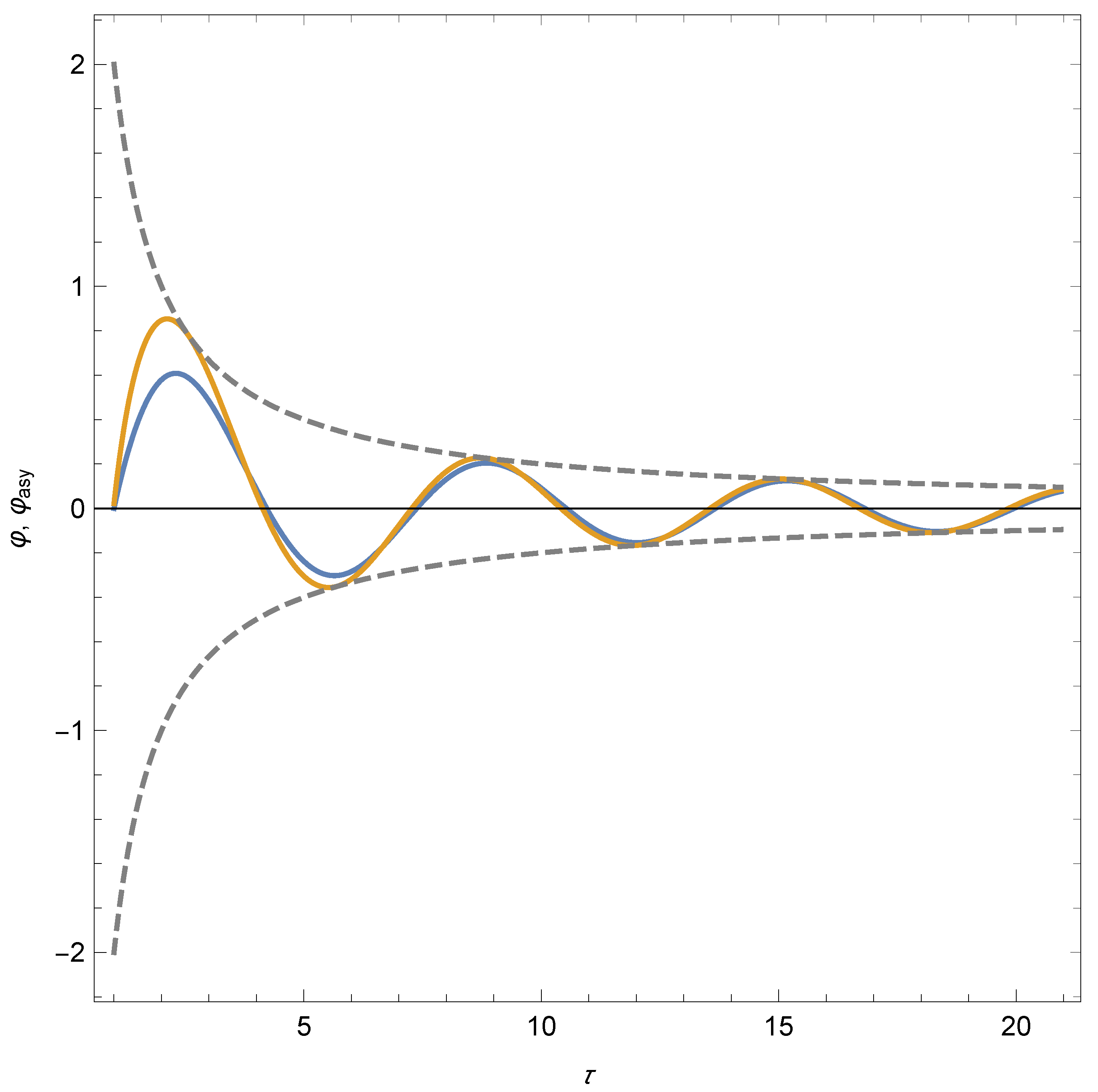
To illustrate the accuracy of this generalised asymptotic solution, in Figure 1 we plot the results of a numerical integration of the differential Equation (21) with initial conditions $\phi \left(1\right)=0$, ${\phi }^{\prime }\left(1\right)=1$, as well as the leading term of the asymptotic expansion (22). The numerical solution quickly tends to the asymptotic solution. The dashed lines are the envelopes $\pm 2/\tau$ that set the scale for the generalised asymptotic expansion (22). (The factor 2 is precisely the 2 in Equation (30) for ${\phi }_1\left(\tau \right)$.) Other initial conditions lead to similar plots and are not represented to avoid clutter in the figure.

As a consequence of the main expansion (22), we can calculate the corresponding expansion for the reduced Hubble parameter (17),

$$h\left(\tau \right)\sim \sum _{n=1}^{\infty }\frac{h_n\left(\tau \right)}{{\tau }^n},$$

(36)

whose first terms are

$$\begin{array}{lll}{h}_1\left(\tau \right)\hfill & =& 2,\hfill \end{array}$$

(37)

$$\begin{array}{lll}{h}_2\left(\tau \right)\hfill & =& c+sin\left(2(\tau -{\tau }_0)\right),\hfill \end{array}$$

(38)

$$\begin{array}{lll}{h}_3\left(\tau \right)\hfill & =& \frac{1}{4}(3+2c^2)+\frac{3}{2}cos\left(2(\tau -{\tau }_0)\right)+csin\left(2(\tau -{\tau }_0)\right).\hfill \end{array}$$

(39)

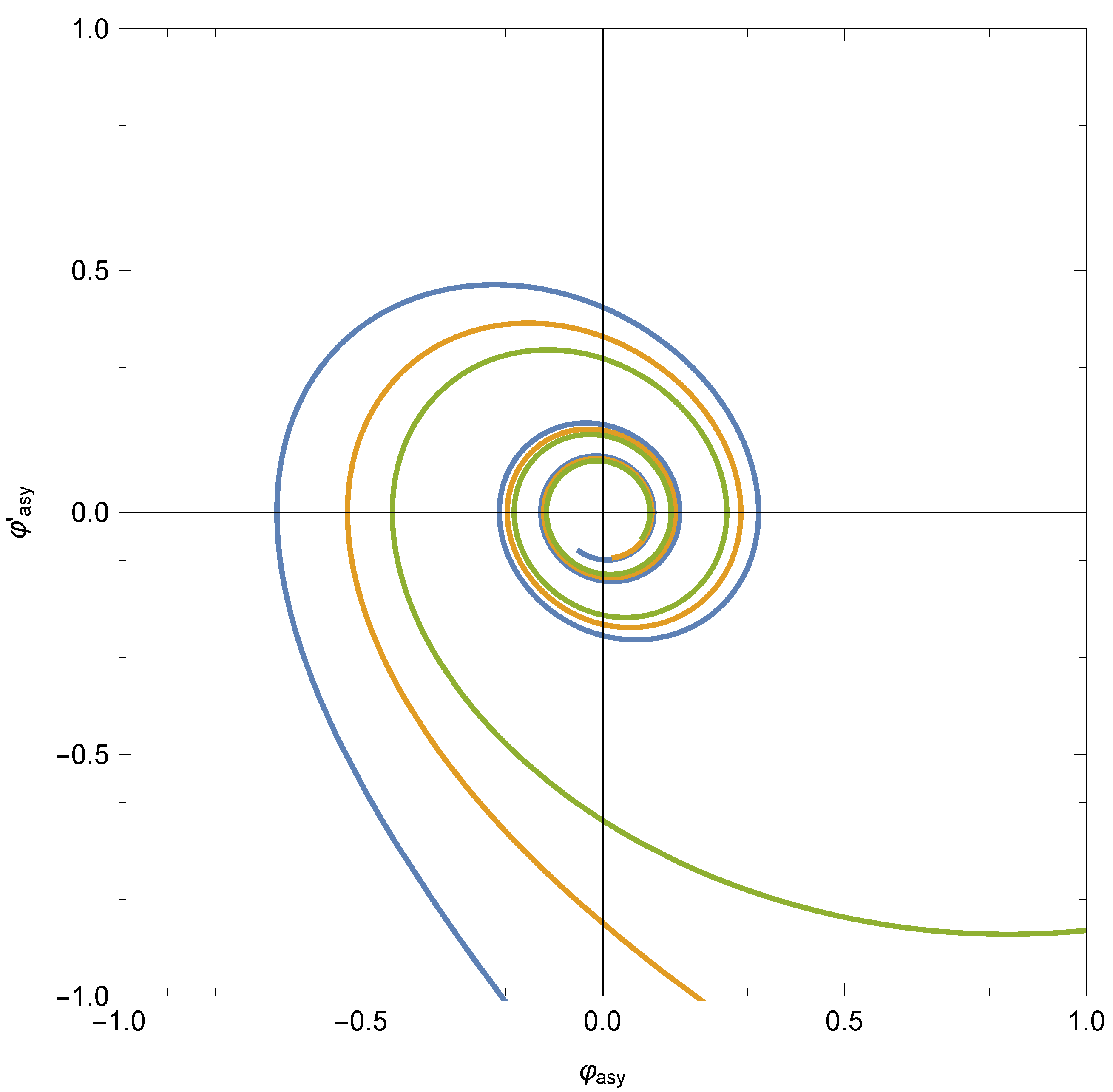
In Figure 2, we plot three typical asymptotic trajectories on the phase map of the differential Equation (21). Note that, for sufficiently large times, the approximation of the representative point to the origin is monotonic: in fact, for the quadratic potential, the distance of the representative point to the origin of the phase plane is simply the reduced Hubble constant $h\left(\tau \right)\sim 2/\tau$, as shown in Equation (37).

Using Equation (16), we find the expansion for the Hubble parameter

$$\begin{array}{l}\begin{array}{ll}H\left(t\right)\sim \hfill & \frac{2}{3t}+\frac{c+sin\left(2m(t-t_0)\right)}{3m{t}^2}\hfill \\ & +\frac{3+2c^2+4csin\left(2m(t-t_0)\right)+6cos\left(2m(t-t_0)\right)}{12m^2{t}^3}\cdots .\hfill \end{array}\hfill \end{array}$$

(40)

Here, m is the value of Equation (14) for $p=1$, i.e., $m=\sqrt{2}{M}^2/M_{\mathrm{Pl}}$, and ${\tau }_0=m{t}_0$. In this case, the inflaton potential reduces to

$$V\left(\mathsf{\Phi }\right)=\frac{1}{2}{m}^2{\mathsf{\Phi }}^2,$$

(41)

i.e., m is the $p=1$ inflaton mass. Likewise, using

$$w_{\mathsf{\Phi }}\left(t\right)=-1-\frac{2}{3}\frac{\dot{H}}{H^2},$$

(42)

we find the expansion for the equation of state parameter

$$\begin{array}{l}\begin{array}{ll}{w}_{\mathsf{\Phi }}\left(t\right)\sim \hfill & -cos\left(2m(t-t_0)\right)+\frac{3sin\left(2m(t-t_0)\right)+sin\left(4m(t-t_0)\right)}{2mt}\hfill \\ & +\frac{1}{16m^2{t}^2}(4+23cos\left(2m(t-t_0)\right)+12csin\left(2m(t-t_0)\right)\hfill \\ & +20cos\left(4m(t-t_0)\right)+4csin\left(4m(t-t_0)\right)+3cos\left(6m(t-t_0)\right))+\cdots .\hfill \end{array}\hfill \end{array}$$

(43)

Note that these first two terms of the complete asymptotic expansion for $w_{\mathsf{\Phi }}\left(t\right)$ are independent of c. Note also that the average of the leading term is trivially zero.

3. The Quartic Potential

In this section, we discuss the quartic potential, which corresponds to setting $p=2$ in Equation (15):

$${\phi }^{″}\left(\tau \right)+{({\phi }^{\prime }{\left(\tau \right)}^2+\phi {\left(\tau \right)}^4)}^{1/2}{\phi }^{\prime }\left(\tau \right)+2\phi {\left(\tau \right)}^3=0.$$

(44)

As was noted by Turner [9] and numerical calculations confirm, the solutions of this differential equation oscillate with a maximal amplitude that decreases as $1/{\tau }^{1/2}$. Therefore, one might try a generalised asymptotic solution similar to Equation (22) but with $\tau$ replaced by ${\tau }^{1/2}$ on the right-hand side of that equation. It turns out that resonant terms cannot be systematically eliminated at fourth order, and, as a consequence, there is an undetermined constant at third order. Therefore, we look for a two-term generalised asymptotic solution of the form

$$\phi \left(\tau \right)\sim \frac{{\phi }_1\left(\sigma \right)}{\sigma }+\frac{{\phi }_2\left(\sigma \right)}{{\sigma }^2}+o(1/{\sigma }^2),$$

(45)

where

$$\sigma ={\tau }^{1/2},$$

(46)

${\phi }_1\left(\sigma \right)$ and ${\phi }_2\left(\sigma \right)$ are periodic functions of $\sigma$. By substituting the ansatz (45) into Equation (44), we find the following equations for ${\phi }_1\left(\sigma \right)$ and ${\phi }_2\left(\sigma \right)$, which are the analogues of Equations (23) and (24):

$${\phi }_1^{″}+8{\left({\phi }_1\right)}^3=0,$$

(47)

$${\phi }_2^{″}+24{\left({\phi }_1\right)}^2{\phi }_2=(3-{({\left({\phi }_1^{\prime }\right)}^2+4{\phi }_1^4)}^{1/2}){\phi }_1^{\prime }.$$

(48)

Equation (47) for ${\phi }_1\left(\sigma \right)$ is a nonlinear differential equation whose solutions can be written in terms of the Jacobi elliptic function $\mathrm{sn}$ of modulus $-1$ [17]:

$${\phi }_1\left(\sigma \right)=b\mathrm{sn}\left(2b(\sigma -{\sigma }_0)\right|-1).$$

(49)

By substituting this solution into Equation (48), we find

$${\phi }_2^{″}+24{\left({\phi }_1\right)}^2{\phi }_2=(3-2b^2){\phi }_1^{\prime }.$$

(50)

Incidentally, that the square root ${({\left({\phi }_1^{\prime }\right)}^2+4{\phi }_1^4)}^{1/2}$ in Equation (48) reduces to the constant $2b^2$ is just the law of energy conservation for Equation (47) considered as a one-dimensional dynamical system. This fact, which also follows from the explicit form of the solution (49), will be essential in our discussion of the general case in the next section. Equation (50) is a nonhomogeneous linear differential equation with a non-constant coefficient. However, it is immediate to find two linearly independent solutions of the homogenous equation, namely $u_1\left(\sigma \right)={\phi }_1^{\prime }\left(\sigma \right)$ and $u_2\left(\sigma \right)={\phi }_1\left(\sigma \right)+\sigma {\phi }_1^{\prime }\left(\sigma \right)$, and using the method of variation of constants, to find the general solution:

$${\phi }_2\left(\sigma \right)=c{\phi }_1^{\prime }\left(\sigma \right)+d({\phi }_1\left(\sigma \right)+\sigma {\phi }_1^{\prime }\left(\sigma \right))+\frac{3-2b^2}{3}\left(\sigma {\phi }_1\left(\sigma \right)+\frac{{\sigma }^2}{2}{\phi }_1^{\prime }\left(\sigma \right)\right).$$

(51)

The condition that ${\phi }_2\left(\sigma \right)$ be bounded requires that

$$d=0,b=\sqrt{\frac{3}{2}},$$

(52)

and we obtain explicit formulas for the coefficients ${\phi }_1\left(\sigma \right)$ and ${\phi }_2\left(\sigma \right)$ in the generalised asymptotic solution (45),

$${\phi }_1\left(\sigma \right)=\sqrt{\frac{3}{2}}\mathrm{sn}\left(\sqrt{6}(\sigma -{\sigma }_0)\right|-1),$$

(53)

$$\begin{array}{lll}{\phi }_2\left(\sigma \right)\hfill & =& c{\phi }_1^{\prime }\left(\sigma \right)\hfill \end{array}$$

(54)

$$\begin{array}{lll}& =& 3c\mathrm{cn}\left(\sqrt{6}(\sigma -{\sigma }_0)\right|-1)\mathrm{dn}\left(\sqrt{6}(\sigma -{\sigma }_0)\right|-1),\hfill \end{array}$$

(55)

where $\mathrm{cn}$ and $\mathrm{dn}$ denote Jacobi elliptic functions [17]. Note that, again, the generalised asymptotic solution depends on two constants ${\sigma }_0$ and c, and that since $\sigma ={\tau }^{1/2}={\left(mt\right)}^{1/2}$, the frequency of the oscillations is not constant.

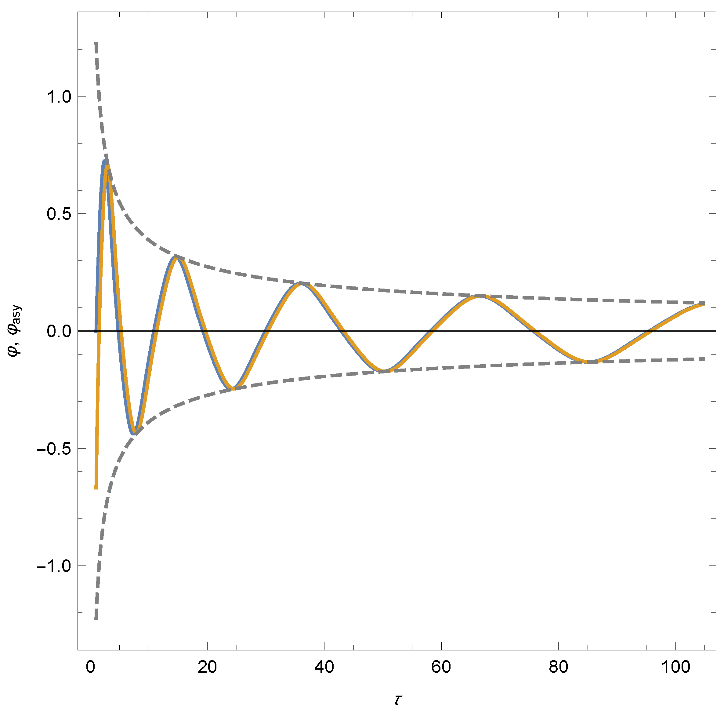
In Figure 3, we plot the results of a numerical integration of the differential Equation (44) with initial conditions $\phi \left(1\right)=0$, ${\phi }^{\prime }\left(1\right)=1$, as well as the leading term of the asymptotic expansion (45). In this case, the dashed lines are the envelopes $\pm {(3/\left(2\tau \right))}^{1/2}$ that set the scale for the generalised asymptotic expansion (45), and the factor ${(3/2)}^{1/2}$ is the prefactor in Equation (53) for ${\phi }_1\left(\tau \right)$.

As in the quadratic case, in Figure 4, we plot three typical asymptotic trajectories on the phase map of the differential Equation (44). Even for arbitrarily large times, the approximation of the representative point to the origin is not monotonic. (In this case, $h\left(\tau \right)$ does not admit the same geometric interpretation as in the quadratic case.)

Again, using Equations (16) and (17), we find the asymptotic formula for the Hubble parameter,

$$H\left(t\right)\sim \frac{1}{2t}-\frac{3m}{{\left(6mt\right)}^{3/2}}\mathrm{sn}\left(s\left(t\right)\right|-1)\mathrm{cn}\left(s\left(t\right)\right|-1)\mathrm{dn}\left(s\left(t\right)\right|-1)+\cdots ,$$

(56)

where

$$s\left(t\right)=\sqrt{6mt}-\sqrt{6m{t}_0},$$

(57)

and using Equation (42), the corresponding formula for the eos parameter,

$$w_{\mathsf{\Phi }}\left(t\right)\sim 1-2\mathrm{sn}{\left(s\left(t\right)\right|-1)}^4+\cdots .$$

(58)

At this order, $w_{\mathsf{\Phi }}\left(t\right)$ is independent of c. In the following section, we show that the leading term of the usual averages of this eos parameter is $1/3$.

4. The General Case

In this section, we discuss the generalised asymptotic solution of Equation (15) for any value of p. The results of this section include as particular cases the quadratic potential $(p=1)$ and the quartic potential $(p=2)$ studied in the previous sections, but the results obtained there were sharper than the results we obtain in this section. In the quadratic case, we could find explicit formulas and a complete asymptotic expansion. In the quartic case, we could still find explicit formulas although we had to limit ourselves to a two-term asymptotic solution. In this section, ${\phi }_1\left(\sigma \right)$ is defined as the solution of an implicit equation.

The general equation, which we repeat here for convenience, is

$${\phi }^{″}\left(\tau \right)+{({\phi }^{\prime }{\left(\tau \right)}^2+\phi {\left(\tau \right)}^{2p})}^{1/2}{\phi }^{\prime }\left(\tau \right)+p\phi {\left(\tau \right)}^{2p-1}=0.$$

(59)

In analogy with the quartic case, we look for a two-term generalised asymptotic solution of the form

$$\phi \left(\tau \right)\sim \frac{{\phi }_1\left(\sigma \right)}{\sigma }+\frac{{\phi }_2\left(\sigma \right)}{{\sigma }^2}+o(1/{\sigma }^2),$$

(60)

where

$$\sigma ={\tau }^{1/p},$$

(61)

and the conditions on the coefficients are the same as in the previous section. By substituting the ansatz (60) into Equation (59), we find the following equations for ${\phi }_1$ and ${\phi }_2$:

$${\phi }_1^{″}+p^3{\left({\phi }_1\right)}^{2p-1}=0,$$

(62)

$${\phi }_2^{″}+p^3(2p-1){\left({\phi }_1\right)}^{2p-2}{\phi }_2=(p+1-{({\left({\phi }_1^{\prime }\right)}^2+p^2{\phi }_1^{2p})}^{1/2}){\phi }_1^{\prime }.$$

(63)

(Again, primes denote derivatives of the functions with respect to their arguments, in this case $\sigma$.)

In general, Equation (62) cannot be solved in closed form. However, it is readily interpreted as the Newton’s equation of motion with respect to the time $\sigma$ of a unit-mass particle with position ${\phi }_1$ under the confining potential $U\left({\phi }_1\right)=p^2{\left({\phi }_1\right)}^{2p}/2$. The corresponding conserved energy is

$$E=\frac{1}{2}{\left({\phi }_1^{\prime }\right)}^2+\frac{p^2}{2}{\left({\phi }_1\right)}^{2p},$$

(64)

and the solution ${\phi }_1\left(\sigma \right)$ is implicitly defined by

$$\sigma -{\sigma }_0={\int }_0^{{\phi }_1}\frac{\mathrm{d}x}{\sqrt{2E-p^2{x}^{2p}}},$$

(65)

or, equivalently, by

$$\sigma -{\sigma }_0=\frac{{\phi }_1}{\sqrt{2E}}{}_2{\mathrm{F}}_1\left(\frac{1}{2},\frac{1}{2p},1+\frac{1}{2p},\frac{p^2}{2E}{\left({\phi }_1\right)}^{2p}\right),$$

(66)

where ${}_2{\mathrm{F}}_1$ denotes the Gauss’ hypergeometric function. Therefore, ${\phi }_1\left(\sigma \right)$ represents a periodic motion on the interval $-{(2E/p^2)}^{1/2p}\le {\phi }_1\le {(2E/p^2)}^{1/2p}$.

Equation (63) is, again, a nonhomogeneous linear differential equation with a non-constant coefficient. Two linearly independent solutions of the homogenous equation are $u_1\left(\sigma \right)={\phi }_1^{\prime }\left(\sigma \right)$ and $u_2\left(\sigma \right)={\phi }_1\left(\sigma \right)+(p-1)\sigma {\phi }_1^{\prime }\left(\sigma \right)$, and, using the method of variation of constants, we find the general solution for ${\phi }_2\left(\sigma \right)$ in terms of ${\phi }_1\left(\sigma \right)$, namely

$$\begin{array}{l}\begin{array}{ll}{\phi }_2\left(\sigma \right)=\hfill & c{\phi }_1^{\prime }\left(\sigma \right)+d({\phi }_1\left(\sigma \right)+(p-1)\sigma {\phi }_1^{\prime }\left(\sigma \right))\hfill \\ & +\left(1-\frac{\sqrt{2E}}{p+1}\right)\left(\sigma {\phi }_1\left(\sigma \right)+\frac{p-1}{2}{\sigma }^2{\phi }_1^{\prime }\left(\sigma \right)\right).\hfill \end{array}\hfill \end{array}$$

(67)

The condition that ${\phi }_2\left(\sigma \right)$ be bounded is that the terms proportional to $\sigma$ and ${\sigma }^2$ vanish, which leads to

$$d=0,E=\frac{1}{2}{(p+1)}^2,$$

(68)

and to

$${\phi }_2\left(\sigma \right)=c{\phi }_1^{\prime }\left(\sigma \right).$$

(69)

We may also determine the first terms of the expansion of the reduced Hubble parameter (17),

$$h\left(\tau \right)\sim \frac{h_1\left(\sigma \right)}{{\sigma }^p}+\frac{h_2\left(\sigma \right)}{{\sigma }^{p+1}}+o(1/{\sigma }^{p+1}),$$

(70)

where

$$h_1\left(\sigma \right)=\frac{1}{p}{({\phi }_1^{\prime }{\left(\sigma \right)}^2+p^2{\phi }_1{\left(\sigma \right)}^{2p})}^{1/2},$$

(71)

$$h_2\left(\sigma \right)=\frac{1}{p^2{h}_1\left(\sigma \right)}({\phi }_1^{\prime }\left(\sigma \right){\phi }_2^{\prime }\left(\sigma \right)+p^3{\phi }_1{\left(\sigma \right)}^{2p-1}{\phi }_2\left(\sigma \right)-{\phi }_1\left(\sigma \right){\phi }_1^{\prime }\left(\sigma \right)).$$

(72)

As a consequence of (62), (64), (68) and (69) we have

$$\begin{array}{lll}{h}_1\left(\sigma \right)\hfill & =& \frac{p+1}{p},\hfill \end{array}$$

(73)

$$\begin{array}{lll}{h}_2\left(\sigma \right)\hfill & =& -\frac{1}{p(p+1)}{\phi }_1\left(\sigma \right){\phi }_1^{\prime }\left(\sigma \right).\hfill \end{array}$$

(74)

Then the leading term of the eos parameter is

$$\begin{array}{lll}{w}_{\mathsf{\Phi }}\left(t\right)\hfill & \sim & \frac{p-1}{p+1}-\frac{2p}{{(p+1)}^2}{h}_2^{\prime }\left(\sigma \right)\hfill \end{array}$$

(75)

$$\begin{array}{lll}\hfill & =& 1-\frac{2p^2}{{(p+1)}^2}{\phi }_1{\left(\sigma \right)}^{2p}.\hfill \end{array}$$

(76)

In particular, the first terms of Equation (43) and of Equation (58) are, respectively, the cases $p=1$ and $p=2$ of Equation (76). That, at this order, $w_{\mathsf{\Phi }}\left(t\right)$ is independent of c is, thus, a general result.

As we mentioned in the introduction, different averaging procedures lead to the same leading contribution of the eos parameter (19). Equation (75) leads to the same result if we average over a period of the variable $\sigma$ as an immediate consequence of this equation and of the periodicity of $h_2\left(\sigma \right)$ in $\sigma$ (see Equation (74)):

$${\langle w_{\mathsf{\Phi }}\rangle }_1=\frac{1}{T_{\sigma }}{\int }_0^{T_{\sigma }}{w}_{\mathsf{\Phi }}\left(\sigma \right)d\sigma \sim \frac{p-1}{p+1}.$$

(77)

It is also easy to derive the same result for other averages used in the literature. For example, Rendall [13] uses the averaging procedure defined by

$${\langle w_{\mathsf{\Phi }}\rangle }_2=\frac{{\displaystyle {\int }_t^{\infty }{p}_{\mathsf{\Phi }}\left(t\right)\mathrm{d}t}}{{\displaystyle {\int }_t^{\infty }{\rho }_{\mathsf{\Phi }}\left(t\right)\mathrm{d}t}}.$$

(78)

In the variable $\tau$,

$$\begin{array}{lll}{p}_{\mathsf{\Phi }}\left(\tau \right)\hfill & =& \frac{M^4}{p}{\left(\frac{2}{3}\right)}^p({\phi }^{\prime }{\left(\tau \right)}^2-\phi {\left(\tau \right)}^{2p}),\hfill \end{array}$$

(79)

$$\begin{array}{lll}{\rho }_{\mathsf{\Phi }}\left(\tau \right)\hfill & =& \frac{M^4}{p}{\left(\frac{2}{3}\right)}^p({\phi }^{\prime }{\left(\tau \right)}^2+\phi {\left(\tau \right)}^{2p}).\hfill \end{array}$$

(80)

Using Equation (18), we find that,

$${\int }_{\tau }^{\infty }{\phi }^{\prime }{\left(\tau \right)}^{2}d\tau =h\left(\tau \right)\sim \frac{p+1}{p}\frac{1}{\tau },$$

(81)

where the asymptotic estimate follows from Equations (70) and (73). Furthermore, using the following consequence of Equations (15) and (17),

$$p\phi {\left(\tau \right)}^{2p}=-h^{\prime }\left(\tau \right)-\frac{1}{2}\phi {\left(\tau \right)}^2{\phi }^{\prime }{\left(\tau \right)}^2-\frac{\mathrm{d}}{\mathrm{d}\tau }\left(\phi \left(\tau \right){\phi }^{\prime }\left(\tau \right)+\frac{1}{2}h\left(\tau \right)\phi {\left(\tau \right)}^2\right),$$

(82)

we note that, as $\tau \to \infty$

$$h\left(\tau \right)\left(1+\frac{1}{2}\phi {\left(\tau \right)}^2\right)=O(1/\tau ),$$

(83)

$$\phi \left(\tau \right){\phi }^{\prime }\left(\tau \right)=O(1/{\tau }^{1+1/p}),$$

(84)

and

$${\int }_{\tau }^{\infty }\phi {\left(\tau \right)}^2{\phi }^{\prime }{\left(\tau \right)}^{2}d\tau =O(1/{\tau }^{1+2/p}).$$

(85)

Therefore,

$${\int }_{\tau }^{\infty }\phi {\left(\tau \right)}^{2p}d\tau \sim \frac{p+1}{p^2}\frac{1}{\tau },$$

(86)

and from (81) and (86), we obtain that

$${\langle w_{\mathsf{\Phi }}\rangle }_2\sim \frac{p-1}{p+1}.$$

(87)

5. Connection between the Oscillatory Period and the Thermalization Period

As we said in the introduction, the oscillatory phase of reheating is an intermediate period between the end of inflation and the beginning of thermalization. Let us denote by $t_{\mathrm{end}}$ the cosmic time corresponding to the end of inflation and by $t_{\mathrm{osc}}$ the cosmic time corresponding to the end of the oscillatory period. There are several criteria to determine the value of the inflaton $\mathsf{\Phi }$ at the end of inflation, which typically give results differing in factors of order unity. For concreteness we quote Equations (2.23) and (2.25) of Ellis et al. [18] for the monomial potentials (11), which, with our conventions, lead to

$$\mathsf{\Phi }\left(t_{\mathrm{end}}\right)=\left(\frac{4p-1}{2\sqrt{2}}\right){\mathrm{M}}_{\mathrm{Pl}},$$

(88)

$$\dot{\mathsf{\Phi }}\left(t_{\mathrm{end}}\right)={\left(\frac{4p-1}{2\sqrt{2}}\right)}^p\frac{M^2}{\sqrt{p}}.$$

(89)

However, these (or similar) values cannot be used directly to relate the parameters ${\sigma }_0$ (or $t_0$) and c in the generalised asymptotic solutions (45) and (60) to the parameters of the model M and p for at least two reasons: First, the translational invariance of the inflaton models and the existence of an attractor in the phase plane [5,19] make it physically dubious relating $t_0$ to a specific moment of physical significance; second, as discussed in Refs [16,20], in general successive terms in generalised asymptotic expansions are not successively smaller at every time: they essentially fix the overall scale of the oscillatory process. (This is the case of $\mathsf{\Phi }\left(t\right)$ and $\dot{\mathsf{\Phi }}\left(t\right)$.)

However, suitable truncations of the generalised expansions may be free or the ambiguities discussed in the previous paragraph and can be used to link the parameter c to the values of physical magnitudes at $t_0$. For concreteness, consider the first two terms of the expansion (40) for $H\left(t\right)$ in the harmonic case, which we repeat here for convenience:

$$H\left(t\right)\sim \frac{2}{3t}+\frac{c+sin\left(2m(t-t_0)\right)}{3m{t}^2}\cdots .$$

(90)

The idea is that the leading term in Equation (90) is not oscillating and, therefore, dominates the following terms at any large time, and that c in the next term is also not multiplied by an oscillating function. Therefore, setting $t=t_0$, we find that

$$c=3m{t}_0^{2}H\left(t_0\right)-2m{t}_0.$$

(91)

Finally, let us briefly discuss the connection between the generalised asymptotic solutions in the oscillatory period to suitable asymptotic solutions in the thermalization period. To this end, we will denote by $t_{\mathrm{osc}}$ the end of the oscillatory period, and by ${\mathsf{\Phi }}_{\mathrm{I}}$ and ${\mathsf{\Phi }}_{\mathrm{II}}$ the respective asymptotic forms of the inflaton field.

We consider first the harmonic case. From (12) and (30), we have that the leading term of the asymptotic expansion (22) is given by

$${\mathsf{\Phi }}_{\mathrm{I}}\left(t\right)=2\sqrt{\frac{2}{3}}{\mathrm{M}}_{\mathrm{Pl}}\frac{cos\left(m(t-t_0)\right)}{mt}.$$

(92)

Furthermore, Equation (10) for the inflaton in the thermalization regime reduces in the harmonic case to

$$\ddot{\mathsf{\Phi }}+\mathsf{\Gamma }\dot{\mathsf{\Phi }}+m^2\mathsf{\Phi }=0,$$

(93)

whose exact solution can be written as

$$\mathsf{\Phi }\left(t\right)=A{\mathrm{e}}^{-\frac{\mathsf{\Gamma }}{2}t}cos\left(\omega (t-t_1)\right),$$

(94)

where

$$\omega =\sqrt{m^2-\frac{{\mathsf{\Gamma }}^2}{4}},$$

(95)

and where A and $t_1$ are arbitrary constants. In addition, for typical situations $m\gg \mathsf{\Gamma }$ and, therefore, $\omega \approx m$. Thus, we take

$${\mathsf{\Phi }}_{\mathrm{II}}\left(t\right)=A{\mathrm{e}}^{-\frac{\mathsf{\Gamma }}{2}t}cos\left(m(t-t_1)\right).$$

(96)

Again, since the expansion (22) is a generalised asymptotic series, by the same arguments used above it is physically meaningful to match the envelopes and the first derivatives of the envelopes of ${\mathsf{\Phi }}_{\mathrm{I}}$ and ${\mathsf{\Phi }}_{\mathrm{II}}$ at $t=t_{\mathrm{osc}}$, instead of matching instantaneous values at a certain time. Thus, we have

$$2\sqrt{\frac{2}{3}}\frac{{\mathrm{M}}_{\mathrm{Pl}}}{m{t}_{\mathrm{osc}}}=A{\mathrm{e}}^{-\frac{\mathsf{\Gamma }}{2}{t}_{\mathrm{osc}}},$$

(97)

$$2\sqrt{\frac{2}{3}}\frac{{\mathrm{M}}_{\mathrm{Pl}}}{m{t}_{\mathrm{osc}}^2}=A\frac{\mathsf{\Gamma }}{2}{\mathrm{e}}^{-\frac{\mathsf{\Gamma }}{2}{t}_{\mathrm{osc}}}.$$

(98)

Hence, we obtain

$$t_{\mathrm{osc}}=\frac{2}{\mathsf{\Gamma }},$$

(99)

and

$$A=\frac{\mathrm{e}}{\sqrt{3}}{\left(\frac{{\mathrm{M}}_{\mathrm{Pl}}}{M}\right)}^2\mathsf{\Gamma }.$$

(100)

Since $\omega \approx m$, we can also set $t_1=t_0$. Moreover, if we approximate the Hubble parameter H by the first term of (40), we obtain the following estimate of $H_{\mathrm{osc}}\equiv H\left(t_{\mathrm{osc}}\right)$,

$$H_{\mathrm{osc}}\approx \frac{\mathsf{\Gamma }}{3}.$$

(101)

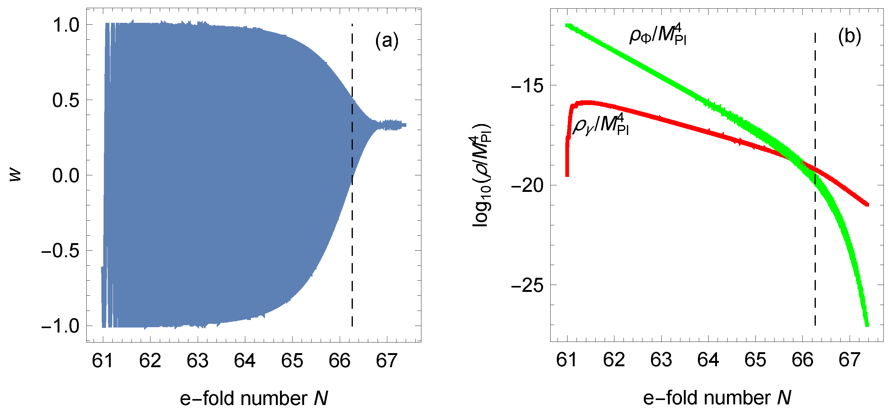
To illustrate graphically the result (99) for $t_{\mathrm{osc}}$, in Figure 5, we present a numerical calculation similar to that of Figure 13 in Ref. [10]. More concretely, we performed a numerical integration of Equations (1)–(6) with the same parameters quoted in the introduction. In Figure 5a, we show the eos parameter (7) as a function of the e-fold number N. The dashed vertical line marks the matching point (99). Perhaps more informative is Figure 5b, in which we show the energy densities of the inflaton (4) and of the radiation as a function of the e-fold number. Again, the dashed vertical line marks the matching point (99), which turns out to be $0.38$ e-folds to the right of the point where the energy densities become equal.

For general p, the first term of the asymptotic expansion (22) is given by

$${\mathsf{\Phi }}_{\mathrm{I}}\left(t\right)=\sqrt{\frac{2}{3}}{\mathrm{M}}_{\mathrm{Pl}}\frac{{\phi }_1\left(\sigma \right)}{\sigma },$$

(102)

where $\sigma ={\left(mt\right)}^{1/p}$ and ${\phi }_1\left(\sigma \right)$ is a periodic function of $\sigma$, which satisfies Equation (62). As a consequence of Equations (64) and (68), ${\phi }_1$ has a maximal amplitude given by ${(1+1/p)}^{1/p}$. Then, from (102), it follows that ${\mathsf{\Phi }}_{\mathrm{I}}$ is a damped oscillatory function of t with envelope given by

$${\mathsf{\Phi }}_{\mathrm{I}}^{\left(\mathrm{env}\right)}\left(t\right)=\sqrt{\frac{2}{3}}{\left(1+\frac{1}{p}\right)}^{1/p}\frac{{\mathrm{M}}_{\mathrm{Pl}}}{{\left(mt\right)}^{1/p}}.$$

(103)

Furthermore, for general p, the Equation (10) for the thermalization regime is a nonlinear Liénard differential equation of the form

$$\ddot{\mathsf{\Phi }}+\mathsf{\Gamma }\dot{\mathsf{\Phi }}+\frac{2M^4}{{\mathrm{M}}_{\mathrm{Pl}}^{2p}}{\mathsf{\Phi }}^{2p-1}=0,$$

(104)

which describes a nonlinear oscillator with linear damping. Cveticanin [19] proved that the approximate solution of this equation describes a vibration with decreasing amplitude of the form (cf. Equations (72) and (73) in Ref. [19])

$${\mathsf{\Phi }}_{\mathrm{II}}^{\left(\mathrm{env}\right)}\left(t\right)=A{\mathrm{e}}^{-\frac{\mathsf{\Gamma }}{p+1}t}.$$

(105)

If we match the envelopes ${\mathsf{\Phi }}_{\mathrm{I}}^{\left(\mathrm{env}\right)}$ and ${\mathsf{\Phi }}_{\mathrm{II}}^{\left(\mathrm{env}\right)}$ and their first derivatives at $t_{\mathrm{osc}}$, we obtain at once

$$t_{\mathrm{osc}}=\left(1+\frac{1}{p}\right)\frac{1}{\mathsf{\Gamma }},$$

(106)

and

$$\begin{array}{lll}A\hfill & =& \sqrt{\frac{2}{3}}{\mathrm{M}}_{\mathrm{Pl}}{\left(\frac{\mathrm{e}\mathsf{\Gamma }}{m}\right)}^{1/p}\hfill \end{array}$$

(107)

$$\begin{array}{lll}& =& {\left(\frac{p}{3}\right)}^{1/\left(2p\right)}\frac{{\mathrm{M}}_{\mathrm{Pl}}^{1+1/p}}{M^{2/p}}{\left(\mathrm{e}\mathsf{\Gamma }\right)}^{1/p}.\hfill \end{array}$$

(108)

In addition, if we approximate the Hubble parameter H by the first term of (70), we obtain the following p-independent estimate of $H_{\mathrm{osc}}$

$$H_{\mathrm{osc}}\approx \frac{\mathsf{\Gamma }}{3}.$$

(109)

Finally, note that the matching of the oscillatory factor for $p>1$, although feasible, is complicated by the fact that the oscillations are not isochronous [19].

6. Conclusions

We analysed the asymptotic properties of the dynamical equation of the inflaton during the oscillatory phase of reheating to extend the existing results for the quadratic case, to provide new explicit results for the quartic case, and implicit results (that include the former as particular cases) for potentials that close to their global minima behave as even monomial potentials.

We paid special attention to the derivation of explicit expressions for the instantaneous eos parameter $w_{\mathsf{\Phi }}$, whose averages turn out to be in agreement with the averaged values found in the literature. Several studies assumed that, during part or the whole reheating period, the constant value $w_{\mathrm{rhe}}\approx \langle w_{\mathsf{\Phi }}\rangle$, thus, neglecting the coupling between the inflaton field and the radiation [10,21,22]. A more realistic yet manageable approach is to use a range of values for $w_{\mathrm{rhe}}$ [23,24]. For instance, a typical range of values for $p=1$ is $0=\langle w_{\mathsf{\Phi }}\rangle \le w_{\mathrm{rhe}}\le 0.25$. In this spirit, our results may be useful to formulate constraints on effective eos parameters $w_{\mathrm{rhe}}$ based on the instantaneous values $w_{\mathsf{\Phi }}\left(t\right)$ rather than on the averaged values $\langle w_{\mathsf{\Phi }}\rangle$.

Finally, as a line of future development, we mention the possible existence of a finer scale than ${\tau }^{1/p}$ that might permit the calculation of full asymptotic expansions for the inflaton, instead of the truncated asymptotic formulas derived in the present paper for the degenerate potentials.