Abstract
The recent data release by the Planck satellite collaboration presents a renewed challenge for modified theories of gravitation. Such theories must be capable of reproducing the observed angular power spectrum of the cosmic microwave background radiation. For modified theories of gravity, an added challenge lies in the fact that standard computational tools do not readily accommodate the features of a theory with a variable gravitational coupling coefficient. An alternative is to use less accurate but more easily modifiable semianalytical approximations to reproduce at least the qualitative features of the angular power spectrum. We extend a calculation that was used previously to demonstrate compatibility between the Scalar–Tensor–Vector–Gravity (STVG) theory, also known by the acronym MOG, and data from the Wilkinson Microwave Anisotropy Probe (WMAP) to show the consistency between the theory and the newly released Planck 2018 data. We find that within the limits of this approximation, the theory accurately reproduces the features of the angular power spectrum.
PACS:
04.20.Cv; 04.50.Kd; 04.80.Cc; 45.20.D-; 45.50.-j; 98.80.-k
1. Introduction
Though highly isotropic, the cosmic microwave background (CMB) shows small temperature fluctuations as a function of the sky direction. The magnitude of these fluctuations depends on the angular size. This location and size of these peaks is an important prediction of the standard model of cosmology, which has been confirmed by increasingly accurate experiments, such as the Boomerang experiment [1], the Wilkinson Microwave Anisotropy Probe (WMAP, [2]), and the Planck satellite [3].
The angular power spectrum of the CMB can be calculated in a variety of ways. The preferred method is to use numerical software, such as CMBFAST [4]. Unfortunately, such software packages cannot be easily adapted for use with a variable-G theory of gravitation, such as the Scalar–Tensor–Vector–Gravity (STVG [5]) theory, also known as MOdified Gravity (MOG).
There are alternative methods of calculation, which, though somewhat less accurate, nonetheless capture the essential qualitative features of the CMB angular power spectrum. The advantage of such calculations is that the physics is transparent and not obscured by “black box” computer code; additionally, the calculations can be adapted with relative ease to accommodate a different theory. One such method is the semianalytical approximation presented in Ref. [6].
We have, in fact, used this approximation in the past showing the agreement between the predictions of the MOG theory and the WMAP results [7,8]. In light of the recently published Planck 2018 results, it is important to revisit and refine this computation and also extend it to high values of the multipole index ℓ.
We begin in Section 2 with a brief introduction to the MOG theory and its acceleration law, which gives rise to the theory’s effective gravitational coupling parameter. In Section 3, we introduce the angular power spectrum and its semianalytical approximation, as presented in Ref. [6] (which the interested reader is advised to consult for details). We adapt the calculation to the MOG theory and show the results. We conclude by presenting our discussion and conclusions in Section 4.
2. The MOG Theory
Our MOG modified gravity theory, also known as Scalar–Tensor–Vector–Gravity (STVG [5]), is a relativistic theory of gravitation based on an action principle. In addition to the metrical field of gravitation, the theory introduces a repulsive vector field of finite range. The gravitational constant and the vector field range (mass) parameter are promoted to dynamical (massless) scalar fields. Within the range of the vector field, the theory replicates Newtonian gravitation; outside this range, in the absence of the repulsive force, gravitation is stronger. By this feature, the theory successfully accounts for galaxy rotation curves [9,10,11,12,13], the matter power spectrum [8], and other cosmological observations [14] while also remaining consistent with recent gravitational wave data [15].
In the weak field, low-velocity regime, the MOG theory yields a simple gravitational acceleration law [16]. For a point source of gravitation characterized by mass M at the origin, the gravitational acceleration at position is given by
with
where is Newton’s constant of gravitation, the dimensionless quantity (i.e., ) characterizes the difference between the theory’s variable gravitational coupling coefficient G and , and is the mass of the vector field.
In an approximately homogeneous and isotropic universe, and can be taken as constants. Consequently, at distance scales characterized by , can be treated as constant as well.
The Friedmann equations that describe a homogeneous and isotropic universe remain valid in the MOG theory [7,8,17,18], with only trivial modifications, which is not surprising given that these equations can also be heuristically derived from the Newtonian theory [6,19]. The equations read (using ):
The critical density, characterized by , , is given by
where .
Note the presence of a factor of in this definition of . Consequently, for a given baryon density , the corresponding density parameter is inflated by this same factor:
Often, in cosmological calculations, is used to represent the baryon density in equations describing both gravitational and nongravitational interactions. Clearly, this convenience is lost in the case of modified gravity in the presence of the factor, which only applies to gravitational interactions.
3. Modeling the Cosmic Microwave Background (CMB)
It is surprisingly difficult to analyze high-quality Cosmic Microwave Background (CMB) data sets from the perspective of a modified gravity theory, such as MOG. The main reason for this difficulty lies in the fact that, as we alluded to above, the dimensionless density parameter is used to represent baryonic matter in calculations that involve gravity as well as calculations that represent nongravitational physics.
Why is this a problem? Consider the definition:
In the standard theory, this expression will suffice. However, what about a theory, such as MOG, with a variable gravitational coefficient ? Clearly, when the context is gravitational, the product accurately reflects the gravitational contribution of baryonic matter. However, when, e.g., the pressure of the medium is considered, is not supposed to be scaled in this manner (pressure does not increase just because gravitation is stronger).
Disentangling these issues in computer codes that have been in use for years or decades, written or rewritten by multiple authors, perhaps even machine-translated from one programming language to another (e.g., from FORTRAN to C) is a daunting task.
Without access to a standard suite of computer programs that can reliably and provably deal with a variable-G modified theory of gravity, we opted for another approach: use a semianalytical approximation that is sufficiently accurate to reproduce the key qualitative features of the CMB angular power spectrum and perhaps even allow us to make some cautious predictions.
Such an approximation method was published by Mukhanov [6]. We previously used this approximation method in the context of WMAP results, showing that MOG indeed fits the angular power spectrum well. In light of the recent release of Planck 2018 data, we found it imperative to revisit and, if necessary, refine this calculation and compare the Planck results against the MOG predictions.
3.1. Semi-Analytical Estimation of CMB Anisotropies
The general expression for the cosmic mean of the CMB temperature autocorrelation function, expressed in terms of multipoles (with the monopole and dipole components, , excluded), can be written as (see Equation (9.38) in [6] and the discussion therein for details):
where is the Fourier-decomposition of the gravitational potential with respect to wavenumber k, is the conformal time at recombination, and corresponds to the present time. The quantity is the fractional energy fluctuation of radiation, defined using the 00-component of the radiation energy-momentum tensor before recombination as , where is the radiation energy density, is the derivative with respect to conformal time, and are the spherical Bessel functions.
For , , ; hence, we find that for , This observation is valid both in the standard -CDM cosmology and the MOG theory, leaving us, for low ℓ, with
If (the extra factor corresponding to a drop of the potential on superhorizon scales after matter-radiation equality), we obtain
Let , , and then,
For large ℓ, still following Ref. [6], we can then write
where we split the eventual solution into oscillatory (O) and non-oscillatory (N) parts.
Using the well-known trigonometric approximations of the spherical Bessel functions for large real arguments, as well as other suitable numerical representations (for details, including the origin of the numerical factors in the equations that follow, consult [6]), we find the following expression for the oscillatory part:
where
and
The non-oscillatory part, in turn, is split into a sum:
where
The parameters that occur in these expressions are as follows. First, the baryon density parameter:
where is the baryon content of the universe at present relative to the critical density, and , with being the Hubble parameter at the present epoch. The growth term of the transfer function is represented by
where is the total matter content (baryonic matter, neutrinos, and cold dark matter). The free-streaming and Silk damping scales are determined, respectively, by
Lastly, the location of the acoustic peaks is determined by the parameter1
Finally, we note that the calculated result for assumes scale invariance. For small deviations from scale invariance characterized as usual by the parameter (with ), the result is scaled:
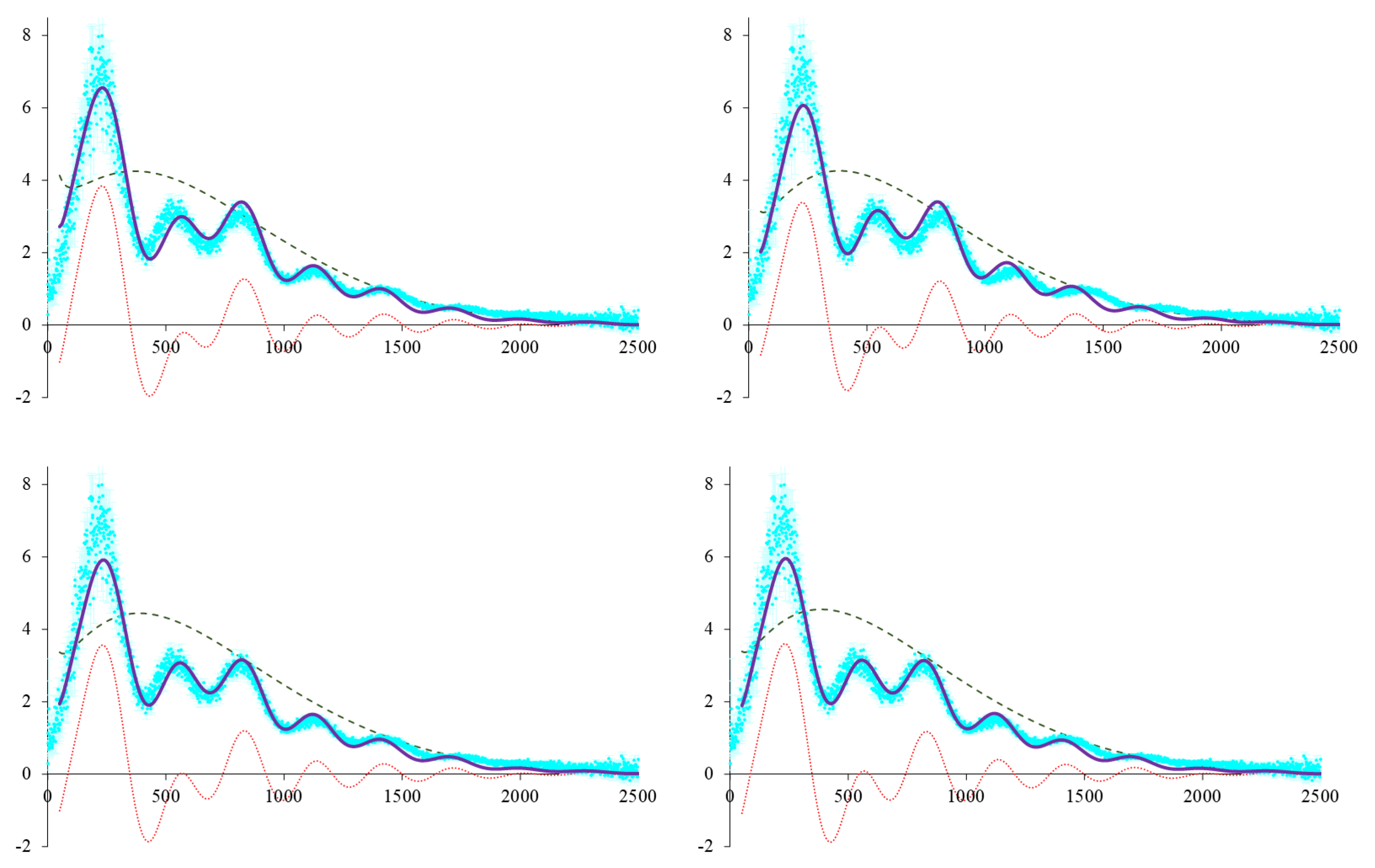
The quality of this approximation is demonstrated in Figure 1 (top left), which shows the estimated angular power spectrum using nominal parameters ( km/s/Mpc, , , with spatially flat cosmology, ) against Planck 2018 data2 from http://pla.esac.esa.int/pla/#cosmology (accessed on 15 September 2021).
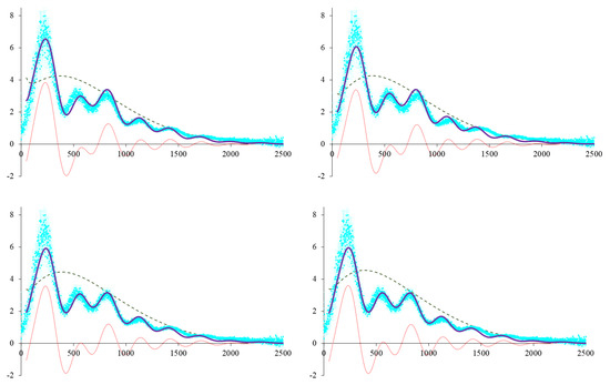
Figure 1.
Mukhanov’s approximation of the angular power spectrum in light of Planck 2018 data. Thick blue line: Mukhanov’s approximation as a sum of an oscillatory part (thin dotted red line) and a nonoscillatory part (dashed green line). Planck 2018 data are shown in light blue with vertical error bars. Top row: standard cosmology, with nominal parameters (left) and least squares fitted values for and (right). Bottom row: The MOG theory, with , and fitted (left) and with the same 3-parameter fit but setting km/s/Mpc fitted (right).
The quality of this fit improves significantly if we allow some of the parameters to vary. For instance, using a simple least squares fit, we obtain , (see Figure 1 top right).
3.2. The MOG CMB Spectrum
What are the key differences between the MOG theory and standard cosmology?
In the standard CDM model in the early universe, there are two main sources of gravitation: baryonic matter and collisionless cold dark matter (CDM). The distribution of matter in the universe is still largely homogeneous, and the gravitational field is determined by the sum .
In the MOG theory, is, of course, absent. However, the gravitational coupling parameter is no longer Newton’s constant. In the late time universe, we expect the gravitational coupling parameter to vary from region to region (an essential feature of the MOG theory that accounts for its ability to model phenomena, such as galaxy rotation curves successfully.) In the early, mostly homogeneous universe, we expect little variation in the value of G; however, .
This means that gravitational interactions are “enhanced” by the factor , defined by the relationship . When computing the results, such as the angular power spectrum, this must be taken into account.
This actually leads to a fairly simple prescription. In the formulation presented in the previous subsection, the density parameter for matter, , must be replaced by .
These changes are, of course, trivial. only appears in Equation (20). For otherwise identical parameterization, we expect identical results.
Instead, we opted to relax the parameter space further as we investigate the MOG solution. Figure 1, bottom left, was obtained by fitting the values of , , and .
As we explored the parameter space, it became evident that there is significant degeneracy with respect to the value of . Figure 1 (lower right) shows another fit, after setting km/s/Mpc, resulting in , , and . We believe that this degeneracy demonstrates the limit of the Mukhanov approximation.
4. Conclusions
Recently, the Planck collaboration released a data set characterizing the cosmic microwave background’s angular power spectrum in more detail than anything previously published. This data release raises the bar for modified theories of gravitation that compete with the standard CDM model as potentially viable representations of the evolution and structure formation in the universe.
We investigated, in particular, the behavior of Scalar–Tensor–Vector–Gravity, also known by the acronym MOG, in light of these new data. A key feature of the MOG theory is the presence of a variable gravitational coupling coefficient, which makes the task of adapting existing numerical models of the CMB or structure formation difficult. Large numerical code bases that are opaque and often use the dimensionless density parameters , , etc., to model both gravitational and nongravitational interactions cannot be easily modified.
Instead, in this paper, we revived a model that we first employed in the wake of the WMAP data release. Extending the calculations to higher multipoles (up to ), we were able to demonstrate that the MOG theory correctly reproduces the qualitative features of the CMB and that within the limits of the approximation, it also produces good quantitative fits. At the same time, we also saw the limitations of the method, notably a degeneracy with respect to . This leads us to conclude that, for instance, to decide whether or not the MOG theory can offer a better resolution to the Hubble tension (see [20] for an up-to-date review), more sophisticated methods will be required.
Acknowledgments
This research was supported in part by Perimeter Institute for Theoretical Physics. Research at Perimeter Institute is supported by the Government of Canada through the Department of Innovation, Science and Economic Development Canada and by the Province of Ontario through the Ministry of Research, Innovation and Science. V.T.T. acknowledges the generous support of Plamen Vasilev and other Patreon patrons.
Conflicts of Interest
The authors declare no conflict of interest.
Notes
| 1 | |
| 2 | For important explanations see https://wiki.cosmos.esa.int/planck-legacy-archive/index.php/CMB_spectrum_%26_Likelihood_Code (accessed on 15 September 2021). |
References
- Jones, W.C.; Ade, P.A.R.; Bock, J.J.; Bond, J.R.; Borrill, J.; Boscaleri, A.; Cabella, P.; Contaldi, C.R.; Crill, B.P.; de Bernardis, P.; et al. A Measurement of the Angular Power Spectrum of the CMB Temperature Anisotropy from the 2003 Flight of BOOMERANG. Astrophys. J. 2006, 647, 823–832. [Google Scholar] [CrossRef] [Green Version]
- Komatsu, E.; Dunkley, J.; Nolta, M.R.; Bennett, C.L.; Gold, B.; Hinshaw, G.; Jarosik, N.; Larson, D.; Limon, M.; Page, L.; et al. Five-Year Wilkinson Microwave Anisotropy Probe Observations: Cosmological Interpretation. Astrophys. J. Suppl. Ser. 2009, 180, 330–376. [Google Scholar] [CrossRef] [Green Version]
- Planck, C.; Aghanim, N.; Akrami, Y.; Ashdown, M.; Aumont, J.; Baccigalupi, C.; Ballardini, M.; Banday, A.J.; Barreiro, R.B.; Bartolo, N.; et al. Planck 2018 results. VI. Cosmological parameters. Astron. Astrophys. 2020, 641, A6. [Google Scholar] [CrossRef] [Green Version]
- Seljak, U.; Zaldarriaga, M. A Line-of-Sight Integration Approach to Cosmic Microwave Background Anisotropies. Astrophys. J. 1996, 469, 437. [Google Scholar] [CrossRef] [Green Version]
- Moffat, J.W. Scalar-tensor-vector gravity theory. J. Cosmol. Astropart. Phys. 2006, 2006, 004. [Google Scholar] [CrossRef]
- Mukhanov, V. Physical Foundations of Cosmology; Cambridge University Press: Cambridge, UK, 2005. [Google Scholar]
- Moffat, J.W.; Toth, V.T. Modified Gravity: Cosmology without dark matter or a cosmological constant. arXiv 2007, arXiv:0710.0364. [Google Scholar]
- Moffat, J.W.; Toth, V.T. Cosmological Observations in a Modified Theory of Gravity (MOG). Galaxies 2013, 1, 65–82. [Google Scholar] [CrossRef] [Green Version]
- Moffat, J.W.; Rahvar, S. The MOG weak field approximation and observational test of galaxy rotation curves. Mon. Not. R. Astron. Soc. 2013, 436, 1439–1451. [Google Scholar] [CrossRef] [Green Version]
- Moffat, J.W.; Toth, V.T. Rotational Velocity Curves in the Milky Way as a Test of Modified Gravity. Phys. Rev. D 2015, 91, 043004. [Google Scholar] [CrossRef] [Green Version]
- Green, M.A.; Moffat, J.W. Modified Gravity (MOG) fits to observed radial acceleration of SPARC galaxies. Phys. Dark Universe 2019, 25, 100323. [Google Scholar] [CrossRef] [Green Version]
- Davari, Z.; Rahvar, S. Testing MOdified Gravity (MOG) theory and dark matter model in Milky Way using the local observables. Mon. Not. R. Astron. Soc. 2020, 496, 3502–3511. [Google Scholar] [CrossRef]
- Moffat, J.W. Gravitational theory of cosmology, galaxies and galaxy clusters. Eur. Phys. J. C 2020, 80, 906. [Google Scholar] [CrossRef]
- Davari, Z.; Rahvar, S. MOG cosmology without dark matter and the cosmological constant. Mon. Not. R. Astron. Soc. 2021, 507, 3387–3399. [Google Scholar] [CrossRef]
- Green, M.A.; Moffat, J.W.; Toth, V.T. Modified Gravity (MOG), the speed of gravitational radiation and the event GW170817/GRB170817A. Phys. Lett. B 2018, 780, 300–302. [Google Scholar] [CrossRef]
- Moffat, J.W.; Toth, V.T. Fundamental parameter-free solutions in Modified Gravity. Class. Quant. Grav. 2009, 26, 085002. [Google Scholar] [CrossRef] [Green Version]
- Toth, V.T. Cosmological consequences of Modified Gravity (MOG). In Proceedings of the International Conference on Two Cosmological Models, Ciudad de Mexico, Mexico, 17–19 November 2010; Auping-Birch, J., Sandoval-Villalbazo, A., Eds.; Universidad Iberoamericana: Ciudad de Mexico, Mexico, 2012; pp. 385–398. [Google Scholar]
- Moffat, J.W. Structure Growth and the CMB in Modified Gravity (MOG). arXiv 2014, arXiv:1409.0853. [Google Scholar]
- Weinberg, S. Cosmology; Oxford University Press: Oxford, UK, 2008. [Google Scholar]
- Di Valentino, E.; Mena, O.; Pan, S.; Visinelli, L.; Yang, W.; Melchiorri, A.; Mota, D.F.; Riess, A.G.; Silk, J. In the Realm of the Hubble tension—A Review of Solutions. arXiv 2021, arXiv:2103.01183. [Google Scholar]
Publisher’s Note: MDPI stays neutral with regard to jurisdictional claims in published maps and institutional affiliations. |
© 2021 by the authors. Licensee MDPI, Basel, Switzerland. This article is an open access article distributed under the terms and conditions of the Creative Commons Attribution (CC BY) license (https://creativecommons.org/licenses/by/4.0/).