Abstract
In this paper we give a brief account of the relations between non-projected supermanifolds and projectivity in supergeometry. Following the general results (L. Sergio et al., 2018), we study an explicit example of non-projected and non-projective supermanifold over the projective plane and show how to embed it into a super Grassmannian. The geometry of super Grassmannians is also reviewed in detail.
1. Introduction: Projectivity and Non-Projectivity in Supergeometry
The problem of projectivity in supergeometry is a long-standing one. Indeed, large classes of complex supermanifolds whose reduced complex manifolds are projective—i.e., there exists an embedding —are known to be non-superprojective (henceforth, projective), that is they do not admit an embedding for some projective superspace This is the case, for example, of a large class of complex super Grassmannians (see [1] and Section 4 of this paper).
The problem of projectivity is related to another central problem characterizing the theory of complex supermanifold, that of the so-called non-projected supermanifolds: these are complex supermanifolds that do not possess a projection to their reduced manifold . Indeed, it has been shown that any projected supermanifold whose reduced manifold is projective, is also superprojective. In other words, if is a projective complex manifolds and is projected, the embedding can be lifted to an embedding of supermanifolds (see for example [2]). Notice that, for this to be true, the existence of the projection map is crucial: indeed, if we let be a very ample line bundle on , then will be very ample on , in the sense that will allow for the embedding at the level of the supermanifolds [2,3].
The story is different when a supermanifold is non-projected. The obstruction theory to find an embedding into projective superspace for a complex supermanifold has been studied for example in [2], back in the early days of supergeometry. There, it is shown that the obstruction to extend the embedding map at the level of the reduced complex manifolds, to an embedding at the level of complex supermanifolds lies in the cohomology groups for and where the vector bundle is constructed via a suitable quotient of the nilpotent bundle of the supermanifold, encoding the behavior of the anti-commutative nilpotent part of the geometry, see [1,3]. This result has some obvious, yet remarkable, consequences: for example, by dimensional reasons, one sees that any supercurve, i.e., any supermanifold of dimension constructed over a projective curve, is actually projective, and the issues regarding projectivity start to arise in dimension , for
Following these considerations, whilst the literature fully acknowledged that in the realm of supergeometry projective superspaces are not as important as they are in ordinary complex algebraic geometry, nothing has been said, by the way, about which sort of space is to be considered when one looks for a universal embedding space for complex supermanifolds. In the recent [4], this problem was taken on starting from dimension , working over the projective plane , and it has been shown that a large class of non-projected complex supermanifolds does not indeed admit projective embeddings, while all of these non-projected and non-projective supermanifolds admit embeddings in some complex super Grassmannians, thus hinting that the same might happen also in higher dimensions.
In the paper, we consider again the problem of embedding a supermanifold into a super Grassmannians, enriching and clarifying the abstract results of [4] by very explicit constructions and examples. In particular, in the first section of the paper, the key concepts of supergeometry are revised and the notation is fixed, and the main result of [4] is reported and put in context as to make the paper self-consistent. Next, following [1], the supergeometry of complex super Grassmannians is explained. In the last section, it is shown how to build maps to super Grassmannians and the example of the dimensional supermanifold over characterized by a decomposable fermionic bundle is carried out in full detail.
The interested reader might find further general references about supergeometry in [1,5,6]. On the problem of projectivity in supergeometry, the reader might refer to [2,7], and the recent [8,9,10].
2. Basics of Supermanifolds
In this section, we recall the basic definitions in the theory of (complex) supermanifolds. The interested reader might find more details in [1] or [3], which we will follow closely. The most important notion in supergeometry is the one of superspace, which is defined as follows.
Definition 1
(Superspace). A superspace is a pair , where is a topological space and is a sheaf of -graded supercommutative rings (super rings for short) defined over and such that the stalks at every point of are local rings.
In other words, a superspace is a locally ringed space having a structure sheaf given by a sheaf of super rings.
The requirement about the stalks being local rings is the same thing as asking that the even component of the stalk is a usual commutative local ring, for in superalgebra one has that if a super ring, then A is local if and only if its even part is (see for example [6]).
It is important to observe that one can always construct a superspace out of two classical data: a topological space, call it again , and a vector bundle over , call it (analogously: a locally free sheaf of -modules). Now, we denote the sheaf of continuous functions (with respect to the given topology) on and we put . The sheaf of sections of the bundle of exterior algebras has an obvious -grading (by taking its natural -grading mod 2); therefore, in order to realize a superspace, it is enough to take the structure sheaf of the superspace to be the sheaf of sections valued in of the bundle of exterior algebras. This is what is called a local model.
Definition 2
(Local Model ). Given a pair , where is a topological space and is a vector bundle over , we call the superspace modeled on the pair , where the structure sheaf is given by the -valued sections of the exterior algebra .
This is a minimal definition of a local model: we have let be no more than a topological space and as such we are only allowed to take to be the sheaf of continuous functions on it. One can obviously work in a richer and more structured category, such as the differentiable, complex analytic, or algebraic category: from now on, we will work in the complex analytic category and we consider local models based on the pair , where is a complex manifold (its underlying topological space will be denoted with and the sheaf of holomorphic functions on with ) and where is a holomorphic vector bundle on . We will call a holomorphic local model a local model constructed on this kind of data.
The concept of a local model enters in the definition of the main character of this paper.
Definition 3
(Complex Supermanifold). A complex supermanifold of dimension is a superspace that is locally isomorphic to some holomorphic local model , where is a complex manifold of dimension n and is a holomorphic vector bundle of rank m.
In other words, if the topological space underlying has a basis , the structure sheaf of the supermanifold is described via a collection of local isomorphisms of sheaves
where we have denoted with the sheaf of sections of the exterior algebra of considered with its -gradation.
In general, given two superspaces, we can define a morphism relating these two.
Definition 4
(Morphisms of Superspaces). Given two superspaces and a morphism is a pair where
- is a continuous map of topological spaces;
- is a morphism of sheaves of-graded rings, having the property that it preserves the-grading and that, given any point, the homomorphismis local, that is it preserves the (unique) maximal ideal,
This definition applies in particular to the case of complex supermanifolds and enters the definition of sub-supermanifolds. Indeed, as in the ordinary theory, a sub-supermanifold is defined in general as a pair , where is a supermanifold and is an injective morphism with some regularity property. In particular, depending on these regularity properties, we can distinguish between two kinds of sub-supermanifolds. We start from the milder notion.
Definition 5
(Immersed Supermanifold). Let be a morphism of supermanifolds. We say that is an immersed supermanifold if is injective and the differential is injective for all
Making stronger requests, we can give instead the following definition.
Definition 6
(Embedded Supermanifold). Let be a morphism of supermanifolds. We say that is an embedded supermanifold if it is an immersed submanifold and is an homeomorphism onto its image.
In particular, ifis a closed subset ofwe will say thatis a closed embedded supermanifold.
In what follows, we will always deal with closed embedded supermanifolds. Remarkably, it is possible to show that a morphism is an embedding if and only if the corresponding morphism is a surjective morphism of sheaves. Notice that, for example, given a supermanifold one always has a natural closed embedding: the map , which embeds the reduced manifold underlying the supermanifold into the supermanifold itself.
We now introduce some further pieces of information carried by a supermanifold.
Definition 7
(Nilpotent Sheaf/Fermionic Sheaf). We call the nilpotent sheaf the sheaf of ideals of generated by all of the nilpotent sections, that is we put .
We also call fermionic sheafthe locally free sheaf of-module of rankgiven by the quotient.
It is crucial to note that modding out all of the nilpotent sections from the structure sheaf of the supermanifold , we recover the structure sheaf of the underlying ordinary complex manifold that the local model was based on. We call the complex manifold the reduced manifold of the supermanifold loosely speaking, the reduced manifold arises by setting all of the nilpotents in to zero.
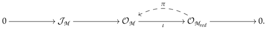
In other words, more invariantly, attached to any complex supermanifold, there is a short exact sequence that relates the supermanifold with its reduced manifold:
where and the surjective sheaf morphism corresponds to the existence of an embedding of the reduced manifold inside the supermanifold . Notice that , where is the surjective sheaf morphism in Equation (2).
We will refer to the short exact sequence of Equation (2) as the structural exact sequence of .
A very natural question arising when looking at the structural exact sequence of Equation (2) associated to a certain supermanifold is whether it is a split exact sequence or not, that is whether there exists a retraction—called projection in this context— such that
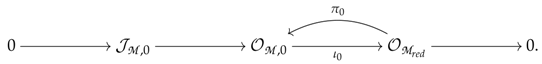
Notice that, more precisely, this shall be recast into the splitting of two exact sequences—the even and the odd part of Equation (2), as we are only dealing with parity preserving morphisms. In particular, we shall give the following definition.
Definition 8
(Projected Supermanifold). We say that a supermanifold is projected if the even part of its structural exact sequence of Equation (2) splits:
It is important to observe that, if the structure sheaf of a supermanifold is a sheaf of -modules if and only if the supermanifold is projected, indeed in this case one has that is this case the theory simplifies considerably as all of the sheaves of -modules defined on the supermanifold are also sheaves of -modules.
Notably, if also the odd part of the structural exact sequence attached to the supermanifold is split, that is
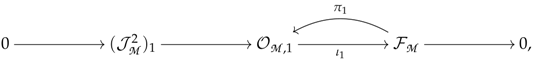 then the supermanifold is called split: this expresses in a more invariant and meaningful form the isomorphism the supermanifold is globally isomorphic to the local model onto which it is based. In other words, we might say that a supermanifold is split if and only if it is projected and the short exact sequence of Equation (5) is split. There indeed exists projected supermanifolds that are not split.
Notice that all of the complex supermanifolds having odd dimension 1 are projected and split for dimensional reasons. When going up to odd dimension 2 a supermanifold can instead be non-projected—the short exact sequence of Equation (4) indicates that is an extension of by the line bundle . If we call a supermanifold a complex supermanifold having an odd dimension equal to 2, we have the following important result.
Theorem 1
( = 2 Supermanifolds). Let be a supermanifold. Then is defined up to an isomorphism by the triple where is a rank sheaf of locally free -modules, the fermionic sheaf of , and The supermanifold is non-projected if and only if .
The proof of the statement can be originally found in [1] and has been reproduced in full detail in [3].
3. Non-Projected Supermanifolds over
Using Theorem 1 of the previous section, in the recent [4], all the non-projected supermanifolds over the projective plane were described through their characterizing cohomological invariants and their transition functions have been given. These non-projected supermanifolds reveal interesting features.
We first set out conventions: we consider a set of homogeneous coordinates on and the set of the affine coordinates and their algebras over the three open sets of the covering of . In particular, modulo , we have the following
The transition functions between these charts reads
We also denote a basis of the rank locally free sheaf on any of the open sets , for , and, since , the transition functions among these bases will have the form
with a matrix with coefficients in . Note that in the transformation of Equation (8) one can write as a matrix with coefficients given by some even rational functions of , because of the definitions (6) and the facts that and .
Finally we note the transformation law for the products is given by
Since is a transition function for the invertible sheaf over , this can be written, up to constant changes of bases in and , in the more precise form
Thus, we can identify the base of with the standard base of over .
Having set these conventions and notations, we can give the following theorem, whose detailed proof can be found in [4].
Theorem 2
(Non-Projected = 2 Supermanifolds over 𝕡2). Every non-projected supermanifold over is characterized up to isomorphism by a triple where is a rank sheaf of -modules such that and ω is a non-zero cohomology class .
The transition functions for an element of the familyfrom coordinates onto coordinates onare given by
whereis a representative of the classand M is amatrix with coefficients insuch that.
Similar transformations hold between the other pairs of open sets.
We remark that the form of transition functions above is shared by all the supermanifolds , regardless the form of its fermionic sheaf , which is encoded in the matrix M.
Some remarkable properties of this family of non-projected supermanifolds has been given by the authors in [4]. We condensate these results in the following theorem.
Theorem 3.
Let be a non-projected supermanifold in the familyThen
- is non-projective, that is cannot be embedded into any projective superspace of the kind;
- can be embedded into a super Grassmannian.In particular, letbe the tangent sheaf of , if we let, for anythe evaluation mapinduces an embedding:
We observe that the theorem proves the existence of an embedding into some super Grassmannian, but it is not effective in that it does not give an esteem of the symmetric power of the tangent sheaf needed in order to set up the embedding. In the next sections, we will first review the geometry of super Grassmannians, and we will then treat explicitly an interesting example of embedding into a super Grassmannian, by choosing a decomposable fermionic sheaf satisfying the hypotheses of Theorem 2.
4. Elements of Super Grassmannians
This section is dedicated to the introduction of some elements of geometry of super Grassmannians. We remark that this section contains no original result and it is fully expository: all of the results are originally due to Y. Manin and his school, see in particular [1,5,7]. Nonetheless, we believe that since the cited literature is somewhat difficult and largely sketchy in the proofs of the various statements, it might be useful to have the constructions revised and readily at hand. In the present section, our emphasis will be on the non-projectedness and non-projectivity issues.
Super Grassmannians are the supergeometric generalization of the ordinary Grassmannians. This means that is a universal parameter space for -dimensional linear subspaces of a given -dimensional space . We will deal with the simplest possible situation, choosing the -dimensional space to be a super vector space of the kind .
We start reviewing how to construct a super Grassmannian by patching together the “charts” that cover it: this is nothing but a generalization of the usual construction of ordinary Grassmannians making use of the so-called big cells.
- We let be such that and look at as given by . This is obviously freely generated, and we will write its elements as row vectors with respect to a certain basis, where the upper indices refer to the -parity.
- Consider a collection of indices such that is a collection of out of the n indices of and is a collection of indices out of m indices of . If is the set of such collections of indices I one obtainsThis will give the number of super big cells covering the super Grassmannian.
- Choosing an element , we associate to it a set of even and odd (complex) variables, we call them . These are arranged as to fill in the places of a matrix a way such that the columns having indices in forms a unit matrix if brought together. To make this clear, for example, a certain choice of yields the followingwhere we have chosen to pick that particular that underlines the presence of the unit matrix.
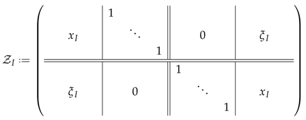
- We now define the superspace to be the analytic superspace , where are the complex coordinates over the point. Whenever represented as above, the superspace related to is called a super big cell of the Grassmannian, and denoted with or, again, simply by (which encodes the topological information).
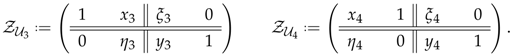
- We now show how to patch together two superspaces and for two different . If is the super big cell related to , we consider the super submatrix formed by the columns having indices in J. Let be the (maximal) sub-superspace of such that on the submatrix is invertible. As usual, the odd coordinates do not affect the invertibility, so it is enough that the two determinants of the even parts of the matrix (that are, respectively, a and a matrix) are different from zero. When this is the case, on the superspace , one has common coordinates and , and the rule to pass from one system of coordinates to the other one is provided byFor example, let us consider the following two super big cells:
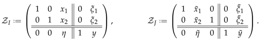 Looking at , we see that the columns belonging to J are the first, the third, and the fourth, so thatWhen computing the determinant of the upper-right matrix, the invertibility of corresponds to (as seen from the point of view of . Likewise one would have found by looking at and ). The inverse of isso that we can compute the coordinates of as functions of the ones of via the rule :so that the change of coordinates can be read out of this. Observe that the denominator is indeed invertible on
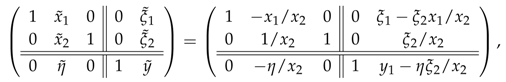
- Patching together the superspaces , one obtains the Grassmannian supermanifold as the quotient supermanifoldwhere we have written for the equivalence relations generated by the change of coordinates that have been described above. Notice that, as a (complex) supermanifold, a super Grassmannian has dimensionWe stress that the maps are isomorphisms onto (open) sub-superspaces of the super Grassmannian, so that the various super big cells offer a local description of it, in the same way a usual (complex) supermanifold is locally isomorphic to a superspace of the kind
Clearly, the easiest possible example of super Grassmannians are projective superspaces that are realized as , exactly as in the ordinary case: these are split supermanifolds, a feature that they do not in general share with a generic Grassmannian , as we shall see in a moment.
For convenience, in what follows we call G a super Grassmannian of the kind and we give the following, see [1].
Definition 9
(Tautological Sheaf on a Super Grassmannian). Let G be a super Grassmannian and let it be covered by the super big cells . We call tautological sheaf of the super Grassmannian G the sheaf of locally free -modules of rank defined as
Notice that this definition is well-posed, since one has that and are identified by means of the transition functions
One can have insights about the geometry of a super Grassmannian by looking at its reduced space—which, we recall, encloses all the topological information—and at the filtration of its trivial sheaf .
We start observing that, given a super Grassmannian G, one automatically has two ordinary even sub-Grassmannians.
Definition 10
(G0 and G1). Let be a super Grassmannian. Then we call and the two purely even sub-Grassmannians defined as
Given a super big cell , and can be visualized as the upper-left and the lower-right parts, respectively, and they come endowed with their tautological sheaves. We call them and . Notice, though, that defines a sheaf of locally free -modules and, as such, it has rank .
Let us now consider an ordinary even complex Grassmannian G of the kind together with its tautological sheaf . One can then also define the sheaf orthogonal to the tautological sheaf, we call it , whose dual fits into the short exact sequence
Notice that in the case the Grassmannian corresponds to a certain projective space , the sheaf orthogonal to the tautological sheaf can be read off the Euler exact sequence twisted by the tautological sheaf itself , and, indeed, we have that , so that
In the case of a super Grassmannian , the sequence (23) is generalized to the canonical sequence
Recalling that and , we now have all the ingredients to state the following theorem, whose proof is contained in [1].
Theorem 4.
Letbe a super Grassmannian, and letandbe their even sub-Grassmannians together with the sheaves, and. Then the following (canonical) isomorphisms hold true:
- (1)
- ;
- (2)
- ,
where bywe mean the super-symmetric algebra over.
The fundamental example, yet enclosing all the features characterizing the peculiar geometry of super Grassmannians, is given by —which is of dimension . We now study its geometry in some detail.
The Geometry of: We start studying the geometry of , G for short, from its reduced manifold, which is easily identified using the previous Theorem 4.
Lemma 1
(). Let G be the super Grassmannian as above. Then
Proof.
Keeping the same notation as above, one obtains and . Therefore, topologically, one has and , where the subscripts refer to the two copies of projective lines. The conclusion follows by the first point of the previous theorem. □
It is fair to observe that we would have arrived at the same conclusion by looking at the big cells of this super Grassmannian, after having set the nilpotents to zero.
We thus have the following situation
 that helps us to recover the geometric data of and G out of those of the two copies of projective lines.
Along this line, we recall that is the external tensor product . Since the tautological sheaf on is we have that
Similarly, observing that the sheaf dual to the tautological sheaf on is given again by the sheaf , as the (twisted) Euler sequence reads
and therefore one has the following:
This is enough to identify the fermionic sheaf of G, since . Therefore, by virtue of the second point of the previous Theorem 4, one has , so
which, in turns, shows that
and one can prove the following.
Theorem 5
( is Non-Projected). The supermanifold is in general non-projected. In particular,
Proof.
In order to compute the cohomology group , we observe that in general, on the product of two varieties, we have , where the are the projections on the factors, so that, in particular, we find
Taking the tensor product with , one has
Now, by the Künneth formula, one has
so that
which concludes the proof. □
There are different ways to find the representatives in the obstruction cohomology group for G. We will first use the super big cells of to identifies these representatives and to establish that in the isomorphisms , the cohomology class corresponds to the choice . This is an explicit and immediate way to do this.
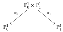
First, we observe that, since the reduced manifold underlying has the topology of , it is covered by four open sets. If we call the usual open sets covering and , the open sets covering , we then have a system of open sets covering their product given by
These correspond to the following matrices , out of which we can read the coordinates on the big cells:
Following the procedure illustrated above or by rows and columns operations on the , one finds the transition rules between the various charts:
By looking at these transformation rules, we therefore have that, in the isomorphism above, the class is represented by and the cocycles representing are given by where the are (in tensor notation)
One can arrive at the same result by means of a different computation, as remarked above. Observing that is generated by the two elements
we can then look at these generators in the intersections, keeping in mind that in order to identify the cocycles that enter in the transition functions. We examine the various intersections.
- : The following identifications can be made:These yield the transition functions above between and and between and . Notice that, in the intersection , only the bit contributes. We have thereforewhere we have denoted by ⊙ the supersymmetric product of the two (local) sections on as represented above.
- : Here we have a contribution from only and, therefore, we have to deal with . By a completely analogous treatment as above, one finds that
- : In this case, we have both contributions, soso that by analogous manipulations as the one above one finds
All the other are identified in the same way and enter one of these three categories.
To conclude, one then imposes the cocycle conditions as to fix the various signs of the and above, which agrees with the one we found above by looking at the coordinates of the big cells: choosing —this can always be done up to a change of coordinates—one obtains the same even transition functions as above.
This is enough to use the theorem classifying the complex supermanifold of dimension (see [1] or [4]) as to conclude that can be defined up to isomorphism as follows.
Definition 11
() as a Non-Projected Supermanifold). The super Grassmnannian can be defined up to isomorphism as the dimensional supermanifold characterized by the triple , where and where , with and , in the isomorphism .
On a very general ground, apart from projective superspaces, super Grassmannians are in general non-projected: the case of we treated is the first non-trivial example of non-projected super Grassmannian.
Now, we jump to the second issue we are interested in: We show that is not a projective supermanifold.
Theorem 6
( is Non-Projective). Let be super Grassmannian defined as above. Then is non-projective.
Proof.
In order to prove the non-projectivity of , we consider the following short exact sequence that comes from the structural exact sequence of G:
Ordinary results in algebraic geometry yield , whereas Likewise, one has and by means of the ordinary exponential exact sequence. This is enough to realize that the cohomology sequence induced by the sequence above splits into two exact sequences. The first one gives an isomorphism , while the second one instead reads
Thus, in order to establish the fate of the cohomology group , one has to look at the boundary map . Let us then consider the following diagram of cochain complexes:
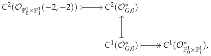 obtained by combining Equation (48) with the Čech cochain complexes of the sheaves that appear.
Since , given the usual cover of by the open sets above, could be represented by (six) cocycles . Explicitly, these cocycles are the transition functions of the line bundle
where, with an abuse of notation, we dismiss the second bit of the external tensor product, which is just the identity. Since the map is surjective, these cocycles are images of elements in . Notice that j is induced by the inclusion of the reduced variety into G, so the cochains in are exactly the we have written above (notice also that these are no longer cocycles in ). Using the Čech coboundary map over G, one finds, for example,
Indeed, by looking at the affine coordinates in the big cells, these read . Setting, as we have done above,
and taking their supersymmetric product, one has . Now, by exactness of the diagram, this element is in the kernel of the map , which equals the image of the map , therefore there exists an element such that and it is a cocycle. Then, considering that the map i is induced by the map , we have that the element is the image of via i. By symmetry, the same applies to the second generator of , which is given by ; thus, the map reads By exactness, it follows that the only invertible sheaves on that lift to the whole G are those of the kind , as the composition of the maps yields as it should. Since these invertible sheaves have no cohomology, they cannot give any embedding in projective superspaces, and this completes the proof. □
Notice the subtlety: the above theorem says that (actually ), but still there are no ample invertible sheaves that allow for an embedding of into some projective superspaces.
The fundamental consequence is that non-projectivity is not confined to this particular super Grassmannian only.
Theorem 7
(Super Grassmannians are Non-Projective). The super Grassmannian space for and is non-projective.
Proof.
As in [1], it is enough to observe that the inclusion induces in turn the inclusion . This last super Grassmannian is isomorphic, as for the usual Grassmannians, to , which in turn embeds into . This leads to as is non-projective, and so is , completing the proof. □
The upshot of this result is that, working in the context of algebraic supergeometry, it is no longer true that projective superspaces are a privileged ambient: this is a substantial departure from usual context of complex algebraic geometry, which deserves to be stressed out.
5. Maps and Embeddings into a Super Grassmannian: An Explicit Example
Having reviewed the geometry of super Grassmannians in the previous section, we now consider the problem of setting up maps to super Grassmannians.
First we recall the universal property characterizing the construction of maps into projective superspaces , which is nothing but a direct generalization of the usual criterium in algebraic geometry for projective spaces , using invertible sheaves, i.e., for any supermanifold or superscheme , any locally free sheaf of rank on and any vector superspace V having a surjective sheaf-theoretical map , then there exists a unique (up to isomorphisms) map such that the inclusion is the pull-back of the inclusion coming from the Euler exact sequence. More concretely, this is sometimes reported simply asking to be globally generated, which means that there exists a surjective sheaf-theoretical map , with . If this is the case, there exists a unique map up to isomorphism such that and such that, if , then and for and , where are the generating sections of , where we recall also that . See [11], where invertible sheaves on projective superspaces are studied.
A very similar situation happens in the case of super Grassmannians, but instead of invertible sheaves one has to deal with locally free sheaves of higher rank/vector bundles, in order to appropriately set up maps. Indeed, let be a super Grassmannian. Then it is has the following universal property that characterizes the maps toward it [4]:
Universal Property:
For any supermanifold or superscheme , any locally free sheaf of -modules of rank on and any vector superspace V with a surjective sheaf-theoretical map , there exists a unique map such that the inclusion is the pull-back of the inclusion from the sequence
where is the tautological sheaf of the super Grassmannian.
Using the universal property above, we now explicitly show that there exists a map from a non-projected non-projective supermanifold of the family , namely that one characterized by the decomposable fermionic sheaf , to a certain super Grassmannian, namely
For future use, we start giving in the following lemma the explicit form of the transition functions of this supermanifold in the case one chooses a decomposable fermionic sheaf, as the one above.
Lemma 2
(Transition functions). Let be the non-projected supermanifold with . Then its transition functions take the following form:
Proof.
The conclusion follows immediately from Theorem 2, taking into account the transition matrix for the given , which have the form on and a similar form on the other two intersections of the fundamental open sets. □
Now we have to identify a suitable locally free sheaf to set up the map into the super Grassmannian: A natural choice is given by the tangent sheaf of —which is obviously a rank locally free sheaf in the case we are dealing with—and, possibly, its higher-symmetric powers we will see that, in this case, is actually enough and one does not need to resort to its higher symmetric products.
In the following, we will show that the vector superspace of global sections of the tangent sheaf , that is the 0-Čech cohomology space , is isomorphic to and that one has a surjective map that is the tangent sheaf is globally generated. As in the universal property above, this implies that the choices of the tangent sheaf for and of for V lead to the existence of a (unique) map
In order to prove the above statement, one needs to carefully study the tangent sheaf . We start considering the restriction of the tangent sheaf to the reduced manifold , that is
It is a general result that , see for example [1] or [3]. This result can be readily read off once one has the explicit form of the transition functions of the tangent sheaf. Indeed, using the chain rule and starting from the above lemma, with obvious notation, one finds
so that the related Jacobian has the following matrix representation
The transition functions in the other intersections can be found by -symmetry.
We now recall that, having at disposal the structure sheaf of , we can also form a sub-superscheme of through the pair . We stress that this is not a supermanifold: indeed it fails to be locally isomorphic to any local model of the kind : more generally, it is locally isomorphic to an affine superscheme for some super ring. We call the superscheme defined by the pair and we characterize its geometry in the following lemma.
Lemma 3
(The Superscheme ). Let be the superscheme as above. Then is a projected scheme and its structure sheaf is given by a locally free sheaf of -algebras such that
Proof.
It is enough to observe that the parity splitting of the structure sheaf reads , so the defining short exact sequence for the even part reduces to an isomorphism . The structure sheaf is endowed with a structure of -module given by , which actually coincides with the parity splitting.
We observe that in the -algebra , the product is null. □
Pushing the characterization of the tangent sheaf a little bit further, we have to study the geometry of tangent bundle when restricted to the sub-superscheme . Once again, it can be proved that the following general isomorphism holds true:
where the first two summands are the even part and the second two summands are the odd part of the sheaf. In particular, in our case one obtains.
Lemma 4
(The Sheaf ). The sheaf is a locally free of -module; moreover, the following isomorphism holds:
Proof.
The claim is proved by computing
where we have used that, since is a locally free sheaf of -module, we have that . The first isomorphism is a standard result in modules theory (note we have suppressed the subscript in the sheaf of nilpotent element for a better notation). □
For computational purposes, the sheaf can be made more explicit in its -module structure, indeed by making explicit its components, one finds
This decomposition will be useful once we have to compute the cohomology.
In order to compute the number of the global sections of the tangent sheaf of , to identify the supposed target super Grassmannian, we actually need one further sheaf, which we will study in the following lemma.
Lemma 5
(The Sheaf ⊗ ). The sheaf is isomorphic to . Moreover, it is a locally free sheaf of -modules and, as such, it is isomorphic to .
Proof.
First of all we recall that is a -module as it is killed by multiplication by . Moreover, the tangent sheaf is locally free and is therefore flat, so the functor is exact. Let us then consider the short exact sequence
By tensoring with , we obtain the short exact sequence
which implies that is indeed isomorphic to . Moreover, we have that , and, as such, it is a -module. Moreover, since , we have that □
We are now in the position to study the global sections of the tangent sheaf . The main tool we will use is the following exact sequence:
together with its long cohomology exact sequence. The previous lemmas together yield the following result.
Lemma 6.
The zeroth and the first cohomology groups of the sheavesandare given by
Proof.
The result follows from a straightforward computation, once given the decomposition into direct sums of the sheaves above. □
We are thus led to the following theorem, which is the main step toward the realization of an embedding into a super Grassmannian.
Theorem 8
(Global Sections of ). The tangent sheaf of has global sections.
Proof.
Using the results of the previous lemma, the long exact cohomology sequence given by (64) reads
Therefore, since is 1-dimensional, in order to prove surjectivity of the connection homomorphism , it is enough to show that it is not zero. To this end, we observe that in the decomposition (62), there is a term of the kind . It is easy to realize that the corresponding global sections are of the form
which we write multiplicatively as and (both taken ). Indeed, changing coordinates, by means of the transformation rules obtained above, we obtain, for example,
and, on the other hand, we have
That is, we have that Now, observing that , we conclude that
represents the same cocycle of that determines the non-vanishing class , as we have described early on. Observing that , we conclude that the connecting homomorphism is non-null and hence surjective. This splits the first part of the cohomology long exact sequence above in two pieces. In particular, we have
which proves that . □
We are left to prove that the tangent sheaf is actually globally generated. This is achieved in the following lemma.
Lemma 7
( is globally generated). The tangent sheaf of is such that the evaluation map is surjective. That is, is globally generated.
Proof.
We let and V be its complement into , so that , and we call . We have the following commutative diagram:
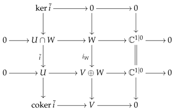 where corresponds to , as computed above. Then, by snake lemma, we have an exact sequence:
Therefore, , and we have a surjection . In particular, since , we have a surjective map . Now, let us consider the evaluation map , which is a homomorphism of locally free sheaves of -modules. Upon using Nakayama Lemma (see for example [6]), it is enough to show that for all , the linear map
which sends a global section s to its evaluation in is surjective. This map can in turn be factored through as follows:
where corresponds to , as computed above. Then, by snake lemma, we have an exact sequence:
Therefore, , and we have a surjection . In particular, since , we have a surjective map . Now, let us consider the evaluation map , which is a homomorphism of locally free sheaves of -modules. Upon using Nakayama Lemma (see for example [6]), it is enough to show that for all , the linear map
which sends a global section s to its evaluation in is surjective. This map can in turn be factored through as follows:
Then, the first one has been just shown to be surjective, while the second one is well-known to be surjective as is a direct sum of globally generated sheaves of -modules. This concludes the proof. □
The universal property, thus leads to the following.
Theorem 9
(Map to ). There exists a unique map up to isomorphism.
More can be said about this map, which is actually an embedding of into : that is, it is an injective map, and its differential is injective as well. We prove this in a completely explicit fashion by realizing the actual embedding in a certain chart.
We explain the strategy to do this in a general setting: once one has a map into a super Grassmannian and a local basis is fixed for over some open set , then, over , the evaluation map is defined by a matrix with coefficients in , and any reduction of into a standard form of type
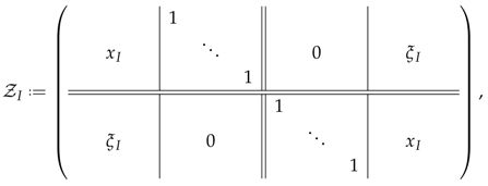 by means of elementary row operations, is a local representation of the map . One can then easily verify injectivity and the injectivity of the differential of this map via this local representation, to establish whether the map constitutes an embedding.
In order to do this, we need the explicit form of the global sections generating . Notice that, to keep the discussion as general as possible we will keep a parameter representing the cohomology class , which we recall to be the same appearing in the transition functions provided by Theorem 2.
Theorem 10
(Generators of ). The tangent sheaf of has global sections and in particular, in the local chart , a basis for is given by , where
where is a complex number representing the cohomology class .
Proof.
The theorem is proved by evaluating the 0-Čech cohomology group of , by means of a computation in charts. □
Now, following that explained above, the coefficients of the expansion are mapped into columns, so that the resulting matrix is a super Grassmannian of the kind , represented in a certain super big-cell. The full super Grassmannian is then reconstructed via its transition functions, as explained in the previous section.
In our particular case, the global sections lead to an image into as follows:
where we have highlighted the super big-cell singled out by the four global sections in the chart , and the for , make up four matrices:
where the subscript referring to the chart of has been suppressed for readability purpose. One can then confirm that the map is indeed an embedding via this explicit expression.
Theorem 11.
Letbe the non-projected supermanifold endowed with a fermionic sheaf. The map thenis an embedding of supermanifolds.
Proof.
One can check from the expressions above that the map is injective on the geometric points, that is on , and that its super differential is injective. This can be checked, for example, by representing the super differential as a matrix, where the four rows are given by the derivatives of a row vector with respect to The resulting matrix has indeed Rank 4. □
It is fair to say that one can simplify the proof and avoid cumbersome computation, by considering just a subset of the global sections found above in order to prove global generation and injectivity of the differential. For example, the subset of given by the sections
does the job. Indeed, these sections make up a sub-matrix of the matrix given, having columns given by coordinates of the global sections with respect to the basis in the chart as above. Writing the columns in a suitable order, one obtains
This is a linear embedding of into a super big-cell of the super Grassmannian, which proves both global generation and injectivity at the level of the differential over at once. Additionally, by symmetry, or analogously by the homogeneity of and with respect to the action of , the same result holds true over and as well.
Funding
This research received no external funding.
Acknowledgments
The author would like to thank the anonymous reviewers for their useful comments. This research is original and has a financial support of the Università del Piemonte Orientale (Fondi Ricerca Locale).
Conflicts of Interest
The author declares no conflict of interest.
References
- Manin, Y.I. Gauge Fields and Complex Geometry; Springer: Berlin/Heidelberg, Germany, 1988. [Google Scholar]
- LeBrun, C.; Poon, Y.-S.; Wells, R.O., Jr. Projective Embedding of Complex Supermanifolds. Comm. Math. Phys. 1990, 126, 433–452. [Google Scholar] [CrossRef]
- Noja, S. Topics in Algebraic Supergeometry over Projective Spaces. Ph.D. Thesis, Università degli Studi di Milano, Milano, Italy, 2018. [Google Scholar]
- Cacciatori, S.L.; Noja, S.; Re, R. Non Projected Calabi-Yau Supermanifolds over 𝕡2. arXiv, 2018; arXiv:1706.01354. [Google Scholar]
- Manin, Y.I. Topics in Noncommutative Geometry; Princeton University Press: Princeton, NJ, USA, 1991. [Google Scholar]
- Varadarajan, V.S. Supersymmetry for Mathematicians: An Introduction; Courant Lecture Notes; American Mathematical Society (AMS): Providence, RI, USA, 2004; Volume 11. [Google Scholar]
- Penkov, I.B.; Skornyakov, I. Projectivity and D-affinity of Flag Supermanifolds. Uspekhi Math. Nauk. 1985, 40, 211–212. [Google Scholar] [CrossRef]
- Bettadapura, K. Embeddings of Complex Supermanifolds. arXiv, 2018; arXiv:1806.02763. [Google Scholar]
- Fioresi, R.; Latini, E.; Lledo, M.A.; Nadal, F.A. The Segre embedding of the quantum conformal superspace. arXiv, 2017; arXiv:1709.03075. [Google Scholar]
- Noja, S. Supergeometry of Π-Projective Spaces. J. Geom. Phys. 2018, 124, 286–299. [Google Scholar] [CrossRef]
- Cacciatori, S.L.; Noja, S. Projective Superspaces in Practice. J. Geom. Phys. 2018, 130, 40–62. [Google Scholar] [CrossRef]
© 2018 by the author. Licensee MDPI, Basel, Switzerland. This article is an open access article distributed under the terms and conditions of the Creative Commons Attribution (CC BY) license (http://creativecommons.org/licenses/by/4.0/).