Primordial Gravitational Wave Birefringence in a de Sitter Background with Chern–Simons Coupling

Abstract

In this work, we investigate tensor perturbations in a de Sitter background within the framework of Chern–Simons modified gravity. We introduce transverse-traceless perturbations and analyze how the Chern–Simons Cotton tensor induces parity-violating modifications to gravitational wave propagation, while the Pontryagin density vanishes at linear order. Using a mode decomposition of the scalar background field, we derive the sub- and super-horizon limits of the wave equations and uncover chiral corrections in the dispersion relations of tensor modes. The resulting birefringence exhibits both amplitude and velocity components, alternating with the phase of the scalar field. Particular solutions sourced by the scalar background show helicity-dependent amplification and a characteristic scaling of the radiated flux that reduces smoothly to the Minkowski limit. The accumulated phase difference between right- and left-handed modes grows quadratically inside the horizon and becomes frozen outside, leaving a permanent parity-violating imprint in the primordial tensor spectrum. Finally, by promoting the Chern–Simons field to a massive dark matter candidate, we demonstrate how its mass-dependent dynamics connect gravitational birefringence to axion-like dark matter phenomenology.

1. Introduction

The study of perturbations in de Sitter spacetime occupies a central role in modern theoretical physics and cosmology. The de Sitter metric, first introduced as an exact solution of Einstein’s equations with a positive cosmological constant [1], remains one of the simplest yet most profound models of a universe dominated by vacuum energy. Historically, it provided one of the earliest connections between general relativity and cosmology, and later it became a canonical background for understanding quantum fields in curved spacetimes and the large-scale dynamics of the universe [2,3].

From the perspective of studies of the early universe, inflationary cosmology posits a period of exponential expansion driven by a scalar field vacuum energy, approximating a quasi-de Sitter background to the extent that the energy in question remains relatively constant. This idea was pioneered in the early 1980s [4,5,6], with subsequent work showing how quantum fluctuations that were stretched out during inflation could seed the inhomogeneities that lead to observable anisotropy in the cosmic microwave background (CMB) and the large-scale structure of the universe [7,8,9]. The analysis of linear perturbations in de Sitter space therefore forms the backbone of modern cosmology, underlying predictions for CMB polarization, primordial gravitational waves, and the formation of cosmic structures. These predictions are now tested with exquisite precision by observational missions such as Planck and BICEP/Keck [10,11].

At late times, the observed accelerated expansion of the universe [12,13] can also be effectively modeled by a nearly de Sitter geometry with a small positive cosmological constant, interpreted as dark energy. To the extent that the dark energy density remains constant over time (like a pure cosmological constant), the universe will become more like de Sitter space over time because all other sources of mass energy become more rarefied in the course of the Hubble expansion. This dual relevance—to both the very early and the very late universe—makes perturbations of de Sitter space uniquely important for bridging between fundamental theory and precision cosmological data.

Beyond general relativity, many modified gravity theories have been proposed to address longstanding conceptual issues such as the cosmological constant problem, the unification of gravitation with quantum mechanics, and the possibility of parity violation in fundamental interactions. Among these, Chern–Simons (CS) modified gravity has attracted significant attention. Originally emerging in the mathematical study of topological invariants in $2+1$ dimensions [14], and later applied to $(3+1)$-dimensional gravity by Jackiw and Pi [15], CS gravity extends the Einstein–Hilbert action by coupling a scalar field to the Pontryagin density, thereby introducing parity-violating corrections. This framework has since been extensively developed in astrophysics and cosmology, from black hole perturbations [16,17] to gravitational wave propagation [18], to possible cosmological imprints [19,20].

Studying perturbations of de Sitter space in the CS framework provides a particularly clean arena for probing how parity-violating terms affect cosmological stability and the dynamics of primordial fluctuations. Of special importance is the Pontryagin constraint, which arises from the variation of the CS action. Recent analyses have clarified that this constraint vanishes at first order in linearized gravitational wave perturbations on de Sitter backgrounds [21], ensuring the consistency of de Sitter space as a cosmological solution in this framework. This suggests that parity-violating corrections are likely to appear at higher orders or in less symmetric spacetimes.

The motivation for introducing a CS term in a cosmological setting is to capture possible parity-violating effects in gravity that are expected in several high-energy extensions of general relativity, including string-inspired and axion-like frameworks. In the early universe, where curvature scales are large and scalar fields are naturally dynamical, such terms can leave imprints on primordial gravitational waves without spoiling the background de Sitter dynamics. The resulting helicity-dependent propagation provides a clean and potentially observable signature of new gravitational physics, linking fundamental parity violation to cosmological observables such as the primordial tensor spectrum and CMB polarization.

In this paper, we explicitly study linearized perturbations of the de Sitter metric within CS-modified gravity. By deriving and analyzing the perturbed field equations, we evaluate the Pontryagin constraint and show that it vanishes to first order. These results clarify the precise role of possible CS terms in cosmological models, provide insight into how parity-violating effects could manifest during inflation, and point toward possible observational signatures in future gravitational wave and CMB experiments. The paper is organized as follows. In Section 2, we review the CS-modified action and the resulting field equations. In Section 3, we introduce tensor perturbations of the de Sitter metric and obtain the corresponding perturbed field equations. The Pontryagin constraint is evaluated in Section 4, where we demonstrate its vanishing at linear order. In Section 5, we solve for the scalar background field in de Sitter spacetime and discuss its sub- and super-horizon behavior. Section 6 presents the solutions to the perturbed field equations, including homogeneous and particular modes, along with the resulting birefringence effects. The associated energy flux and its reduction to the flat-spacetime limit are analyzed in Section 7. In Section 8, we calculate the accumulated phase difference between helicity states, highlighting its distinct scaling in the two horizon regimes. Finally, in Section 10, we extend the framework by promoting the CS scalar to a massive dark matter candidate before summarizing our results and their observational implications in Section 11.

2. CS-Modified Gravity

The CS-modified action is given by

$$\mathcal{S}={\displaystyle \frac{1}{16\pi G}}\int d^{4}x\sqrt{-g}\left[\mathcal{R}+{\displaystyle \frac{\vartheta }{4}}{(}^{\star }\mathcal{R}\mathcal{R})-{\displaystyle \frac{1}{2}}{(\nabla \vartheta )}^2-V\left(\vartheta \right)+{\mathcal{L}}_{\mathrm{mat}}\right],$$

(1)

where the quantity ${}^{\star }\mathcal{R}\mathcal{R}$ is known as the Pontryagin density and is defined to be

$${}^{\star }\mathcal{R}\mathcal{R}={{{}^{\star }{R}^{\sigma }}_{\tau }}^{\mu \nu }{R^{\tau }}_{\sigma \mu \nu };$$

(2)

the dual of the Riemann tensor is

$${{{}^{\star }{R}^{\sigma }}_{\tau }}^{\mu \nu }={\displaystyle \frac{1}{2}}{\epsilon }^{\mu \nu \alpha \beta }{R^{\sigma }}_{\tau \alpha \beta }.$$

(3)

We note that an explicit cosmological constant term has been omitted for brevity. Throughout this work, its effect is implicitly incorporated via the scalar potential, which supports the de Sitter background considered below in Section 3.

Varying this action with respect to the CS scalar field $\vartheta$ gives us the wave equation for the scalar,

$$\square \vartheta -V^{\prime }\left(\vartheta \right)=-{\displaystyle \frac{1}{4}}{(}^{\star }\mathcal{R}\mathcal{R}),$$

(4)

where □ is the standard massless D’Alembertian, defined in curved spacetime to be

$$\square ={\displaystyle \frac{1}{\sqrt{-g}}}{\partial }_{\mu }\left(\sqrt{-g}{g}^{\mu \nu }{\partial }_{\nu }\right).$$

(5)

Meanwhile, varying the action with respect to the metric tensor $g_{\mu \nu }$ gives us the modified Einstein field equations,

$$G_{\mu \nu }+C_{\mu \nu }+\Lambda g_{\mu \nu }=8\pi G\left[T_{\mu \nu }^{\left(\vartheta \right)}+T_{\mu \nu }^{\left(\mathrm{mat}\right)}\right],$$

(6)

where we have introduced the Cotton tensor $C_{\mu \nu }$, defined as

$$C^{\mu \nu }=-{\displaystyle \frac{1}{2}}\left[\left({\nabla }_{\alpha }\vartheta \right){{ϵ}^{\alpha \beta \gamma (\mu \nabla }{{}_{\gamma }R^{\nu }}^{)}}_{\beta }+\left({\nabla }_{\alpha }{\nabla }_{\beta }\vartheta \right){}^{\star }R^{\beta \left(\mu \nu \right)\alpha }\right];$$

(7)

we have used ${ϵ}^{\alpha \beta \gamma \mu }={\displaystyle \frac{{\epsilon }^{\alpha \beta \gamma \mu }}{\sqrt{-g}}}$, with ${\epsilon }^{\alpha \beta \gamma \mu }$ being the Levi–Civita symbol. As usual, parentheses around indices indicate symmetrization.

The stress-energy tensor for the new field $\vartheta$ that modifies the theory takes the form

$$T_{\mu \nu }^{\left(\vartheta \right)}=\left({\nabla }_{\mu }\vartheta \right)\left({\nabla }_{\nu }\vartheta \right)-{\displaystyle \frac{1}{2}}{g}_{\mu \nu }\left[{(\nabla \vartheta )}^2+V\left(\vartheta \right)\right],$$

(8)

typical for a scalar. In case of vacuum solutions [meaning the vanishing $T_{\mu \nu }^{\left(\mathrm{mat}\right)}=0$ of the portion of the stress-energy tensor that refers to conventional matter], we have the field $\vartheta$ as the only gravitational source, and the Einstein equations reduce to $G_{\mu \nu }+C_{\mu \nu }+\Lambda g_{\mu \nu }=8\pi G{T}_{\mu \nu }^{\left(\vartheta \right)}$.

3. Perturbed Field Equations

Our perturbed metric for the de Sitter space (according to the background metric calculations shown in Appendix A) is

$$d{s}^2=\alpha {\left(\eta \right)}^2\left[-d{\eta }^2+\left({\delta }_{ij}+h_{ij}^{TT}\right)d{x}^{i}d{x}^j\right],$$

(9)

where $\alpha \left(\eta \right)$ is the Robertson-Walker scale factor, which for the de Sitter spacetime takes the forms $\alpha \left(t\right)={\alpha }_0{e}^{Ht}$ and $\alpha \left(\eta \right)=l/\eta$ in terms of the coordinate and conformal times, respectively; and where $h_{ij}^{TT}$ contains the transverse, traceless (TT) tensor modes corresponding to gravitational waves. A single pair of TT tensor mode are conventionally written

$$h_{ij}^{TT}=\left[\begin{array}{ccc}{h}_{+}& h_{\times }& 0\\ h_{\times }& -h_{+}& 0\\ 0& 0& 0\end{array}\right],$$

(10)

describing a wave propagating in the z-direction [i.e., $h_{+}=h_{+}(\eta -z)$ and $h_{\times }=h_{\times }(\eta -z)$]. We restrict attention to the transverse, traceless tensor modes, which correspond to the propagating gravitational wave degrees of freedom and which are free of gauge ambiguities. In CS gravity these modes would provide the cleanest and most direct probe of parity violation, since the Cotton tensor induces chirality-dependent corrections already at linear order. Scalar and vector perturbations, which involve additional gauge subtleties and mode mixing, are left for future work.

Using this form of the perturbation in the metric and making the assumption that our scalar field may be chosen to be of the form $\vartheta =\vartheta (\eta ,z)$ to mimic the wave perturbations, we obtain the field equations of the form (from the calculations shown in Appendix B)

$$\begin{array}{ccc}\hfill {\displaystyle \frac{1}{2}}\square h_{+}+{\displaystyle \frac{1}{{\alpha }^2}}C\left[h_{\times }\right]& =& S(\eta ,z)\hfill \end{array}$$

(11)

$$\begin{array}{ccc}\hfill {\displaystyle \frac{1}{2}}\square h_{\times }+{\displaystyle \frac{1}{{\alpha }^2}}C\left[h_{+}\right]& =& S(\eta ,z),\hfill \end{array}$$

(12)

where we have

$$S(\eta ,z)=4\pi G\left[{\left({\partial }_{\eta }\vartheta \right)}^2-{\left({\partial }_z\vartheta \right)}^2\right],$$

(13)

which acts as the source term for the waves, and the term $C\left[h_{•}\right]$ takes care of the Cotton tensor’s effects. The form of $C\left[h_{•}\right]$ is (as calculated in Appendix C)

$$C\left[h_{•}\right]=\left[{\displaystyle \frac{v_{\eta }}{2}}{\partial }_z\square -{\displaystyle \frac{v_z}{2}}{\partial }_{\eta }\square -{\displaystyle \frac{4v_z}{\eta }}\square +v_{\eta \eta }\left({\displaystyle \frac{1}{2}}{\partial }_z{\partial }_{\eta }\right)+v_{\eta z}\left({\displaystyle \frac{1}{2}}\square \right)+v_{zz}\left(-{\displaystyle \frac{1}{2}}{\partial }_{\eta }{\partial }^z\right)\right]h_{•}.$$

(14)

We have used the definitions $v_{\alpha }={\partial }_{\alpha }\vartheta$ and $v_{\alpha \beta }={\partial }_{\alpha }{\partial }_{\beta }\vartheta$ for the first and second derivatives of the scalar field. The notation $h_{•}$ indicates that it is indeterminate which mode (and indeed, which mode basis for the propagating tensor perturbation modes) appears.

3.1. Operator Diagonalization and Decoupling of Tensor Modes

It is important to treat the Cotton contribution as a linear operator acting on the two polarization components, not as an ordinary scalar coefficient. To make this explicit we collect the two polarization equations [Equations (11) and (12)] into a single operator equation for the two-vector

$$\mathbf{h}(\eta ,z)\equiv \left(\begin{array}{c}{h}_{+}(\eta ,z)\\ h_{\times }(\eta ,z)\end{array}\right).$$

(15)

In operator form the coupled system may be written as

$${\displaystyle \frac{1}{2}}\square \mathbf{h}(\eta ,z)+{\displaystyle \frac{1}{{\alpha }^2\left(\eta \right)}}\mathcal{C}\mathbf{h}(\eta ,z)=\mathbf{S}(\eta ,z),$$

(16)

where $\mathbf{S}$ denotes the corresponding two-component source and $\mathcal{C}$ is the $2\times 2$ operator matrix whose off-diagonal structure follows from the component form of the Cotton term [cf. Equation (14)]. From that component structure one obtains

$$\mathcal{C}=\left(\begin{array}{cc}0& C\\ C& 0\end{array}\right),$$

(17)

with C the linear Cotton operator which contains derivatives and factors of the background scalar field $\vartheta$. (Crucially, C is an operator, not a commuting scalar.)

To diagonalize $\mathcal{C}$, we perform the orthogonal basis change

$$T={\displaystyle \frac{1}{\sqrt{2}}}\left(\begin{array}{cc}1& 1\\ 1& -1\end{array}\right),{\mathbf{h}}_{\mathrm{s}}\equiv T\mathbf{h}=\left(\begin{array}{c}{h}_{+}^{\left(\mathrm{s}\right)}\\ h_{-}^{\left(\mathrm{s}\right)}\end{array}\right)={\displaystyle \frac{1}{\sqrt{2}}}\left(\begin{array}{c}{h}_{+}+h_{\times }\\ h_{+}-h_{\times }\end{array}\right).$$

(18)

Conjugating $\mathcal{C}$ by T yields the diagonal operator matrix

$$T\mathcal{C}{T}^{-1}=\left(\begin{array}{cc}C& 0\\ 0& -C\end{array}\right).$$

(19)

Because the diagonal entries are $\pm C$, the basis ${\mathbf{h}}_{\mathrm{s}}$ is an eigen-basis of the operator matrix $\mathcal{C}$ in the operator sense: the symmetric combination $h_{+}^{\left(\mathrm{s}\right)}$ is an eigenvector with eigen-operator $+C$, while the antisymmetric combination $h_{-}^{\left(\mathrm{s}\right)}$ is an eigenvector with eigen-operator $-C$.

Applying the same basis change to the full wave Equation (16) (and defining ${\mathbf{S}}_{\mathrm{s}}\equiv T\mathbf{S}$) produces the decoupled operator equations

$${\displaystyle \frac{1}{2}}\square h_{+}^{\left(\mathrm{s}\right)}+{\displaystyle \frac{1}{{\alpha }^2}}C\left[h_{+}^{\left(\mathrm{s}\right)}\right]=S_{+}^{\left(\mathrm{s}\right)},{\displaystyle \frac{1}{2}}\square h_{-}^{\left(\mathrm{s}\right)}-{\displaystyle \frac{1}{{\alpha }^2}}C\left[h_{-}^{\left(\mathrm{s}\right)}\right]=S_{-}^{\left(\mathrm{s}\right)}.$$

(20)

These two operator equations are manifestly decoupled: each equation involves a single field and a single action of the Cotton operator (with opposite signs for the two modes).

For completeness (and to connect with the usual circular-polarization combinations) we recall the helicity definitions

$$h_R={\displaystyle \frac{1}{\sqrt{2}}}(h_{+}+i{h}_{\times }),h_L={\displaystyle \frac{1}{\sqrt{2}}}(h_{+}-i{h}_{\times }).$$

(21)

This transformation to the complex helicity basis is a simple unitary rotation of the real linear polarizations, but it does not diagonalize the Cotton operator in the present phase convention. The operator matrix $\mathcal{C}=\left(\begin{array}{cc}0& C\\ C& 0\end{array}\right)$ is diagonalized only by the real symmetric/antisymmetric combinations $(h_{+}^{\left(\mathrm{s}\right)}$ and $h_{-}^{\left(\mathrm{s}\right)}$, which correspond to eigen-operators with eigenvalues $+C$ and $-C$, respectively. The helicity states $h_R$ and $h_L$ are related to these by a further unitary rotation and therefore mix the two eigenmodes algebraically, though the physical content is the same. Once C is evaluated on plane-wave modes [so that it reduces to a scalar prefactor $f(\omega ,q,k,\eta )$], the two decoupled operator equations in the symmetric/antisymmetric basis [Equation (20)] give the scalar wave equations with opposite-sign Cotton contributions. These are then used in Section 6 to derive the dispersion relations.

3.2. Source Terms in the Symmetric/Antisymmetric Basis

For completeness, it is useful to also examine how the scalar source term appearing in Equations (11) and (12) transforms under the change of basis that diagonalizes the Cotton operator. In the $(+,\times )$ basis, both polarizations couple to the same scalar source amplitude $S(\eta ,z)$, so that the source vector reads

$$\mathbf{S}(\eta ,z)=\left(\begin{array}{c}S(\eta ,z)\\ S(\eta ,z)\end{array}\right).$$

(22)

Applying the orthogonal transformation T defined in Equation (20), the symmetric/antisymmetric source vector becomes

$${\mathbf{S}}^{\left(s\right)}=T\mathbf{S}={\displaystyle \frac{1}{\sqrt{2}}}\left(\begin{array}{cc}1& 1\\ 1& -1\end{array}\right)\left(\begin{array}{c}S\\ S\end{array}\right)=\left(\begin{array}{c}\sqrt{2}S\\ 0\end{array}\right).$$

(23)

Thus, in the decoupled system only the symmetric mode $h_{+}^{\left(s\right)}$ receives a direct driving term from the scalar background,

$$S_{+}(\eta ,z)=\sqrt{2}S(\eta ,z),S_{-}(\eta ,z)=0.$$

(24)

This shows that the antisymmetric mode evolves homogeneously in the absence of any direct scalar forcing, while the symmetric mode carries all the inhomogeneous contribution from the scalar background. In the helicity basis the same result manifests as identical scalar-source amplitudes on the right-hand side of both helicity equations.

4. Pontryagin Constraint

The Pontryagin density for the curvature is given by

$${}^{\star }\mathcal{R}\mathcal{R}={{{}^{\star }{R}^{\sigma }}_{\tau }}^{\mu \nu }{R^{\tau }}_{\sigma \mu \nu },$$

(25)

where the relevant dual of the Riemann tensor is

$${{{}^{\star }{R}^{\sigma }}_{\tau }}^{\mu \nu }={\displaystyle \frac{1}{2}}{\epsilon }^{\mu \nu \alpha \beta }{R^{\sigma }}_{\tau \alpha \beta }.$$

(26)

Using this definition, we obtain

$${}^{\star }\mathcal{R}\mathcal{R}={\displaystyle \frac{1}{2}}{\epsilon }^{\mu \nu \alpha \beta }{R^{\sigma }}_{\tau \alpha \beta }{R^{\tau }}_{\sigma \mu \nu }.$$

(27)

To evaluate this, we shall start by considering $\sigma =\eta$ (meaning the de Sitter time coordinate). Then the expression takes the form

$${}^{\star }\mathcal{R}\mathcal{R}\supset {\displaystyle \frac{1}{2}}{\epsilon }^{\mu \nu \alpha \beta }{R^{\eta }}_{\tau \alpha \beta }{R^{\tau }}_{\eta \mu \nu }.$$

(28)

The notation means that the full expression for ${}^{\star }\mathcal{R}\mathcal{R}$ contains terms of this form. Now we see that for a contribution to be potentially nonzero, $\tau$ has to be spatial—because the only $\eta$ component in the metric is $g_{\eta \eta }$, meaning we may lower the first index of the first Riemann tensor and make use of its antisymmetry in the first two indices when all indices are lowered. Using this fact, we obtain

$${}^{\star }\mathcal{R}\mathcal{R}\supset {\displaystyle \frac{1}{2}}{\epsilon }^{\mu \nu \alpha \beta }{R^{\eta }}_{i\alpha \beta }{R^i}_{\eta \mu \nu }.$$

(29)

Using all the possible permutations of the rest of the indices that we can take for the terms to be nonzero we similarly find

$${}^{\star }\mathcal{R}\mathcal{R}\supset {\epsilon }^{\eta jzm}{R^{\eta }}_{izm}{R^i}_{\eta \eta j}.$$

(30)

If we alternativel assume that $\sigma =i$ (spatial), performing the same calculations yields

$${}^{\star }\mathcal{R}\mathcal{R}\supset {\epsilon }^{\eta jzm}{R^i}_{zzm}{R^z}_{i\eta j}.$$

(31)

So the entire form of the Pontryagin density comes out to be

$${}^{\star }\mathcal{R}\mathcal{R}={\epsilon }^{\eta jzm}\left({R^{\eta }}_{izm}{R^i}_{\eta \eta j}+{R^i}_{zzm}{R^z}_{i\eta j}\right).$$

(32)

Upon calculating the products of the Riemann tensor components involved, we obtain

$${}^{\star }\mathcal{R}\mathcal{R}={\epsilon }^{\eta jzm}\left[{\displaystyle \frac{1}{2{\eta }^2}}{\partial }_z{\partial }_{\eta }{h}_{jm}-{\displaystyle \frac{{\alpha }^{\prime }}{{\eta }^2\alpha }}{\partial }_z{h}_{jm}+{\displaystyle \frac{1}{2}}{\left({\displaystyle \frac{{\alpha }^{\prime }}{\alpha }}\right)}^2{\partial }_{\eta }{\partial }_z{h}_{mj}\right]+\mathcal{O}\left(h^2\right).$$

(33)

In the Levi–Civita tensor we may have either: $j=x$ and $m=y$, or $j=y$ and $m=x$. Using both of these possibilities and the fact that $h_{xy}=h_{yx}$, we see that the Pontryagin constraint is satisfied; that is, the density vanishes at first order in the perturbations: ${}^{\star }\mathcal{R}\mathcal{R}=0+\mathcal{O}\left(h^2\right)$.

5. Form of the Scalar Field for the De Sitter Metric

The equation of motion (4) was derived from the Lagrangian. For a massless scalar field $\vartheta (\eta ,z)$ with no self-interactions, the equation of motion takes the form

$$\square \vartheta \equiv {\displaystyle \frac{1}{\sqrt{-g}}}{\partial }_{\mu }\left(\sqrt{-g}{g}^{\mu \nu }{\partial }_{\nu }\vartheta \right)=0.$$

(34)

5.1. Mode Decomposition

Writing the Fourier decomposition

$$\vartheta (\eta ,\overrightarrow{x})=\int {\displaystyle \frac{d^{3}k}{{\left(2\pi \right)}^3}}{\vartheta }_k\left(\eta \right)e^{i\overrightarrow{k}·\overrightarrow{x}},$$

(35)

the scalar wave equation reduces to an equation for each Fourier coefficient,

$${\vartheta }_k^{″}+2{\displaystyle \frac{{\alpha }^{\prime }}{\alpha }}{\vartheta }_k^{\prime }+k^2{\vartheta }_k=0,$$

(36)

where primes denote derivatives with respect to the conformal time $\eta$. These individual Fourier modes of $\vartheta$ represent precisely the kind of scalar we anticipated to accompany individual propagating gravitational waves. The single-mode wave equation for a scalar field in curved spacetime encodes how fluctuations propagate against the background geometry. In the de Sitter case, conformal flatness allows us to recast the equation into a form resembling that of a harmonic oscillator with a time-dependent frequency. Crucially, the competition between the momentum term $k^2$ and the geometric contribution from the scale factor determines whether a given mode behaves like a freely oscillating wave or whether its dynamics become frozen out.

5.2. Rescaling

Define the rescaled variable

$${\mu }_k\left(\eta \right)=\alpha \left(\eta \right){\vartheta }_k\left(\eta \right);$$

(37)

then the equation becomes

$${\mu }_k^{″}+\left(k^2-{\displaystyle \frac{{\alpha }^{″}}{\alpha }}\right){\mu }_k=0,$$

(38)

which has the general form of the equation of motion for a parametric oscillator. For the de Sitter metric,

$$\alpha \left(\eta \right)={\displaystyle \frac{l}{\eta }},{\displaystyle \frac{{\alpha }^{″}}{\alpha }}={\displaystyle \frac{2}{{\eta }^2}},$$

(39)

and thus the mode equation reads

$${\mu }_k^{″}+\left(k^2-{\displaystyle \frac{2}{{\eta }^2}}\right){\mu }_k=0.$$

(40)

5.3. Solution

This equation has the general solution

$${\mu }_k\left(\eta \right)=A_k\left(1-{\displaystyle \frac{i}{k\eta }}\right)e^{-ik\eta }+B_k\left(1+{\displaystyle \frac{i}{k\eta }}\right)e^{+ik\eta }.$$

(41)

Restoring ${\vartheta }_k={\mu }_k/\alpha$ with $\alpha \left(\eta \right)=l/\eta$, we find

$${\vartheta }_k\left(\eta \right)={\displaystyle \frac{\eta }{l}}\left[A_k\left(1-{\displaystyle \frac{i}{k\eta }}\right)e^{-ik\eta }+B_k\left(1+{\displaystyle \frac{i}{k\eta }}\right)e^{+ik\eta }\right].$$

(42)

Imposing the Bunch–Davies vacuum condition (i.e., matching to flat-space positive-frequency modes in the far past $\eta \to -\infty$) [22] selects $B_k=0$. The mode function then reduces to

$${\vartheta }_k\left(\eta \right)={\displaystyle \frac{\eta }{l}}\left(1-{\displaystyle \frac{i}{k\eta }}\right)e^{-ik\eta }.$$

(43)

Reassembling the Fourier expansion, a mode traveling in the $+z$-direction is

$$\vartheta (\eta ,z)={\vartheta }_0{\displaystyle \frac{\eta }{l}}\left(1-{\displaystyle \frac{i}{k\eta }}\right)e^{-ik(\eta -z)}.$$

(44)

This is the relevant form of the solution of the massless scalar field equation $\square \vartheta =0$ in de Sitter space.

There are two key limits to be explored. For sub-horizon fluctuations (meaning $\left|k\eta \right|\gg 1$), $\vartheta \approx {\vartheta }_0{\displaystyle \frac{\eta }{l}}{e}^{-ik(\eta -z)}$, which is an oscillatory solution with amplitude decaying as $1/\alpha \left(\eta \right)$. For the super-horizon case ($\left|k\eta \right|\ll 1$), $\vartheta \approx -{\vartheta }_0{\displaystyle \frac{i}{kl}}{e}^{-ik(\eta -z)}$, the field becomes frozen at a nearly constant value.

The physical behavior of the solutions depends strongly on whether one wavelength of a given mode lies inside or outside the Hubble radius. When a mode is deep inside the horizon ($\left|k\eta \right|\gg 1$), its wavelength is much smaller than the spacetime curvature scale, and it behaves like a standard Minkowski-space wave, oscillating with a decaying amplitude the only evidence of the de Sitter expansion. In contrast, once the mode crosses outside the Hubble volume ($\left|k\eta \right|\ll 1$), the expansion stretches its wavelength beyond the causal horizon, freezing its amplitude in place. This dichotomy between sub-horizon oscillations and super-horizon freeze-out is a cornerstone of inflationary cosmology, as it explains how quantum fluctuations can be converted into the classical seeds of large-scale structure.

6. Specific Solutions to the Field Equations

6.1. Sub-Horizon Limit ($\left|k\eta \right|\gg 1$)

When we consider the sub-horizon limit, we can find the general form of the Cotton tensor elements. The derivatives of the scalar field are

$$\begin{array}{ccc}\hfill v_{\eta }& =& {\vartheta }_0\left({\displaystyle \frac{1-ik\eta }{l}}\right)e^{-ik(\eta -z)}\hfill \end{array}$$

(45)

$$\begin{array}{ccc}\hfill v_z& =& {\vartheta }_0\left({\displaystyle \frac{ik\eta }{l}}\right)e^{-ik(\eta -z)}\hfill \end{array}$$

(46)

$$\begin{array}{ccc}\hfill v_{\eta \eta }& =& {\vartheta }_0\left({\displaystyle \frac{-k^2\eta -2ik}{l}}\right)e^{-ik(\eta -z)}\hfill \end{array}$$

(47)

$$\begin{array}{ccc}\hfill v_{\eta z}& =& {\vartheta }_0\left({\displaystyle \frac{k^2\eta +ik}{l}}\right)e^{-ik(\eta -z)}\hfill \end{array}$$

(48)

$$\begin{array}{ccc}\hfill v_{zz}& =& {\vartheta }_0\left({\displaystyle \frac{-k^2\eta }{l}}\right)e^{-ik(\eta -z)}.\hfill \end{array}$$

(49)

Using these forms we obtain the expression for the Cotton tensor,

$$C\left[h\right]={\displaystyle \frac{{\vartheta }_0{e}^{-ik(\eta -z)}}{l}}\left[\left({\displaystyle \frac{1-ik\eta }{2}}\right){\partial }_z\square -\left({\displaystyle \frac{ik\eta }{2}}\right){\partial }_{\eta }\square +\left(-{\displaystyle \frac{7ik}{2}}+{\displaystyle \frac{k^2\eta }{2}}\right)\square -\left(ik\right){\partial }_z{\partial }_{\eta }\right]h.$$

(50)

The source term takes the form

$$S(\eta ,z)=4\pi G{\vartheta }_0^2\left({\displaystyle \frac{1-2ik\eta }{2l^2}}\right)e^{-2ik(\eta -z)}.$$

(51)

Moreover, in the deep sub-horizon limit, the damping term in the d’Alembertian can be ignored. It becomes negligible, and only the oscillatory terms are important. So that simplifies the form of the Cotton tensor further, as shown in the following equations. The next step is to assume a plane wave ansatz for each tensor mode $h_{•}$, defined as

$$h_{•}=A_{•}{e}^{i(\omega \eta -qz)}.$$

(52)

Using this form and the approximations made for the □ operator, we see that

$$\begin{array}{ccc}\hfill \square h_{•}& =& (-{\omega }^2+q^2)h_{•},\hfill \end{array}$$

(53)

$$\begin{array}{ccc}\hfill {\partial }_z\square h_{•}& =& (iq{\omega }^2-i{q}^3)h_{•},\hfill \end{array}$$

(54)

$$\begin{array}{ccc}\hfill {\partial }_{\eta }\square h_{•}& =& (-i{\omega }^3+i\omega q^2)h_{•}.\hfill \end{array}$$

(55)

So the Cotton tensor takes the form

$$\begin{array}{ccc}\hfill C\left[h_{•}\right]& =& {\displaystyle \frac{{\vartheta }_0{e}^{-ik(\eta -z)}}{l}}\left[\left({\displaystyle \frac{1-ik\eta }{2}}\right)(-iq{\omega }^2+i{q}^3)-\left({\displaystyle \frac{ik\eta }{2}}\right)(-i{\omega }^3+i\omega q^2)\right.\hfill \\ & & +\left.\left(-{\displaystyle \frac{7ik}{2}}+{\displaystyle \frac{k^2\eta }{2}}\right)(-{\omega }^2+q^2)-\left(ik\right)\left(\omega q\right)\right]h_{•}.\hfill \end{array}$$

(56)

We denote this Cotton tensor prefactor by

$$C\left[h_{•}\right]=f(\omega ,q,k,\eta )h_{•}.$$

(57)

The first step in finding the sub-horizon gravitational wave solutions is to examine the homogeneous solutions of the applicable wave equations. We may then proceed to finding the solutions with proper source terms. The complete solution will follow the standard pattern for linear systems, being the simple sum of a general homogeneous solution and one particular sourced solution. For the homogeneous solution we have the dispersion relations for $h_{•}^{\left(\mathrm{hom}\right)}$ set up as

$$(-{\omega }^2+q^2)h_{\pm }^{\left(s\right)\left(\mathrm{hom}\right)}\pm {\displaystyle \frac{2}{{\alpha }^2}}f(\omega ,q,k,\eta )h_{\pm }^{\left(s\right)\left(\mathrm{hom}\right)}=0.$$

(58)

This shows that both helicities satisfy complex dispersion relations of the form ${\omega }^2=q^2\pm (2/{\alpha }^2)f(\omega ,q,k,\eta )$. Assuming that the CS correction is small and expanding around $\omega \approx q$, we obtain the relation

$${\omega }_{\pm }\approx q\pm {\displaystyle \frac{1}{q{\alpha }^2}}f(q,q,k,\eta ).$$

(59)

When we substitute $\omega =q$ in $f(\omega ,q,k,\eta )$, all but one term drops out, leaving the surviving leading term,

$$f(q,q,k,\eta )=-{\displaystyle \frac{i{\vartheta }_{0}k}{l}}{q}^2{e}^{-ik(\eta -z)}.$$

(60)

So the corrected frequencies in the deep sub-horizon limit become

$${\omega }_{\pm }\approx q\left[1\mp {\displaystyle \frac{ik{\vartheta }_0}{{\alpha }^{2}l}}{e}^{-ik(\eta -z)}\right].$$

(61)

Expanding the exponential $e^{-ik(\eta -z)}=cos\varphi -isin\varphi$, with $\varphi =k(\eta -z)$, we obtain

$$\begin{array}{ccc}\hfill {\omega }_{\pm }& =& q\mp {\displaystyle \frac{k{\vartheta }_{0}q}{{\alpha }^{2}l}}\left[sin\varphi +icos\varphi \right].\hfill \end{array}$$

(62)

Thus, the correction has both real and imaginary parts:

$$\Re \left\{{\omega }_{\pm }\right\}=q\mp {\displaystyle \frac{k{\vartheta }_{0}q}{{\alpha }^{2}l}}sin\varphi ,\Im \left\{{\omega }_{\pm }\right\}=\mp {\displaystyle \frac{k{\vartheta }_{0}q}{{\alpha }^{2}l}}cos\varphi .$$

(63)

The real part introduces a small phase-velocity shift, corresponding to velocity (phase) birefringence, while the imaginary part introduces a helicity-dependent damping or amplification, corresponding to amplitude birefringence. Depending on the phase $\varphi$ of the background scalar field, one of these effects dominates.

• For $\varphi \approx 0$ (scalar and gravitational wave in phase), $cos\varphi \approx 1$, and the correction is mostly imaginary—producing amplitude birefringence.
• For $\varphi \approx \pi /2$, $sin\varphi \approx 1$, the correction is mostly real—producing velocity birefringence.
• For general $\varphi$, both amplitude and velocity birefringence coexist.

Physically, this means that the CS background alternately modulates the amplitude and phase of each helicity as the scalar field and the gravitational wave move through each other, transferring energy between the two helicities depending on their relative phase.

In terms of conformal time, $\alpha \left(\eta \right)=l/\eta$ implies $1/\left({\alpha }^{2}l\right)={\eta }^2/l^3$, so the envelope of both effects grows as ${\eta }^2$ in the sub-horizon regime, while oscillating with $\varphi =k(\eta -z)$. Since $\eta =-e^{-Ht}/H$, this means both phase and amplitude birefringence are strongest in the early universe ($\left|\eta \right|\gg 1$) and decay exponentially in cosmic time.

It is important to emphasize the different roles played by the two wave numbers that appear in our formulas. The symbol q denotes the spatial momentum of the gravitational wave perturbation, which enters through the plane-wave ansatz $h\sim e^{i(\omega \eta -qz)}$. In contrast, k is the wave number associated with the CS scalar background $\vartheta (\eta ,z)$, which we have taken to oscillate as $\vartheta \sim {\vartheta }_{0}f\left(\eta \right)e^{-ik(\eta -z)}$. Both q and k therefore appear in the Cotton tensor, because derivatives act on both the tensor mode and the scalar background simultaneously. Physically, the two wave numbers need not be equal; a gravitational wave with wavelength $2\pi /q$ may propagate in a background scalar field oscillating with a different wavelength $2\pi /k$. Only in special limits, such as a spatially homogeneous scalar background ($k=0$), would one of these drop out. Throughout this section we therefore keep q and k distinct, with q governing the propagation of the tensor perturbations and k setting the modulation scale of the parity-violating background. The simultaneous presence of both real and imaginary parts in Equation (61) shows that the birefringence manifests as a combined phase and amplitude effect, whose relative strength oscillates with the scalar phase $\varphi =k(\eta -z)$.

6.2. Particular Solution

The next step is to find a single inhomogeneous (or particular) solution for the equation including the source term. Since the source is proportional to $e^{-2ik(\eta -z)}$ [see Equation (51)], we assume the same functional form for the particular solution. However, because in the symmetric/antisymmetric basis only the symmetric mode $h_{+}^{\left(s\right)}$ is sourced (cf. Section 3.1), the Ansatz applies only to $h_{+}^{\left(s\right)}$:

$$h_{+}^{\left(s\right)\left(\mathrm{part}\right)}=A_{+}\left(\eta \right)e^{-2ik(\eta -z)}.$$

(64)

Here $A_{+}\left(\eta \right)$ is a slowly varying amplitude that can be treated as nearly constant in the deep sub-horizon limit. Applying □ on this form of the Ansatz shows that the leading oscillatory pieces cancel, as the exponential is a solution of the free wave equation. Physically, this reflects that the contributing sources lie on the past light cone. The surviving contribution comes from the Cotton tensor terms. Algebraically we obtain

$$\left[{\displaystyle \frac{2}{{\alpha }^2}}f(2k,2k,k,\eta )\right]h_{+}^{\left(s\right)\left(\mathrm{part}\right)}=\sqrt{2}S(\eta ,z)=4\pi G{\vartheta }_0^2\left({\displaystyle \frac{1-2ik\eta }{\sqrt{2}{l}^2}}\right)e^{-2ik(\eta -z)}.$$

(65)

So the particular solution is

$$h_{+}^{\left(s\right)\left(\mathrm{part}\right)}=4\pi G{\vartheta }_0^2\left({\displaystyle \frac{1-2ik\eta }{\sqrt{2}{l}^2}}\right){\displaystyle \frac{e^{-2ik(\eta -z)}}{\frac{2}{{\alpha }^2}f(2k,2k,k,\eta )}}.$$

(66)

The Cotton prefactor at $(\omega ,q)=(2k,2k)$ simplifies to

$$f(2k,2k,k,\eta )\approx -{\displaystyle \frac{4i{\vartheta }_0{k}^3}{l}}{e}^{-ik(\eta -z)}.$$

(67)

Plugging this back in, the particular solution reduces to

$$h_{+}^{\left(s\right)\left(\mathrm{part}\right)}={\displaystyle \frac{i\pi G{\vartheta }_{0}l}{2\sqrt{2}{\eta }^2{k}^3}}(1-2ik\eta )e^{-ik(\eta -z)}.$$

(68)

In the deep sub-horizon regime $\left|k\eta \right|\gg 1$ this further simplifies to

$$h_{+}^{\left(s\right)\left(\mathrm{part}\right)}\approx {\displaystyle \frac{\pi G{\vartheta }_{0}l}{\sqrt{2}{k}^2\eta }}{e}^{-ik(\eta -z)}.$$

(69)

Thus, the particular solution is another oscillatory wave at frequency k sourced by the scalar field background. Its amplitude decays as $1/\eta$ in conformal time, corresponding to an exponential growth ∼$e^{Ht}$ in cosmic time. Although at first sight such growth may appear unphysical for gravitational waves, it is expected here; the inhomogeneous solution is continuously driven by the scalar field source through the CS coupling. Physically, the scalar background acts as a persistent pump field that transfers energy into the tensor sector, leading to amplification of the symmetric mode. This growth, therefore, does not indicate a pathology but is a known feature of CS-modified gravity. In realistic scenarios the amplification would eventually be regulated by back-reaction once the tensor modes become strong enough to drain energy from the scalar background.

It is also important to note that in the deep sub-horizon regime ($\left|k\eta \right|\gg 1$), the particular solution is suppressed by the prefactor ∼${\left(k^2\eta \right)}^{-1}$, so for large $\left|k\eta \right|$ the sourced contribution is negligible compared to the homogeneous oscillatory modes. Only as the mode approaches the horizon ($\left|k\eta \right|\sim 1$) does this suppression weaken, and in the super-horizon regime ($\left|k\eta \right|\ll 1$) the amplitude grows, reflecting the continuous pumping of tensor modes by the scalar background through the CS coupling.

6.3. Super-Horizon Limit ($\left|k\eta \right|\ll 1$)

Turning to the super-horizon limit ($\left|k\eta \right|<<1$), we have a form for the field that is frozen with a constant amplitude,

$$\vartheta \approx -{\displaystyle \frac{i{\vartheta }_0}{kl}}{e}^{-ik(\eta -z)}.$$

(70)

In this limit we can once again obtain the Cotton tensor elements, starting with the first and second derivatives of the scalar,

$$\begin{array}{ccc}\hfill v_{\eta }& =& -{\displaystyle \frac{{\vartheta }_0}{l}}{e}^{-ik(\eta -z)}\hfill \end{array}$$

(71)

$$\begin{array}{ccc}\hfill v_z& =& {\displaystyle \frac{{\vartheta }_0}{l}}{e}^{-ik(\eta -z)}\hfill \end{array}$$

(72)

$$\begin{array}{ccc}\hfill v_{\eta \eta }& =& {\displaystyle \frac{ik{\vartheta }_0}{l}}{e}^{-ik(\eta -z)}\hfill \end{array}$$

(73)

$$\begin{array}{ccc}\hfill v_{\eta z}& =& -{\displaystyle \frac{i{\vartheta }_{0}k}{l}}{e}^{-ik(\eta -z)}\hfill \end{array}$$

(74)

$$\begin{array}{ccc}\hfill v_{zz}& =& {\displaystyle \frac{i{\vartheta }_{0}k}{l}}{e}^{-ik(\eta -z)}.\hfill \end{array}$$

(75)

Using these, we obtain that the Cotton tensor in the presence of the tensor fluctuations takes the form

$$C\left[h_{•}\right]={\displaystyle \frac{{\vartheta }_0{e}^{-ik(\eta -z)}}{l}}\left[-{\displaystyle \frac{1}{2}}{\partial }_z\square -{\displaystyle \frac{1}{2}}{\partial }_{\eta }\square -\left({\displaystyle \frac{4}{\eta }}+{\displaystyle \frac{ik}{2}}\right)\square \right]h_{•}.$$

(76)

However, quite importantly, in this limit the source term $S(\eta ,z)$ vanishes identically at leading order, $S(\eta ,z)=0$. There will consequently be no particular solution to find.

However, there is a different source of complexity in the solutions. In the super-horizon limit we cannot ignore the damping term that arises from the action of the d’Alembertian; the damping appears at leading order. So again assuming a plane wave Ansatz, we obtain

$$\begin{array}{ccc}\hfill \square h_{•}& =& \left(-{\omega }^2+q^2-{\displaystyle \frac{2i\omega }{\eta }}\right)h_{•}\hfill \end{array}$$

(77)

$$\begin{array}{ccc}\hfill {\partial }_z\square h_{•}& =& \left(iq{\omega }^2-i{q}^3-{\displaystyle \frac{2q\omega }{\eta }}\right)h_{•}\hfill \end{array}$$

(78)

$$\begin{array}{ccc}\hfill {\partial }_{\eta }\square h_{•}& =& \left(-i{\omega }^3+i\omega q^2+{\displaystyle \frac{2{\omega }^2}{\eta }}+{\displaystyle \frac{2i\omega }{{\eta }^2}}\right)h_{•}.\hfill \end{array}$$

(79)

Plugging these into the Cotton tensor term and extracting the prefactor, we obtain another function, of the form

$$C\left[h_{•}\right]=g(\omega ,q,k,\eta )h_{•},$$

(80)

where

$$\begin{array}{ccc}\hfill g(\omega ,q,k,\eta )={\displaystyle \frac{{\vartheta }_0{e}^{-ik(\eta -z)}}{l}}& & \left[-{\displaystyle \frac{iq{\omega }^2}{2}}+{\displaystyle \frac{i{q}^3}{2}}+{\displaystyle \frac{\omega q}{\eta }}+{\displaystyle \frac{i{\omega }^3}{2}}-{\displaystyle \frac{i\omega q^2}{2}}+{\displaystyle \frac{3{\omega }^2}{\eta }}\right.\hfill \\ & & +\left.{\displaystyle \frac{7i\omega }{{\eta }^2}}-{\displaystyle \frac{4q^2}{\eta }}+{\displaystyle \frac{ik{\omega }^2}{2}}-{\displaystyle \frac{ik{q}^2}{2}}-{\displaystyle \frac{\omega k}{\eta }}\right];\hfill \end{array}$$

(81)

and using this explicit form in the wave equations we obtain the dispersion relation,

$${\omega }_{\pm }^2=q^2-{\displaystyle \frac{2i\omega }{\eta }}\pm {\displaystyle \frac{2}{{\alpha }^2}}g(\omega ,q,k,\eta ).$$

(82)

Again perturbing around $\omega \approx q$, we obtain a simplified version of the prefactor,

$$g(q,q,k,\eta )=\left[{\displaystyle \frac{7iq}{{\eta }^2}}-{\displaystyle \frac{qk}{\eta }}\right]{\displaystyle \frac{{\vartheta }_0{e}^{-ik(\eta -z)}}{l}}={\displaystyle \frac{q}{{\eta }^2}}\left(7i-k\eta \right){\displaystyle \frac{{\vartheta }_0{e}^{-ik(\eta -z)}}{l}}.$$

(83)

In the super-horizon limit we have $\left|k\eta \right|\ll 1$, so $k\eta$ may be ignored compared with $7i$, and we obtain a finite birefringence independent of $\eta$, as follows

$${\omega }_{\pm }^2=q^2-{\displaystyle \frac{2i\omega }{\eta }}\pm i{\displaystyle \frac{14q{\vartheta }_0}{l^3}}{e}^{-ik(\eta -z)}.$$

(84)

Conveniently, we can obtain a clean expression the frequency itself (rather than its square),

$${\omega }_{\pm }\approx q-{\displaystyle \frac{i}{\eta }}\pm i{\displaystyle \frac{7{\vartheta }_0}{l^3}}{e}^{-ik(\eta -z)}.$$

(85)

Again on expanding the exponential $e^{-ik(\eta -z)}=cos\varphi -isin\varphi$ with $\varphi =k(\eta -z)$ we obtain a real and imaginary part for the correction as

$$\Re \left\{{\omega }_{\pm }\right\}=q\pm {\displaystyle \frac{7{\vartheta }_0}{l^3}}sin\varphi ,\Im \left\{{\omega }_{\pm }\right)\}=-{\displaystyle \frac{1}{\eta }}\pm {\displaystyle \frac{7{\vartheta }_0}{l^3}}cos\varphi .$$

(86)

The term $-1/\eta$ encodes the usual Hubble friction, which damps both helicities equally, while the $cos\varphi$ and $sin\varphi$ components produce helicity-dependent amplification and phase shifts.

The point to note here is that the amplitude of the correction terms is independent of $\eta$. Physically, this means that even after horizon crossing, when the scalar field becomes nearly frozen, the CS term continues to imprint a residual parity-violating birefringence. The real component slightly shifts the propagation phase between left and right helicities (a velocity birefringence), while the imaginary component introduces differential damping (amplitude birefringence). As the universe expands ($\eta \to 0^{-}$), both helicities undergo the common exponential damping $e^{-Ht}$ due to Hubble friction, while the relative birefringence imprint remains as a frozen parity-violating signature in the primordial tensor spectrum.

6.4. Birefringence Effects in Sub- and Super-Horizon Regimes

In the sub-horizon regime ($\left|k\eta \right|\gg 1$), the dispersion relation takes the form

$${\omega }_{\pm }\approx q\mp i{\displaystyle \frac{k{\vartheta }_{0}q}{{\alpha }^{2}l}}{e}^{-ik(\eta -z)},$$

(87)

so that the birefringence (frequency splitting between the two helicities) is

$$\Delta \omega \equiv {\omega }_{+}-{\omega }_{-}\approx -i{\displaystyle \frac{2k{\vartheta }_{0}q}{{\alpha }^{2}l}}{e}^{-ik(\eta -z)}.$$

(88)

Using $\alpha \left(\eta \right)=l/\eta$, this becomes

$$\Delta \omega =-i{\displaystyle \frac{2k{\vartheta }_{0}q{\eta }^2}{l^3}}{e}^{-ik(\eta -z)}.$$

(89)

Thus, the birefringence amplitude grows quadratically with conformal time.

In the sub-horizon regime, the birefringence splitting $\Delta \omega \left(\eta \right)$ exhibits a rich oscillatory structure, with real and imaginary parts alternating in dominance as conformal time evolves. The real component corresponds to phase differences between the two helicities, while the imaginary component encodes the Hubble damping effect on their amplitudes. As shown in Figure 1, the overall magnitude $|\Delta \omega |$ decays with time, indicating that the parity-violating birefringence is strongest in the early universe. This behavior highlights the transient yet potentially observable nature of CS-induced chiral effect in the primordial gravitational wave spectrum.

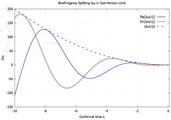
Figure 1. The birefringence effect ($\Delta \omega$) versus conformal time ($\eta$) in the sub-horizon limit. The red line shows the imaginary part, and the blue line shows the real part for the calculated birefringence. The dashed line is the absolute value for $\Delta \omega$, which envelops the real and imaginary parts.

On the other hand, in the super-horizon regime ($\left|k\eta \right|\ll 1$) where the scalar source vanishes, the birefringence splitting is given by

$$\Delta \omega ={\omega }_{+}-{\omega }_{-}\approx i{\displaystyle \frac{14{\vartheta }_0}{l^3}}{e}^{-ik(\eta -z)},$$

(90)

for which the magnitude is independent of $\eta$. This shows that while both helicities are damped by expansion, the relative splitting remains constant in amplitude. In cosmic time, this birefringence survives as a frozen parity-violating imprint in the super-horizon regime as seen in Figure 2.

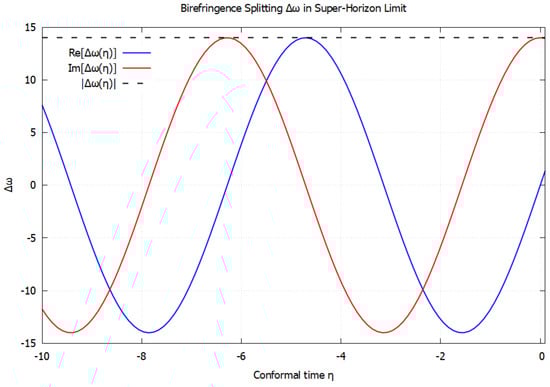
Figure 2. The birefringence effect ($\Delta \omega$) versus conformal time in the super-horizon limit. The red line again shows the imaginary part and the blue the real part, with the dashed line indicating the constant total magnitude.

In the super-horizon regime, the birefringence splitting $\Delta \omega \left(\eta \right)$ approaches a frozen amplitude, as seen from the constant $|\Delta \omega |$. While the real and imaginary parts oscillate with conformal time, their envelope remains bounded, reflecting the fact that Hubble friction damps the overall growth of tensor perturbations. Unlike the sub-horizon case, where birefringence decays away with time, the super-horizon splitting stabilizes to a constant value that is independent of $\eta$. This frozen birefringence imprint persists even as the modes are stretched far beyond the causal horizon, potentially leaving behind a permanent parity-violating signature in the primordial gravitational wave spectrum.

So in the sub-horizon regime, the birefringence rate oscillates with the scalar phase and decays exponentially in cosmic time. Once the super-horizon regime is reached, the birefringence amplitude becomes constant (independent of $\eta$), while both helicities undergo exponential Hubble damping. This distinction highlights that CS-induced parity violation is an early-universe effect that nonetheless may leave persistent imprints on super-horizon tensor modes while becoming negligible for sub-horizon modes at late times.

7. Particular Solution and Flat-Spacetime Limit

In the presence of a scalar background $\vartheta (\eta ,z)$, the inhomogeneous part of the gravitational wave equation admits a nontrivial particular solution. From our analysis [see Equations (64)–(68)], the sub-horizon particular solution (the sourced helicity) takes the form

$$h_{+}^{\left(s\right)\left(\mathrm{part}\right)}(\eta ,z)\approx {\displaystyle \frac{\pi G{\vartheta }_{0}l}{\sqrt{2}{k}^2\eta }}{e}^{-ik(\eta -z)},$$

(91)

while the $h_{-}$ mode has no inhomogeneous source and therefore contains only the homogeneous solution. (Hence, we assume that its sourced amplitude vanishes for the particular-solution flux computation.) The particular solution decays with conformal time as $1/\eta$, reflecting the redshifting of the source in the expanding de Sitter background; it is also suppressed by $1/k^2$, consistent with the intuitive expectation that short-wavelength modes are less efficiently sourced.

7.1. Flux in the Sub-Horizon Regime

The Isaacson energy flux [23,24] along the propagation direction (with $\omega \approx k$) is

$$\mathcal{F}={\displaystyle \frac{{\omega }^2}{32\pi G}}\left[|h_{+}^{\left(s\right)}{|}^2+{|h_{-}^{\left(s\right)}|}^2\right]\approx {\displaystyle \frac{k^2}{32\pi G}}{|h_{+}^{\left(s\right)}|}^2,$$

(92)

where in the last step we have used that the sourced contribution comes only from $h_{+}^{\left(s\right)}$. Using (91) we obtain

$$|h_{+}^{\left(s\right)}{|}^2={\displaystyle \frac{{\pi }^2{G}^2{\vartheta }_0^2{l}^2}{2k^4{\eta }^2}},$$

(93)

so the flux contributed by the particular solution is

$$\mathcal{F}={\displaystyle \frac{k^2}{32\pi G}}{\displaystyle \frac{{\pi }^2{G}^2{\vartheta }_0^2{l}^2}{2k^4{\eta }^2}}={\displaystyle \frac{\pi G}{64}}{\displaystyle \frac{l^2}{k^2{\eta }^2}}{\vartheta }_0^2.$$

(94)

This expression exhibits the expected scalings:

• $\mathcal{F}\propto {\vartheta }_0^2$: There is a quadratic dependence on the scalar amplitude.
• $\mathcal{F}\propto 1/k^2$: Short wavelength modes radiate less efficiently.
• $\mathcal{F}\propto 1/{\eta }^2$: The particular-solution flux grows as conformal time approaches $0^{-}$, equivalently as cosmic time increases (because the sourced amplitude redshifts like $1/\eta$).
• $\mathcal{F}\propto l^2$: The expression has an explicit dependence on the de Sitter radius.

7.2. Flat-Spacetime Limit

The Minkowski (flat-spacetime) limit corresponds to the scale factor approaching unity, $\alpha \left(\eta \right)=\frac{l}{\eta }\to 1$ (equivalently $H\to 0$). It is therefore appropriate to take the limit $\frac{l}{\eta }\to 1$ in the expression for the amplitude rather than setting $\eta =l$ as both may vanish. In this limit the particular-solution amplitude becomes

$$h_{+}^{\left(s\right)\left(\mathrm{part}\right)}{|}_{\alpha \to 1}\approx {\displaystyle \frac{\pi G{\vartheta }_0}{\sqrt{2}{k}^2}}{e}^{-ik(\eta -z)},$$

(95)

and $h_{-}$ remains unsourced. (Only its homogeneous piece survives.) The corresponding flux in the flat limit is given by setting $l/\eta \to 1$ in (94),

$${\mathcal{F}}_{\mathrm{Minkowski}}={\displaystyle \frac{\pi G}{64}}{\displaystyle \frac{1}{k^2}}{\vartheta }_0^2.$$

(96)

Thus, the de Sitter particular-solution result reduces smoothly to the expected Minkowski scaling $\mathcal{F}\propto {\vartheta }_0^2/k^2$ [with the numerical coefficient above determined by our conventions and the $\sqrt{2}$ normalization used in (91)].

7.3. Flux in the Super-Horizon Regime

Outside the horizon, the source vanishes, $S(\eta ,z)=0$, so no net pumping of energy into tensor modes occurs. The tensor modes evolve according to homogeneous evolution and are damped by expansion:

$$h_{\pm }^{\left(s\right)}\sim e^{-Ht}=e^{-t/l},$$

(97)

so the Isaacson flux (which scales as $|{\partial }_t{h|}^2\propto h^2$ for these modes) decays as

$$\mathcal{F}\propto e^{-2Ht}.$$

(98)

At late times the radiated flux therefore vanishes, although a frozen birefringent frequency splitting can remain imprinted in the primordial tensor spectrum. The key point for the present paper is that the sourced radiative flux originates only from the $h_{+}^{\left(s\right)}$ helicity in our setup; the $h_{-}^{\left(s\right)}$ helicity receives no source contribution and only carries whatever homogeneous (unsourced) amplitude was present.

8. Phase Difference Between Helicity States

A key observable manifestation of birefringence is the accumulated phase difference between the right- and left-handed helicity states of the tensor perturbations. It quantifies the relative propagation speed of the two circular polarizations and is defined as

$$\Delta \varphi (k,\eta )={\int }^{\eta }d{\eta }^{\prime }\Re \{\Delta \omega \left({\eta }^{\prime }\right)\},$$

(99)

where $\Delta \omega \left(\eta \right)={\omega }_{+}-{\omega }_{-}$ is the instantaneous frequency splitting between the two helicities. As discussed in Section 6, this splitting is a complex, oscillatory quantity whose real part induces velocity (phase) birefringence, while the imaginary part controls helicity-dependent amplitude modulation.

It is important to specify the lower integration limit in Equation (99). Physically, the phase difference should begin accumulating only after the tensor modes become well-defined, coherent oscillations. For sub-horizon modes ($\left|k\eta \right|\gg 1$), this condition is satisfied in the far past, when the modes behave as free plane waves in the Bunch–Davies vacuum; hence, we choose ${\eta }_{\mathrm{in}}\to -\infty$, ensuring that early-time oscillations contribute a vanishing net phase shift. In contrast, for super-horizon modes ($\left|k\eta \right|\ll 1$), the wave behavior ceases once the mode crosses the horizon. The relevant lower limit is then the horizon-crossing time ${\eta }_{\mathrm{in}}=-1/k$, when the wavelength first equals the Hubble radius. Earlier contributions are exponentially suppressed by Hubble damping and do not affect the observable phase offset. Accordingly, we write

$$\Delta \varphi (k,\eta )={\int }_{{\eta }_{\mathrm{in}}}^{\eta }d{\eta }^{\prime }\Delta \omega \left({\eta }^{\prime }\right),$$

(100)

with ${\eta }_{\mathrm{in}}$ chosen as $-\infty$ for sub-horizon and $-1/k$ for super-horizon analyses.

8.1. Sub-Horizon Regime

Using the dispersion relation (61) valid for $\left|k\eta \right|\gg 1$, the instantaneous frequency splitting is

$$\Re \{\Delta \omega \left(\eta \right)\}=-{\displaystyle \frac{2k{\vartheta }_{0}q}{l^3}}{\eta }^{2}sink(\eta -z).$$

(101)

Integrating gives

$$\Delta {\varphi }_{\mathrm{sub}}(k,\eta )=-{\displaystyle \frac{2k{\vartheta }_{0}q}{l^3}}{\int }_{{\eta }_{\mathrm{in}}}^{\eta }d{\eta }^{\prime }{\eta }^{\prime 2}sink({\eta }^{\prime }-z).$$

(102)

Here ${\eta }_{\mathrm{in}}$ denotes the time when the mode is initialized in the Bunch–Davies vacuum. For calculations one may keep ${\eta }_{\mathrm{in}}$ finite (e.g., when a source turns on) or take the formal limit ${\eta }_{\mathrm{in}}\to -\infty$ with the usual $iϵ$ Tauberian regulator, which suppresses early oscillations.

Carrying out the integration explicitly yields

$$\begin{array}{cc}\hfill I\left(\eta \right)={\int }_{{\eta }_{\mathrm{in}}}^{\eta }d{\eta }^{\prime }{\eta }^{\prime 2}sink({\eta }^{\prime }-z)& =\left(-{\displaystyle \frac{{\eta }^2}{k}}+{\displaystyle \frac{2}{k^3}}\right)cosk(\eta -z)+{\displaystyle \frac{2\eta }{k^2}}sink(\eta -z)+\hfill \\ & \left({\displaystyle \frac{{\eta }_{\mathrm{in}}^2}{k}}-{\displaystyle \frac{2}{k^3}}\right)cosk({\eta }_{\mathrm{in}}-z)-{\displaystyle \frac{2{\eta }_{\mathrm{in}}}{k^2}}sink({\eta }_{\mathrm{in}}-z).\hfill \end{array}$$

(103)

In the limit ${\eta }_{\mathrm{in}}\to -\infty$ the regulated second term vanishes, leaving

$$I\left(\eta \right)=\left(-{\displaystyle \frac{{\eta }^2}{k}}+{\displaystyle \frac{2}{k^3}}\right)cosk(\eta -z)+{\displaystyle \frac{2\eta }{k^2}}sink(\eta -z).$$

(104)

For $\left|k\eta \right|\gg 1$ one may expand the expression as

$$\begin{array}{c}\hfill I\left(\eta \right)={\displaystyle \frac{{\eta }^2}{k}}\left\{-cos\left[k\right(\eta -z\left)\right]+{\displaystyle \frac{2}{k\eta }}sin\left[k\right(\eta -z\left)\right]+{\displaystyle \frac{2}{{\left(k\eta \right)}^2}}cos\left[k\right(\eta -z\left)\right]+\mathcal{O}\left[{\left(k\eta \right)}^{-3}\right]\right\}.\end{array}$$

(105)

The dominant contribution for large $\left|k\eta \right|$ is therefore

$$\Delta {\varphi }_{\mathrm{sub}}(k,\eta ){|}_{\mathrm{leading}}={\displaystyle \frac{2{\vartheta }_{0}q}{l^3}}{\eta }^{2}cos\left[k\right(\eta -z\left)\right],$$

(106)

showing that the envelope of the accumulated phase difference grows as ${\eta }^2$, which corresponds to an exponential decay $\propto e^{-2Ht}$ in cosmic time ($\eta =-e^{-Ht}/H$), since $\left|\eta \right|$ decreases exponentially with t.

8.2. Super-Horizon Regime

In the super-horizon limit ($\left|k\eta \right|\ll 1$), the real part of the frequency splitting between the two helicities is

$$\Re \{\Delta \omega \left(\eta \right)\}={\displaystyle \frac{14{\vartheta }_0}{l^3}}sin\left[k(\eta -z)\right].$$

(107)

The accumulated phase difference, obtained by integrating this real part from the horizon-crossing time ${\eta }_{\mathrm{in}}=-1/k$ to $\eta$, is

$$\Delta {\varphi }_{\mathrm{super}}(k,\eta )={\displaystyle \frac{14{\vartheta }_0}{l^3}}{\displaystyle \frac{1}{k}}\left[cosk({\eta }_{\mathrm{in}}-z)-cosk(\eta -z)\right].$$

(108)

This is the exact expression for the accumulated phase in the super-horizon regime.

For modes well outside the horizon, $\left|k\eta \right|\ll 1$, the cosine terms in Equation (108) may be expanded as

$$cosk(\eta -z)\simeq cos(-kz)\left[1-{\displaystyle \frac{{\left(k\eta \right)}^2}{2}}\right]-sin(-kz)k\eta .$$

(109)

Taking the difference at $\eta$ and ${\eta }_{\mathrm{in}}$ and simplifying gives

$$cosk({\eta }_{\mathrm{in}}-z)-cosk(\eta -z)\simeq {\displaystyle \frac{k^2}{2}}cos\left(kz\right)({\eta }^2-{\eta }_{\mathrm{in}}^2)+ksin\left(kz\right)({\eta }_{\mathrm{in}}-\eta ).$$

(110)

Substituting this into Equation (108) yields

$$\Delta {\varphi }_{\mathrm{super}}(k,\eta )\simeq {\displaystyle \frac{14{\vartheta }_0}{l^3}}\left[{\displaystyle \frac{k}{2}}cos\left(kz\right)({\eta }^2-{\eta }_{\mathrm{in}}^2)+sin\left(kz\right)({\eta }_{\mathrm{in}}-\eta )\right].$$

(111)

The first term in Equation (111) is $\mathcal{O}\left(k\right)$ and thus subleading; the second term dominates for small k. Retaining only the leading-order contribution gives

$$\Delta {\varphi }_{\mathrm{super}}(k,\eta ){|}_{\mathrm{leading}}\approx {\displaystyle \frac{14{\vartheta }_0}{l^3}}sin\left(kz\right)({\eta }_{\mathrm{in}}-\eta ).$$

(112)

With ${\eta }_{\mathrm{in}}=-1/k$, this becomes

$$\Delta {\varphi }_{\mathrm{super}}(k,\eta )\approx -{\displaystyle \frac{14{\vartheta }_0}{k{l}^3}}sin\left(kz\right)-{\displaystyle \frac{14{\vartheta }_0}{l^3}}sin\left(kz\right)\eta .$$

(113)

Since $\left|\eta \right|\ll 1/k$ for super-horizon modes, the $\mathcal{O}(1/k)$ term dominates. The accumulated phase therefore saturates to a constant value after horizon exit, representing a frozen, parity-violating offset imprinted on the tensor modes.

Figure 3 illustrates the phase difference $\Delta \varphi$ between the helicity states of tensor perturbations as a function of conformal time $\eta$ in both the sub-horizon (left) and super-horizon (right) limits. In the sub-horizon regime, the phase difference grows quadratically with $\eta$, reflecting the scaling $\Delta {\varphi }_{\mathrm{sub}}\propto {\eta }^2$. This behavior is consistent with the analytic result that birefringence effects are strongest at early conformal times and decay exponentially in cosmic time as the universe expands. In contrast, the super-horizon regime shows a linear dependence on $\eta$, modulated by oscillatory factors from the scalar background giving rise to a frozen parity-violating phase difference persists once the modes exit the horizon. This distinction highlights how sub- and super-horizon dynamics imprint qualitatively different signatures on the primordial gravitational wave spectrum.

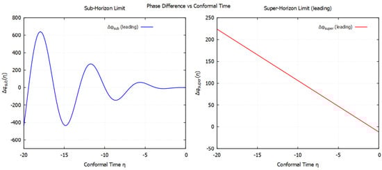
Figure 3. The leading order phase differences ($\Delta \varphi$) versus conformal time for both the sub- and super-horizon limits (in arbitrary units). The plot on left for the sub-horizon limit shows the quadratic dependence ($\propto {\eta }^2$). The plot on right for the super-horizon limit shows the decaying parts as conformal time reaches the far future ($\eta \to 0^{-}$).

9. Amplitude Birefringence

The amplitude ratio $A_{+}/A_{-}$ is another important observable that quantifies the differential amplification or attenuation of the two polarization states of gravitational waves induced by the CS coupling. It is calculated using the expression,

$${\displaystyle \frac{A_{+}}{A_{-}}}=\exp \left[{\int }_{{\eta }_{\mathrm{in}}}^{\eta }d{\eta }^{\prime }\Im \{\Delta \omega \left({\eta }^{\prime }\right)\}\right].$$

(114)

Since the imaginary part of the modified dispersion relation enters the wave amplitude as an exponential factor, integrating $\Im \{\Delta \omega \}$ directly measures the net birefringent amplification accumulated during propagation. This ratio therefore serves as a gauge of amplitude birefringence; a nonzero value signals that parity violation in the CS term has led to unequal damping or enhancement of the left- and right-handed gravitational wave modes. In cosmological settings, this effect provides an observational handle to probe parity-violating interactions in the early universe and can, in principle, imprint a helicity-dependent modulation in the stochastic gravitational wave background [25].

9.1. Sub-Horizon Regime

Inside the sub-horizon regime ($\left|k\eta \right|\gg 1$), the CS modification introduces a small imaginary component to the frequency of each helicity mode. From Equations (61)–(63), the imaginary parts of the two helicity branches are

$$\Im \left\{{\omega }_{\pm }\right\}=\mp {\displaystyle \frac{k{\vartheta }_{0}q}{{\alpha }^{2}l}}cos\left[k\right(\eta -z\left)\right],$$

(115)

where ${\vartheta }_0$ characterizes the CS coupling amplitude, and $\alpha \left(\eta \right)=l/\eta$ for the de Sitter background. The imaginary part of the helicity frequency splitting $\Delta \omega \equiv {\omega }_{+}-{\omega }_{-}$ is then

$$\Im \{\Delta \omega \}=\Im \left\{{\omega }_{+}\right\}-\Im \left\{{\omega }_{-}\right\}=-{\displaystyle \frac{2k{\vartheta }_{0}q{\eta }^2}{l^3}}cos\left[k\right(\eta -z\left)\right].$$

(116)

The relative amplitude of the two helicity states follows from integrating the imaginary frequency difference. To evaluate the exponent, define

$$I^{\prime }\left(\eta \right)\equiv {\int }^{\eta }d{\eta }^{\prime }{\eta }^{\prime 2}cos\left[k({\eta }^{\prime }-z)\right].$$

(117)

An explicit anti-derivative is given as

$$I^{\prime }\left(\eta \right)={\displaystyle \frac{{\eta }^2{k}^{2}sin\left[k(\eta -z)\right]+2\eta kcos\left[k(\eta -z)\right]-2sin\left[k(\eta -z)\right]}{k^3}}+\mathrm{const}.$$

(118)

Substituting this into Equation (115), we obtain the exact sub-horizon expression

$$\begin{array}{ccc}\hfill ln{\displaystyle \frac{A_{+}}{A_{-}}}& =& -{\displaystyle \frac{2k{\vartheta }_{0}q}{l^3}}\{{\displaystyle \frac{{\eta }^2{k}^{2}sin\left[k(\eta -z)\right]+2\eta kcos\left[k(\eta -z)\right]-2sin\left[k(\eta -z)\right]}{k^3}}\hfill \\ & & -{\displaystyle \frac{{\eta }_{\mathrm{in}}^2{k}^{2}sin\left[k({\eta }_{\mathrm{in}}-z)\right]+2{\eta }_{\mathrm{in}}kcos\left[k({\eta }_{\mathrm{in}}-z)\right]-2sin\left[k({\eta }_{\mathrm{in}}-z)\right]}{k^3}}\}.\hfill \end{array}$$

(119)

In the deep sub-horizon limit, for a Bunch–Davies initialization in the remote past (${\eta }_{\mathrm{in}}\to -\infty$) the oscillatory boundary term averages out, leaving the leading behavior

$$ln{\displaystyle \frac{A_{+}}{A_{-}}}\simeq -{\displaystyle \frac{2{\vartheta }_{0}q}{l^3}}{\eta }^{2}sin\left[k\right(\eta -z\left)\right],$$

(120)

for $\left|k\eta \right|\gg 1$ Thus, the helicity amplitude ratio oscillates with the phase of the CS background, and its envelope scales as ${\eta }^2$ in conformal time. Since $\eta =-e^{-Ht}/H$ in de Sitter space, this corresponds to an exponentially decaying envelope $\propto e^{-2Ht}$ in cosmic time. The periodic sign change of the sine term indicates alternating amplification and attenuation of opposite helicities as the gravitational wave propagates through successive CS phase regions.

9.2. Super-Horizon Regime

In the super-horizon regime ($\left|k\eta \right|\ll 1$), the imaginary part of the frequency splitting $\Delta \omega$ is given by the following:

$$\Im \{\Delta \omega \}={\displaystyle \frac{14{\vartheta }_0}{l^3}}cos\left[k\right(\eta -z\left)\right].$$

(121)

Integrating over conformal time we obtain the relation

$$ln{\displaystyle \frac{A_{+}}{A_{-}}}={\displaystyle \frac{14{\vartheta }_0}{l^{3}k}}\left\{sin\left[k\right(\eta -z\left)\right]-sin\left[k({\eta }_{\mathrm{in}}-z)\right]\right\}$$

(122)

In the limit of $\left|k\eta \right|\ll 1$, we can use the Taylor expansion,

$$sin\left[k(\eta -z)\right]=sin(-kz)+k\eta cos(-kz)-\frac{1}{2}{\left(k\eta \right)}^{2}sin(-kz)+\mathcal{O}\left[{\left(k\eta \right)}^3\right].$$

(123)

Equation (122) becomes

$$\begin{array}{ccc}\hfill ln{\displaystyle \frac{A_{+}}{A_{-}}}& =& {\displaystyle \frac{14{\vartheta }_0}{l^{3}k}}\left\{sin(-kz)-sin\left[k({\eta }_{\mathrm{in}}-z)\right]\right\}+{\displaystyle \frac{14{\vartheta }_0}{l^3}}\eta cos(-kz)\hfill \\ & & -{\displaystyle \frac{7{\vartheta }_0}{l^3}}k{\eta }^{2}sin(-kz)+\mathcal{O}\left[{\left(k\eta \right)}^2\right].\hfill \end{array}$$

(124)

The leading term (in French brackets) is independent of $\eta$ and represents a frozen amplitude asymmetry established when the mode exits the horizon. The next term, linear in $\eta$, describes a small residual time dependence suppressed by $k\eta$ and therefore negligible deep in the super-horizon regime.

The physical interpretation is that on super-horizon scales, the amplitude birefringence effectively freezes out; the differential amplification of the two helicities reaches a constant value once $\left|k\eta \right|\ll 1$. This behavior reflects the fact that outside the horizon, tensor modes evolve as nearly constant background distortions, and further parity-violating amplification is exponentially suppressed by cosmic expansion.

Figure 4 illustrates the logarithm of the helicity amplitude ratio $ln(A_{+}/A_{-})$ as a function of conformal time $\eta$ for both the sub-horizon and super-horizon limits. In the sub-horizon regime, the amplitude ratio exhibits an oscillatory behavior whose envelope grows as ${\eta }^2$, reflecting the alternating amplification and attenuation of opposite helicities as they propagate through the CS background. In contrast, the super-horizon behavior approaches a nearly constant value with only a small $\eta$-linear correction, corresponding to the freezing of amplitude birefringence once the mode exits the horizon. The constant offset and the weak slope arise from the residual imaginary part of the frequency splitting, consistent with the analytic expression derived in Equation (124). This figure thus highlights the qualitative difference between the dynamic sub-horizon amplification and the frozen super-horizon asymmetry of gravitational-wave amplitudes in a parity-violating background.

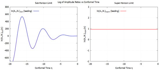
Figure 4. The ratio of the log of amplitudes in the leading order, $ln\left(A_{+}/A_{-}\right)$ versus conformal time ($\eta$) for both the sub- and super-horizon limits. The plot on left for the sub-horizon limit shows the quadratic dependence ($\propto {\eta }^2$) and enveloped by an oscillatory term. The plot on right for the super-horizon limit shows the constant frozen-in amplitude difference that remains etched in the distant future ($\eta \to 0^{-}$).

10. Dark Matter Relations and Modifications

The preceding analysis has treated the CS field $\vartheta$ as a massless scalar. However, from a phenomenological standpoint, it is compelling to consider that $\vartheta$ may itself constitute the dark matter, or a significant portion of it. Well-motivated candidates for dark matter, such as axions or axion-like particles (ALPs), are light pseudoscalar fields, and the curvature coupling for $\vartheta$ has the same discrete symmetries as an ALP coupling. In this section, we promote $\vartheta$ to a massive field and analyze how its identity as a dark matter component modifies the gravitational birefringence effects calculated in the massless case.

Building on this idea, it was demonstrated that generalized gravity theories, including scalar-tensor and string-inspired models, yield distinctive gravitational-wave spectra (typically with a blue tilt, $n_T\simeq 3$) during pole-like inflation, differing fundamentally from the scale-invariant case in Einstein gravity [26]. It was also shown that the string-theoretic axion coupling to ${}^{\star }\mathcal{RR}$ induces parity-violating, polarization-dependent evolution of tensor perturbations, leading to potentially observable gravitational-wave birefringence imprinted in the CMB [27].

10.1. Massive Chern–Simons Dark Matter Field

We now consider a massive scalar field with a potential:

$$V\left(\vartheta \right)={\displaystyle \frac{1}{2}}{m}^2{\vartheta }^2,$$

(125)

where m is the mass of the dark matter particle. The action from Equation (1) remains unchanged, but the equation of motion for the $\vartheta$ field (4) gains a mass term:

$$\square \vartheta -m^2\vartheta =-{\displaystyle \frac{1}{4}}{(}^{\star }\mathcal{RR}).$$

(126)

For the homogeneous background field in a de Sitter universe, and neglecting the Pontryagin density source term at zeroth order, this equation becomes

$${\vartheta }^{″}+2{\displaystyle \frac{{\alpha }^{\prime }}{\alpha }}{\vartheta }^{\prime }+m^2{\alpha }^2\vartheta =0,$$

(127)

which is another parametric oscillator equation. Substituting the scale factor $\alpha =l/\eta$ yields

$${\vartheta }^{″}-{\displaystyle \frac{2}{\eta }}{\vartheta }^{\prime }+{\displaystyle \frac{m^2{l}^2}{{\eta }^2}}\vartheta =0.$$

(128)

The general solution to this equation is a linear combination of Hankel functions,

$$\vartheta \left(\eta \right)={(-\eta )}^{3/2}\left[C_1{H}_{\nu }^{\left(1\right)}(-k\eta )+C_2{H}_{\nu }^{\left(2\right)}(-k\eta )\right],$$

(129)

where

$$\nu =\sqrt{{\displaystyle \frac{9}{4}}-{\left(ml\right)}^2}.$$

(130)

The Bunch–Davies vacuum condition selects $C_2=0$. The key difference from the massless case is the order of the Hankel function, $\nu$, which now depends on the product $ml$.

10.2. Modifications in the Sub-Horizon Limit

The mass term introduces a new scale that competes with the Hubble parameter. The behavior of the field, and consequently all derived quantities, changes significantly.

In the sub-horizon limit, the asymptotic form of the solution is a modulated plane wave. However, the functional form of the amplitude is more complicated than the simple $\eta /l$ decay of the massless case. The solution can be approximated as

$${\vartheta }_k\left(\eta \right)\approx {\vartheta }_0\mathcal{F}(ml,k\eta )e^{-ik\eta },$$

(131)

where $\mathcal{F}(ml,k\eta )$ is a function that reduces to $\eta /l$ for $m=0$ but deviates from this simple form for $m>0$. This altered time dependence propagates into the coefficients that define the Cotton tensor and the source term. The derivatives $v_{\mu }={\nabla }_{\mu }\vartheta$ become

$$\begin{array}{ccc}\hfill v_{\eta }& =& {\partial }_{\eta }\vartheta \approx {\vartheta }_0({\partial }_{\eta }\mathcal{F}-ik\mathcal{F})e^{-ik\eta }\hfill \end{array}$$

(132)

$$\begin{array}{ccc}\hfill v_z& =& {\partial }_z\vartheta \approx {\vartheta }_0\left(ik\mathcal{F}\right)e^{-ik\eta }.\hfill \end{array}$$

(133)

The second derivatives ($v_{\eta \eta }$, $v_{\eta z}$, and $v_{zz}$) are modified similarly. This means the Cotton tensor prefactor $f(\omega ,q,k,\eta )$ from (56) is no longer a simple polynomial in $\eta$ but a more complex function

$$f(\omega ,q,k,\eta )\to {\displaystyle \frac{{\vartheta }_0}{l}}\tilde{f}(ml,\omega ,q,k,\eta ).$$

(134)

The dispersion relation correction in the sub-horizon regime is consequently modified. The frequency splitting between helicities will become

$$\Delta \omega ={\omega }_{+}-{\omega }_{-}\approx {\displaystyle \frac{2}{{\alpha }^2}}\left|\tilde{f}(ml,q,q,k,\eta )\right|.$$

(135)

The explicit time dependence $\Delta \omega \propto {\eta }^2$ is replaced by a mass-dependent function $\tilde{f}$. The strength of the birefringence effect in the early universe now explicitly depends on the dark matter mass m. For a very light field ($m\ll H$), we recover the massless result. For a heavier field, the effect can be either suppressed or enhanced, providing a potential observational link between the parity-violating imprint on primordial gravitational waves and the mass of the dark matter particle.

The particular solution for the sourced gravitational waves is also altered. The source term $S(\eta ,z)$ scales as ${(\nabla \vartheta )}^2$. Its new functional form is

$$S(\eta ,z)\propto {\displaystyle \frac{{\vartheta }_0^2}{l^2}}{\left|\mathcal{F}(ml,k\eta )\right|}^2.$$

(136)

Following the same analysis the amplitude of the particular solution becomes

$$h_{\pm }^{\left(\mathrm{part}\right)}\propto \pm {\displaystyle \frac{\pi G{\vartheta }_{0}l}{k^2\eta }}{\left|\mathcal{F}(ml,k\eta )\right|}^2.$$

(137)

This result indicates that the efficiency of gravitational wave production by the CS dark matter field is mass dependent. A field with some specific mass could potentially be a more efficient generator of primordial gravitational waves than a massless one.

10.3. Late-Time Behavior And Consistency

A crucial feature of this model is its consistency with the standard cosmological model at late times. In the frozen regime ($H\gg m)$, $\vartheta$ is nearly constant and maximally sources parity-violating birefringence. When the Hubble parameter drops below the mass scale ($H<m$), the field $\vartheta$ begins to oscillate, and its energy density redshifts as pressureless dust, ${\rho }_{\vartheta }\propto a^{-3}$, behaving as standard cold dark matter [28,29,30]. Furthermore, the amplitude of oscillation decays as $⟨\vartheta ⟩\propto a^{-3/2}$. Since the CS effects are driven by derivatives of $\vartheta$, they become exponentially suppressed at late times. This ensures that the intense parity-violating effects are confined to the early universe, evading constraints from solar system tests, binary pulsar observations, and direct gravitational wave detections by LIGO/Virgo/KAGRA [31].

The model leaves behind a permanent, frozen record of this early-era physics in the form of a chiral, blue-tilted primordial gravitational wave spectrum, without affecting late-time gravity. This connects naturally with studies of parity violation in the early universe and its possible observational imprints on the CMB and stochastic gravitational wave background [32]. In this way, the birefringence scaling can act as a probe of the dark matter mass, interpolating smoothly between the massless axion-like case and the standard cold dark matter regime.

Promoting the CS field $\vartheta$ to a massive dark matter candidate introduces a potentially rich layer of phenomenology. The simple, power-law time dependencies found in the massless case are replaced by more complex, mass-dependent functions. This establishes a direct theoretical link between the properties of dark matter (its mass m) and the characteristics of primordial gravitational birefringence and wave generation. This model could provide a compelling framework for seeking dark matter signatures in the polarization of the cosmic microwave background and the stochastic gravitational wave background, and this connection will be examined in future work.

11. Conclusions

In this work, we have carried out a detailed analysis of tensor perturbations in de Sitter spacetime within the framework of CS modified gravity. Beginning from the conformally flat form of the metric, we computed the curvature tensors and perturbed field equations, showing explicitly that the Pontryagin density vanishes at linear order while the Cotton tensor introduces parity-violating corrections to gravitational wave propagation. The decoupled helicity modes reveal birefringence in both sub- and super-horizon regimes: oscillatory and exponentially suppressed inside the horizon, but frozen to a constant splitting once the modes cross the horizon. We also derived particular solutions sourced by the scalar background, demonstrating the amplification of one helicity due to the CS coupling, together with explicit expressions for the radiated flux and its smooth reduction to the flat-space limit.

A key observable studied here is the accumulated phase difference between right- and left-handed tensor modes. We showed that in the sub-horizon limit, this phase difference grows quadratically with conformal time, whereas in the super-horizon regime it approaches a frozen value that survives as a persistent parity-violating imprint in the primordial tensor spectrum. This provides a clear physical mechanism for how CS modifications can be encoded in the polarization of relic gravitational waves, which is consistent with earlier suggestions that such parity-violating effects could leave observable imprints on the CMB and stochastic backgrounds. Notably, the birefringence effect exhibits a continuous transition from amplitude modulation to velocity (phase) birefringence as the scalar field phase evolves, indicating that the dominant observable shifts from differential damping to differential propagation speed depending on the relative phase between the gravitational and scalar fields.

Finally, we extended the analysis by promoting the CS scalar to a massive dark matter candidate. The introduction of a mass modifies both the time dependence of the background field and the efficiency of gravitational wave sourcing, leading to a direct link between dark matter phenomenology and parity-violating gravitational imprints. Importantly, the CS effects are naturally suppressed at late times, ensuring consistency with astrophysical and gravitational wave constraints, while leaving unique signatures in the early universe.

In summary, our results demonstrate that Chern–Simons modified gravity in a de Sitter background produces distinctive birefringence and phase-shift signatures in primordial tensor modes, which are potentially accessible to future cosmic microwave background polarization measurements and gravitational wave observatories. Future work should address higher-order effects, nonlinear backreaction, and realistic reheating scenarios to refine these predictions and strengthen the observational connection between parity-violating gravity and early-universe cosmology.

Appendix C.1. Time–Time Cotton Tensor

Using the fact that ${\overline{C}}_{\eta \eta }=0$, we can find the perturbation in the time–time Cotton tensor comnponent,

$$\delta C_{\eta \eta }=-\left[v_{\alpha }\left({ϵ}^{\alpha \beta \sigma \tau }{\overline{g}}_{\eta \beta }{\nabla }_{\sigma }\delta R_{\eta \tau }\right)+{\displaystyle \frac{1}{2}}{v}_{\sigma \tau }\left({\overline{g}}_{\eta \gamma }{ϵ}^{\sigma \gamma \alpha \beta }\delta {R^{\tau }}_{\eta \alpha \beta }\right)\right].$$

(A75)

For the first term on the right-hand side, we can see that the term will exist only when $\beta =\eta$ and also $\tau =\eta$; however, if both of these indices are taken to be $\eta$ then the Levi–Civita symbol vanishes. So the first does not contribute. For the second term on the right-hand side, we see that $\gamma =\eta$, which makes all the other indices $\sigma ,\alpha$, and $\beta$ spatial. Therefore, the expression becomes

$$\delta C_{\eta \eta }=-{\displaystyle \frac{1}{2}}{v}_{m\tau }{\overline{g}}_{\eta \gamma }{ϵ}^{m\gamma ij}\delta {R^{\tau }}_{\eta ij}.$$

(A76)

The Riemann tensor has the summable index $\tau$ which can take either of the values $\eta$ or a spatial index. When we substitute $\tau =\eta$ the Riemann tensor ${R^{\eta }}_{\eta ij}$ vanishes. So the only potentially existent term that remains is

$$\begin{array}{ccc}\hfill \delta C_{\eta \eta }& =& -{\displaystyle \frac{1}{2}}{v}_{mk}{\overline{g}}_{\eta \gamma }{ϵ}^{m\gamma ij}\delta {R^k}_{\eta ij}\hfill \end{array}$$

(A77)

$$\begin{array}{ccc}& =& -{\displaystyle \frac{1}{4}}{v}_{mk}{\overline{g}}_{\eta \gamma }{ϵ}^{m\gamma ij}\left({\partial }_i{\partial }_{\eta }{\gamma }_j^k-{\partial }_j{\partial }_{\eta }{\gamma }_i^k\right),\hfill \end{array}$$

(A78)

which also vanished because of the TT condition. So the final expression for the time–time Cotton tensor component is

$$\delta C_{\eta \eta }=0.$$

(A79)

Appendix C.2. Mixed Cotton Tensor

For the mixed time-space components in the perturbed metric, we again calculate the two parts, starting with

$$\delta C_{\eta i}^{\left(1\right)}=-{\displaystyle \frac{1}{2}}\left[v_{\alpha }\left({ϵ}^{\alpha \beta \sigma \tau }{\overline{g}}_{\eta \beta }{\nabla }_{\sigma }\delta R_{i\tau }+{ϵ}^{\alpha \gamma \sigma \tau }{\overline{g}}_{i\gamma }{\nabla }_{\sigma }\delta R_{\eta \tau }\right)\right].$$

(A80)

The second term on the right-hand side demands that $\tau =\eta$, and that also means that $\sigma =\eta$, since as $R_{\eta \eta }$ is a function of $\eta$ only. That makes the Levi–Civita symbol become zero; hence the second term makes no contribution. For the first term to exist, the only nonzero contribution will come if $\tau =j$, leaving the components to take the form

$$\begin{array}{ccc}\hfill \delta C_{\eta i}^{\left(1\right)}& =& -{\displaystyle \frac{1}{2}}{v}_{\alpha }\left({ϵ}^{\alpha \beta \sigma j}{\overline{g}}_{\eta \beta }{\nabla }_{\sigma }\delta R_{ij}\right)\hfill \end{array}$$

(A81)

$$\begin{array}{ccc}& =& -{\displaystyle \frac{{\alpha }^2}{2}}{v}_{\alpha }\left({ϵ}^{\alpha \beta \sigma j}{\delta }_{\eta \beta }{\nabla }_{\sigma }\delta R_{ij}\right).\hfill \end{array}$$

(A82)

Since $\beta$ has to be replaced by $\eta$ as demanded by ${\delta }_{\eta \beta }$, this implies $\alpha$ and $\sigma$ have to be spatial indices, and we know that $\alpha$ has to be z for this to exist. Hence, the relation takes the form

$$\delta C_{\eta i}^{\left(1\right)}={\displaystyle \frac{{\alpha }^2}{2}}{v}_z\left({\delta }_{\eta \beta }{ϵ}^{z\beta kj}{\nabla }_k\delta R_{ij}\right).$$

(A83)

Again, for this to exist k has to be z, and that leads to two repeated indices in the Levi–Civita symbol, which thus vanishes. Hence, we find that the first part of the perturbation in the mixed Cotton tensor vanishes. For the second part of the perturbed Cotton tensor we have the expression

$$C_{\eta i}^{\left(2\right)}=-{\displaystyle \frac{1}{4}}{v}_{\sigma \tau }\left[{\overline{g}}_{i\gamma }{ϵ}^{\sigma \gamma \alpha \beta }\delta {R^{\tau }}_{\eta \alpha \beta }+{\overline{g}}_{\eta \rho }{ϵ}^{\sigma \rho \alpha \beta }\delta {R^{\tau }}_{i\alpha \beta }\right].$$

(A84)

Using the sets of indices for $\sigma$ and $\tau$ that are possible, we see that this second part also vanishes. Hence, we obtain another three vanishing tensor components,

$$\delta C_{\eta i}=0.$$

(A85)

Appendix C.3. Spatial Cotton Tensor

Things become more complicated with the space-space terms in the Cotton tensor. The background Cotton tensor for the unperturbed de Sitter spacetime was calculated to vanish. Therefore, the only contribution will be from the perturbation part of the metric. However, unlike $\delta C_{\eta \eta }$ and $\delta C_{\eta i}$, we need not have $\delta C_{ij}$ be zero. We can see in the first term on the right-hand side of Equation (A74) with $\mu =i$ and $\nu =j$ that the only existent perturbation in the Ricci tensor occurs when we have $\tau$ as another spatial index. No other Ricci tensor terms have any perturbation. Using this we obtain

$$\delta C_{ij}^{\left(1\right)}=-{\displaystyle \frac{1}{2}}\left[v_{\alpha }\left({ϵ}^{\alpha \beta \sigma k}{\overline{g}}_{i\beta }{\nabla }_{\sigma }\delta R_{jk}+{ϵ}^{\alpha \gamma \sigma k}{\overline{g}}_{j\gamma }{\nabla }_{\sigma }\delta R_{ik}\right)\right].$$

(A86)

There can be two possible sets of indices that keep the Levi–Civita symbol intact: $\alpha =\eta$ and $\sigma =z$, or $\alpha =z$ and $\sigma =\eta$. Combining those two, we obtain

$$\delta C_{ij}^{\left(1\right)}=-{\displaystyle \frac{1}{2}}\left(v_{\eta }{\nabla }_z-v_z{\nabla }_{\eta }\right)\left({\overline{g}}_{i\rho }{ϵ}^{\eta \rho zk}\delta R_{jk}+{\overline{g}}_{j\gamma }{ϵ}^{\eta \gamma zk}\delta R_{ik}\right).$$

(A87)

We also calculate the expression for the second part of the perturbed Cotton tensor,

$$\delta C_{ij}^{\left(2\right)}=-{\displaystyle \frac{1}{4}}\left[v_{\sigma \tau }\left({\overline{g}}_{j\gamma }{ϵ}^{\sigma \gamma \alpha \beta }\delta {R^{\tau }}_{i\alpha \beta }+{\overline{g}}_{i\rho }{ϵ}^{\sigma \rho \alpha \beta }\delta {R^{\tau }}_{j\alpha \beta }\right)\right].$$

(A88)

We see that there can be four sets of index choices for $\sigma$ and $\tau$ which make these terms to be nonzero. Using all four, we obtain an expression for the perturbation,

$$\begin{array}{ccc}\hfill \delta C_{ij}^{\left(2\right)}& =& -{\displaystyle \frac{1}{2}}\left[{\overline{g}}_{i\rho }{ϵ}^{\eta \rho zk}\left(v_{\eta \eta }\delta {R^{\eta }}_{jzk}+v_{\eta z}\delta {R^z}_{jzk}+v_{z\eta }\delta {R^{\eta }}_{j\eta k}+v_{zz}\delta {R^z}_{j\eta k}\right)\right]\hfill \\ & & -{\displaystyle \frac{1}{2}}\left[{\overline{g}}_{j\gamma }{ϵ}^{\eta \gamma zk}\left(v_{\eta \eta }\delta {R^{\eta }}_{izk}+v_{\eta z}\delta {R^z}_{izk}+v_{z\eta }\delta {R^{\eta }}_{i\eta k}+v_{zz}\delta {R^z}_{i\eta k}\right)\right].\hfill \end{array}$$

(A89)

The point to note here is that both the perturbations in the Cotton tensor vanish when we choose either of the indices i or j to be the direction of propagation (the z-direction). So the only existing Cotton tensor perturbations can be in the $xx$, $xy$, or $yy$ components, thus mirroring the form of the perturbation introduced into the metric.

Appendix C.4. Non-Vanishing Cotton Tensor Elements

We will conclude this appendix by calculating the three specific, nonzero Cotton tensor elements. We start with the $xx$ component,

$$C_{xx}^{\left(1\right)}=-\left(v_{\eta }{\nabla }_z-v_z{\nabla }_{\eta }\right)\left({\overline{g}}_{x\rho }{ϵ}^{\eta \rho zk}\delta R_{xk}\right).$$

(A90)

Using the facts that ${\overline{g}}_{x\rho }={\alpha }^2{\delta }_{x\rho }$ and ${ϵ}^{\eta \rho zk}={\displaystyle \frac{{\epsilon }^{\eta \rho zk}}{\sqrt{-g}}}$, we obtain

$$\begin{array}{ccc}\hfill C_{xx}^{\left(1\right)}& =& -{\displaystyle \frac{1}{\sqrt{-g}}}\left(v_{\eta }{\nabla }_z-v_z{\nabla }_{\eta }\right)\left({\alpha }^2{\delta }_{x\rho }{\epsilon }^{\eta \rho zk}\delta R_{xk}\right)\hfill \end{array}$$

(A91)

$$\begin{array}{ccc}& =& -{\displaystyle \frac{1}{\sqrt{-g}}}\left(v_{\eta }{\nabla }_z-v_z{\nabla }_{\eta }\right)\left({\alpha }^2{\delta }_{x\rho }{\epsilon }^{\eta \rho zy}\delta R_{xy}\right)\hfill \end{array}$$

(A92)

$$\begin{array}{ccc}& =& {\displaystyle \frac{1}{\sqrt{-g}}}\left(v_{\eta }{\nabla }_z-v_z{\nabla }_{\eta }\right)\left({\alpha }^2\delta R_{xy}\right)\hfill \end{array}$$

(A93)

$$\begin{array}{ccc}& =& v_{\eta }\left[{\nabla }_z\left({\displaystyle \frac{1}{{\alpha }^2}}\delta R_{xy}\right)\right]-v_z\left[{\nabla }_{\eta }\left({\displaystyle \frac{1}{{\alpha }^2}}\delta R_{xy}\right)\right].\hfill \end{array}$$

(A94)

Now the covariant derivative can be calculated as

$${\nabla }_z\left({\displaystyle \frac{1}{{\alpha }^2}}\delta R_{xy}\right)={\displaystyle \frac{1}{{\alpha }^2}}\left({\partial }_z\delta R_{xy}-{\Gamma }_{zy}^{\lambda }\delta R_{x\lambda }-{\Gamma }_{zx}^{\lambda }\delta R_{\lambda y}\right).$$

(A95)

The Christoffel symbols are first order in ${\gamma }_{ij}$ and hence, in the linearized theory, their contractions with $\delta R_{ij}$ may be neglected. So, the covariant derivative simplifies to

$${\nabla }_z\left({\displaystyle \frac{1}{{\alpha }^2}}\delta R_{xy}\right)={\displaystyle \frac{1}{{\alpha }^2}}\left({\partial }_z\delta R_{xy}\right).$$

(A96)

Similarly, for the other term in Equation (A94), we have

$${\nabla }_{\eta }\left(\delta R_{xy}\right)={\partial }_{\eta }\delta R_{xy}.-{\Gamma }_{\eta y}^{\lambda }\delta R_{x\lambda }-{\Gamma }_{\eta x}^{\lambda }\delta R_{\lambda y}$$

(A97)

Using the form of the Christoffel symbol ${\Gamma }_{\eta j}^i$, we can see the background contribution (which is nonzero in this term),

$${\nabla }_{\eta }\left(\delta R_{xy}\right)={\partial }_{\eta }\delta R_{xy}+{\displaystyle \frac{2}{\eta }}\delta R_{xy}.$$

(A98)

From this, we find

$$\begin{array}{ccc}\hfill {\nabla }_{\eta }\left({\displaystyle \frac{1}{{\alpha }^2}}\delta R_{xy}\right)& =& {\displaystyle \frac{1}{{\alpha }^2}}{\nabla }_{\eta }\delta R_{xy}+{\partial }_{\eta }\left({\displaystyle \frac{1}{{\alpha }^2}}\right)\delta R_{xy}\hfill \end{array}$$

(A99)

$$\begin{array}{ccc}& =& {\displaystyle \frac{1}{{\alpha }^2}}{\partial }_{\eta }\delta R_{xy}+\left({\displaystyle \frac{2}{\eta {\alpha }^2}}\right)\delta R_{xy}-{\displaystyle \frac{2{\alpha }^{\prime }}{{\alpha }^3}}\delta R_{xy}\hfill \end{array}$$

(A100)

$$\begin{array}{ccc}& =& {\displaystyle \frac{1}{{\alpha }^2}}\left({\partial }_{\eta }\delta R_{xy}+{\displaystyle \frac{4}{\eta }}\delta R_{xy}\right).\hfill \end{array}$$

(A101)

So the first part of the Cotton tensor becomes

$$C_{xx}^{\left(1\right)}={\displaystyle \frac{1}{{\alpha }^2}}\left({\displaystyle \frac{v_{\eta }}{2}}{\partial }_z\delta R_{xy}-{\displaystyle \frac{v_z}{2}}{\partial }_{\eta }\delta R_{xy}-{\displaystyle \frac{4v_z}{\eta }}\delta R_{xy}\right).$$

(A102)

In a similar fashion, for the second part we obtain

$$C_{xx}^{\left(2\right)}={\displaystyle \frac{1}{\sqrt{-g}}}\left[{\alpha }^2{\delta }_{x\rho }{\epsilon }^{\eta \rho zk}\left(v_{\eta \eta }{R^{\eta }}_{xzk}+v_{\eta z}{R^z}_{xzk}+v_{z\eta }{R^{\eta }}_{x\eta k}+v_{zz}{R^z}_{x\eta k}\right)\right].$$

(A103)

Using the Riemann tensor components and the fact that k can only be y, we find

$$C_{xx}^{\left(2\right)}={\displaystyle \frac{1}{{\alpha }^2}}\left[v_{\eta \eta }\left({\displaystyle \frac{1}{2}}{\partial }_z{\partial }_{\eta }{\gamma }_{xy}\right)+v_{\eta z}\left({\displaystyle \frac{1}{2}}\square {\gamma }_{xy}\right)+v_{zz}\left(-{\displaystyle \frac{1}{2}}{\partial }_{\eta }{\partial }^z{\gamma }_{xy}\right)\right].$$

(A104)

So, the $xx$ component of Cotton tensor takes the final form

$$\begin{array}{ccc}\hfill C_{xx}& =& {\displaystyle \frac{1}{{\alpha }^2}}[{\displaystyle \frac{v_{\eta }}{2}}{\partial }_z\square {\gamma }_{xy}-{\displaystyle \frac{v_z}{2}}{\partial }_{\eta }\square {\gamma }_{xy}-{\displaystyle \frac{4v_z}{\eta }}\square {\gamma }_{xy}\hfill \\ & & +v_{\eta \eta }\left({\displaystyle \frac{1}{2}}{\partial }_z{\partial }_{\eta }{\gamma }_{xy}\right)+v_{\eta z}\left({\displaystyle \frac{1}{2}}\square {\gamma }_{xy}\right)+v_{zz}\left(-{\displaystyle \frac{1}{2}}{\partial }_{\eta }{\partial }^z{\gamma }_{xy}\right)],\hfill \end{array}$$

(A105)

where we have used $\square =({\partial }_{\eta }^2+2{\displaystyle \frac{{\alpha }^{\prime }}{\alpha }}{\partial }_{\eta }-{\partial }_z^2)$.

To obtain the $yy$ component, we only need to note the facts that ${\gamma }_{yy}=-{\gamma }_{xx}$ and ${\gamma }_{xy}={\gamma }_{yx}$. From these follow the relation

$$C_{yy}=-C_{xx}.$$

(A106)

Finally, for the $xy$ cross term in Cotton tensor we obtain

$$\begin{array}{ccc}\hfill C_{xy}^{\left(1\right)}& =& {\displaystyle \frac{1}{{\alpha }^2}}\left[{\displaystyle \frac{v_{\eta }}{2}}{\partial }_z\square {\gamma }_{xx}-{\displaystyle \frac{v_z}{2}}{\partial }_{\eta }\square {\gamma }_{xx}-{\displaystyle \frac{4v_z}{\eta }}\square {\gamma }_{xx}\right]\hfill \end{array}$$

(A107)

$$\begin{array}{ccc}\hfill C_{xy}^{\left(2\right)}& =& {\displaystyle \frac{1}{{\alpha }^2}}\left[v_{\eta \eta }\left({\displaystyle \frac{1}{2}}{\partial }_z{\partial }_{\eta }{\gamma }_{xx}\right)+v_{\eta z}\left({\displaystyle \frac{1}{2}}\square {\gamma }_{xx}\right)+v_{zz}\left(-{\displaystyle \frac{1}{2}}{\partial }_{\eta }{\partial }^z{\gamma }_{xx}\right)\right].\hfill \end{array}$$

(A108)

References

- de Sitter, W. On the relativity of inertia. Remarks concerning Einstein’s latest hypothesis. Proc. R. Neth. Acad. Arts Sci. 1917, 19, 1217. [Google Scholar]
- Hawking, S.W. The unpredictability of quantum gravity. Commun. Math. Phys. 1975, 43, 199. [Google Scholar] [CrossRef]
- Mukhanov, V. Physical Foundations of Cosmology; Cambridge University Press: Cambridge, UK, 2005. [Google Scholar]
- Guth, A.H. Inflationary universe: A possible solution to the horizon and flatness problems. Phys. Rev. D 1981, 23, 347. [Google Scholar] [CrossRef]
- Linde, A.D. A new inflationary universe scenario: A possible solution of the horizon, flatness, homogeneity, isotropy and primordial monopole problems. Phys. Lett. B 1982, 108, 389. [Google Scholar] [CrossRef]
- Albrecht, A.; Steinhardt, P.J. Cosmology for grand unified theories with radiatively induced symmetry breaking. Phys. Rev. Lett. 1982, 48, 1220. [Google Scholar] [CrossRef]
- Mukhanov, V.; Chibisov, G. Quantum fluctuations and a nonsingular universe. JETP Lett. 1981, 33, 532. [Google Scholar]
- Starobinsky, A.A. Dynamics of phase transition in the new inflationary universe scenario and generation of perturbations. Phys. Lett. B 1982, 117, 175. [Google Scholar] [CrossRef]
- Bardeen, J.M.; Steinhardt, P.J.; Turner, M.S. Spontaneous creation of almost scale-free density perturbations in an inflationary universe. Phys. Rev. D 1983, 28, 679. [Google Scholar] [CrossRef]
- Akrami, Y.; Arroja, F.; Ashdown, M.; Aumont, J.; Baccigalupi, C.; Ballardini, M.; Banday, A.J.; Barreiro, R.B.; Bartolo, N.; Basak, S.; et al. [Planck Collaboration] Planck 2018 results. X. Constraints on inflation. Astron. Astrophys. 2020, 641, A10. [Google Scholar]
- Boenish, H.; Bullock, E.; Buza, V.; Cheshire, J.R.C., IV; Connors, J.; Cornelison, J.; Crumrine, M.; Cukierman, A.; Denison, E.V.; Dierickx, M.; et al. [BICEP/Keck Collaboration] Improved constraints on primordial gravitational waves using Planck, WMAP, and BICEP/Keck observations through the 2018 observing season. Phys. Rev. Lett. 2021, 127, 151301. [Google Scholar]
- Riess, A.G.; Filippenko, A.V.; Challis, P.; Clocchiatti, A.; Diercks, A.; Garnavich, P.M.; Gilliland, R.L.; Hogan, C.J.; Jha, S.; Kirshner, R.P.; et al. Observational evidence from supernovae for an accelerating universe and a cosmological constant. Astron. J. 1998, 116, 1009. [Google Scholar] [CrossRef]
- Perlmutter, S.; Aldering, G.; Goldhaber, G.; Knop, R.A.; Nugent, P.; Castro, P.G.; Deustua, S.; Fabbro, S.; Goobar, A.; Groom, D.E.; et al. Measurements of Ω and Λ from 42 high-redshift supernovae. Astrophys. J. 1999, 517, 565. [Google Scholar] [CrossRef]
- Chern, S.-S.; Simons, J. Characteristic forms and geometric invariants. Ann. Math. 1974, 99, 48. [Google Scholar] [CrossRef]
- Jackiw, R.; Pi, S.-Y. Chern-Simons modification of general relativity. Phys. Rev. D 2003, 68, 104012. [Google Scholar] [CrossRef]
- Yunes, N.; Pretorius, F. Dynamical Chern-Simons modified gravity: Spinning black holes in the slow-rotation approximation. Phys. Rev. D 2009, 79, 084043. [Google Scholar] [CrossRef]
- Yunes, N.; Hughes, S.A. Binary pulsar constraints on the parametrized post-Einsteinian framework. Phys. Rev. D 2010, 82, 082002. [Google Scholar] [CrossRef]
- Alexander, S.; Finn, L.S.; Yunes, N. Gravitational-wave probe of effective quantum gravity. Phys. Rev. D 2008, 78, 066005. [Google Scholar] [CrossRef]
- Lue, A.; Wang, L.; Kamionkowski, M. Cosmological signature of new parity-violating interactions. Phys. Rev. Lett. 1999, 83, 1506. [Google Scholar] [CrossRef]
- Contaldi, C.R.; Magueijo, J.; Smolin, L. Anomalous cosmic-microwave-background polarization and gravitational chirality. Phys. Rev. Lett. 2008, 101, 141101. [Google Scholar] [CrossRef]
- Dyda, S.; Flanagan, É.; Kamionkowski, M. Vacuum instability in Chern-Simons gravity. Phys. Rev. D 2012, 86, 124031. [Google Scholar] [CrossRef]
- Bunch, T.S.; Davies, P.C.W. Quantum field theory in de Sitter space: Renormalization by point-splitting. Proc. R. Soc. Lond. A 1978, 360, 117. [Google Scholar] [CrossRef]
- Isaacson, R.A. Gravitational radiation in the limit of high frequency. I. The linear approximation and geometrical optics. Phys. Rev. 1968, 166, 1263. [Google Scholar] [CrossRef]
- Isaacson, R.A. Gravitational radiation in the limit of high frequency. II. Nonlinear terms and the effective stress tensor. Phys. Rev. 1968, 166, 1272. [Google Scholar] [CrossRef]
- Zhao, W.; Zhu, T.; Qiao, J.; Wang, A. Waveform of gravitational waves in the general parity-violating gravities. Phys. Rev. D 2020, 101, 024002. [Google Scholar] [CrossRef]
- Hwang, J. Gravitational wave spectra from pole-like inflations based on generalized gravity theories. Class. Quantum Grav. 1998, 15, 1401. [Google Scholar] [CrossRef]
- Choi, K.; Hwang, J.; Hwang, K. String theoretic axion coupling and the evolution of cosmic structures. Phys. Rev. D 2000, 61, 084026. [Google Scholar] [CrossRef]
- Turner, M.S. Coherent scalar-field oscillations in an expanding universe. Phys. Rev. D 1983, 28, 1243. [Google Scholar] [CrossRef]
- Sikivie, P. Axion cosmology. Lect. Notes Phys. 2008, 741, 19. [Google Scholar]
- Marsh, D.J.E. Axion cosmology. Phys. Rep. 2016, 643, 1–79. [Google Scholar] [CrossRef]
- Alexander, S.; Yunes, N. Chern–Simons modified general relativity. Phys. Rep. 2009, 480, 1–55. [Google Scholar] [CrossRef]
- Kamionkowski, M.; Kosowsky, A.; Stebbins, A. Statistics of cosmic microwave background polarization. Phys. Rev. D 1997, 55, 7368. [Google Scholar] [CrossRef]
Disclaimer/Publisher’s Note: The statements, opinions and data contained in all publications are solely those of the individual author(s) and contributor(s) and not of MDPI and/or the editor(s). MDPI and/or the editor(s) disclaim responsibility for any injury to people or property resulting from any ideas, methods, instructions or products referred to in the content. |
© 2025 by the authors. Licensee MDPI, Basel, Switzerland. This article is an open access article distributed under the terms and conditions of the Creative Commons Attribution (CC BY) license.