Abstract
In the initial part of this paper, we survey (in arbitrary spacetime dimension) the general FLRW cosmologies with non-interacting perfect fluids and with a canonical or phantom scalar field, minimally coupled to gravity and possibly self-interacting; after integrating the evolution equations for the fluids, any model of this kind can be described as a Lagrangian system with two degrees of freedom, where the Lagrange equations determine the evolution of the scale factor and the scalar field as functions of the cosmic time. We analyze specific solvable models, paying special attention to cases with a phantom scalar; the latter favors the emergence of nonsingular cosmologies in which the Big Bang is replaced, e.g., with a Big Bounce or a periodic behavior. As a first example, we consider the case with dust (i.e., pressureless matter), radiation, and a scalar field with a constant self-interaction potential (this is equivalent to a model with dust, radiation, a free scalar field and a cosmological constant in the Einstein equations). In the phantom subcase (say, with nonpositive spatial curvature), this yields a Big Bounce cosmology, which is a non-absurd alternative to the standard (CDM) Big Bang cosmology; this Big Bounce model is analyzed in detail, even from a quantitative viewpoint. We subsequently consider a class of cosmological models with dust and a phantom scalar, whose self-potential has a special trigonometric form. The Lagrange equations for these models are decoupled passing to suitable coordinates , which can be interpreted geometrically as Cartesian coordinates in a Euclidean plane: in this description, the scale factor is a power of the radius . Each one of the coordinates evolves like a harmonic repulsor, a harmonic oscillator, or a free particle (depending on the signs of certain constants in the self-interaction potential of the phantom scalar). In particular, in the case of two harmonic oscillators, the curves in the plane described by the point as a function of time are the Lissajous curves, well known in other settings but not so popular in cosmology. A general comparison is performed between the contents of the present work and the previous literature on FLRW cosmological models with scalar fields, to the best of our knowledge.
Keywords:
FLRW universes; Einstein–scalar cosmologies; phantom scalar fields; nonsingular universes; Big Bounce PACS:
98.80.-k; 98.80.Cq; 95.36.+x; 04.40.Nr
MSC:
83-XX; 83F05; 83C15
| Contents | ||
| 1. | Introduction | 4 |
| 2. | Generalities on Einstein’s Gravity, Perfect Fluids and Scalar Fields | 11 |
| 2.1. Dimensional Aspects | 11 | |
| 2.2. Conventions About Spacetime, the Einstein Equations, and the Gravitational Constant | 11 | |
| 2.3. Einstein’s Gravity with Perfect Fluids and a Scalar Field | 12 | |
| 3 | FLRW Cosmologies with Perfect Fluids and a Scalar Field | 14 |
| 3.1. Spacetime Structure | 14 | |
| 3.2. Conditions for Timelike or Lightlike Geodesic Completeness: Nonsingular FLRW Spacetimes | 15 | |
| 3.3. Hubble Parameter | 16 | |
| 3.4. The Perfect Fluids | 16 | |
| 3.5. The Scalar Field | 17 | |
| 3.6. The Total Stress–Energy Tensor | 17 | |
| 3.7. Einstein Equations | 17 | |
| 3.8. Klein–Gordon Equation | 18 | |
| 3.9. Conservation Law for the n-th Fluid | 18 | |
| 3.10. Summary of the Evolution Equations | 18 | |
| 3.11. Curvature Density; Normalized Densities | 18 | |
| 3.12. Stationary Points of the Scale Factor | 19 | |
| 3.13. Energy Conditions | 19 | |
| 3.14. The Scale Factor at a Special Time | 20 | |
| 3.15. Dimensionless Formalism | 20 | |
| 4. | Analysis of the Evolution Equations | 24 |
| 4.1. Determining the Fluids’ Densities | 24 | |
| 4.2. The Fluids’ Densities in the Linear Case | 26 | |
| 4.3. The Final Form of the Einstein and Klein–Gordon Equations | 26 | |
| 4.4. Lagrangian Formalism; Zero-Energy Constraint | 27 | |
| 4.5. Again on the Scale Factor at a Special Time | 28 | |
| 4.6. Maximal Solutions | 29 | |
| 5. | The Case with a Constant Potential for the Scalar Field: General Results on the Evolution of and | 29 |
| 5.1. Basic Setting | 29 | |
| 5.2. The Constant of Motion | 30 | |
| 5.3. Reduced Lagrangian | 30 | |
| 5.4. Zero-Energy Solutions of the Reduced System | 31 | |
| 5.5. Time Evolution of the Scalar Field | 32 | |
| 5.6. On Maximal Solutions | 32 | |
| 5.7. Hubble Parameter; Densities and Pressures | 33 | |
| 5.8. The Scale Factor at a Special Time | 33 | |
| 5.9. Comparison with the Literature | 34 | |
| 6. | Again on the Case of = Constant: Big Bounce from a Phantom Scalar | 34 |
| 6.1. Introducing a More Specific Setting | 34 | |
| 6.2. The Case of : Recovering the Standard Model of Cosmology | 36 | |
| 6.3. Introducing the Analysis of Cases with | 40 | |
| 6.4. Preparing the Analysis of the Phantom Case with | 40 | |
| 6.5. The Phantom Case with (Small) and : Analysis of the Potential and the Associated Function | 41 | |
| 6.6. The Phantom Case with (Small) and : Analysis of the Zero-Energy Solutions and Classicality Condition | 45 | |
| 6.7. The Phantom Case with (Small), and Specific Values for All the Parameters | 54 | |
| 6.8. The Phantom Case with (Small) and : Sketching the Basic Results | 57 | |
| 7. | Polar and Cartesian Coordinates for Phantom Cosmologies with a Periodic Field Potential | 62 |
| 7.1. Polar Coordinates (Under Periodicity Assumptions for the Field Potential) | 62 | |
| 7.2. Cartesian Coordinates | 63 | |
| 8. | An Explicitly Solvable Phantom Model with Dust and a Trigonometric Field | 63 |
| 8.1. Some Introductory Considerations | 63 | |
| 8.2. Introducing the Solvable Model | 64 | |
| 8.3. The Case () | 66 | |
| 8.4. Cosmologies with | 66 | |
| 8.5. Cosmologies with and Arbitrary | 69 | |
| 8.6. The Case (): Lissajous Cosmologies | 72 | |
| 8.7. Lissajous Cosmologies with | 72 | |
| 8.8. Lissajous Cosmologies with | 75 | |
| 8.9. On General Lissajous Cosmologies | 83 | |
| 8.10. The Case | 86 | |
| 8.11. Again on the Case , | 88 | |
| 9. | Concluding Remarks | 93 |
| Appendix A. | Riemannian Manifolds, Spacetimes, and Dimensional Analysis | 93 |
| Appendix B. | FLRW Spacetimes and Generalizations | 94 |
| Appendix C. | Time Orientation of a Spacetime: The Case of a Generalized FLRW Spacetime | 95 |
| Appendix D. | A Review on Geodesics and Several Associated Notions of Completeness, Mainly in Riemannian Manifolds and in Spacetimes. Nonsingular Spacetimes | 96 |
| Appendix E. | Geodesics and Geodesic Completeness of Generalized FLRW Spacetimes | 98 |
| Appendix F. | A Review the Energy Conditions | 106 |
| Appendix G. | On the Determination of the Fluids’ Densities | 106 |
| Appendix H. | Comparing the Zero Energy Motions of Two One-Dimensional Lagrangians | 107 |
| Appendix I. | The Descartes’ Rule of Signs | 107 |
| Appendix J. | Two Statements on a Class of Polynomials | 108 |
| Appendix K. | Proof of Statements (185) and (186) on the Potential of the Standard Cosmological Model | 110 |
| Appendix L. | Proof of Statements (a)–(d) in Section 6.5 about the Function of Equation (201) | 111 |
| Appendix M. | Proof of Statements (f)–(i) in Section 6.5 about the Function of Equation (220) | 114 |
| Appendix N. | Proof of Equation (250) (Including Convergence of an Integral Therein) | 116 |
| Appendix O. | Proof of Some Statements about in Equation (271) | 117 |
| Appendix P. | A Usefulf Inequality | 118 |
| Appendix Q. | Estimates on the Time in Equation (244) | 119 |
| Appendix R. | Further Estimates on the Time in Equation (244) | 122 |
| Appendix S. | On the Quantity in Equation (292) | 125 |
| Appendix T. | A More Detailed Description of the Model in Section 6.7 | 128 |
| Appendix U. | Proof of Statements (-) in Section 6.8 about the Function of Equation (201) | 128 |
| Appendix V. | Derivation of Equations (363)–(366) | 130 |
| Appendix W. | Derivation of Equations (401) and (402) | 132 |
| Notes | 132 | |
| References | 136 | |
1. Introduction
Scalar fields in gravity theories and cosmology. The scalar fields considered in this work are classical objects; the term “classical” is used in opposition to “second quantized”. Consistent with this viewpoint, throughout the present Introduction, the term “scalar field” is used in the classical sense, unless the contrary is declared explicitly.
The consideration of scalar fields in generalized theories of gravitation or within standard general relativity, and the application of such theoretical settings to cosmology are all issues with a long story. In the Brans–Dicke theory [1], proposed in the early 1960s as an alternative to Einstein’s gravitational theory, Mach’s principle about the origin of inertia is implemented by referring to a scalar field, whose reciprocal plays the role of an effective gravitational constant. Such alternative gravity theories are outside the scope of the present work; so, in the sequel, we always refer to standard general relativity (Einstein’s gravity theory) and its applications in cosmology.
In this standard framework, there are important motivations for considering cosmological models with scalar fields. On the one hand, a scalar field (“inflaton”) can be used as a model for the mechanism driving inflation. This approach originates from the work of some scholars at the beginning of the 1980s: let us mention, in particular, Linde [2], Madsen, and Coles [3].
On the other hand, one can use a scalar field as a dynamical model for dark energy; among the pioneering works in this area, let us mention a paper by Ratra and Peebles [4] in the late 1980s. Caldwell, Dave, and Steinhardt [5] are credited to have introduced the term “quintessence” ten years later in connection with scalar models of dark energy. Shortly afterwards, a paper by Peebles and Vilenkin [6] presented the first attempt (to our knowledge) to use a scalar field in a unified framework, to model both inflation in the primordial universe and dark energy in later epochs.
A long time before these contributions, an anticipatory paper by Bekenstein [7] introduced a cosmological model where a scalar field was considered for a very different purpose, namely, to prevent a singular behavior (no Big Bang); we will return to [7] later.
Self-interacting scalar fields are often considered in cosmology, describing this situation via an appropriate potential. This will also be the viewpoint of the present paper: see the action functional in our subsequent Equation (6), where is the scalar field and a self-interaction potential appears.
Another possibility, frequently considered in the literature but not in the present work, concerns a direct interaction between the scalar field and the gravitational field. The most typical interaction (in the framework of Einstein gravity) involves the addition of a term under the integral in our Equation (6), where R is the scalar curvature, and is a numerical parameter. It is well known [8] that the evolution equation for the scalar field has properties of conformal invariance if , where is the spacetime dimension, and in this case, one speaks of a scalar field conformally coupled to gravity. The setting of the present paper corresponds to the choice ; as is well known, this case is described in terms of a scalar field minimally coupled to gravity.
Obviously enough, for spacetime, most cosmological applications assume a Friedmann–Lemaître–Robertson–Walker (FLRW) geometry; this corresponds to our Equations (15)–(17), involving the cosmic time and the (positive, dimensionless) scale factor .
Needless to say, the literature on the above issues is enormous; in this paper, we indicate just a few selected references. For a very recent overview, let us mention the review by Avsajanishvili, Chitov, Kahniashvili, Mandal, and Samushia [9] on dynamical models for dark energy, and on the constraints on such models arising from observational data; this paper devotes plenty of space to scalar field models for dark energy (and inflation). Concerning connections with observational data, let us also recall the seminal paper by Saini, Raychaudhury, Sahni and Starobinsky [10], dating back to 2000; here, dark energy is modeled via a scalar field (minimally coupled to gravity), and a probabilistic approach is developed to reconstruct the self-interaction potential from experimental data of the Supernova Cosmology Project [11] on luminosity distance vs redshift.
Canonical and phantom scalar fields. The case where the kinetic part in the action functional of a scalar field has an anomalous sign has not rarely been considered in the literature: the term “phantom” is used to describe this situation. When the kinetic part of the action functional has the usual sign, the expression “canonical scalar field” is used to avoid confusion. In the framework of this paper, the kinetic part in the action functional of the scalar field corresponds to the term in Equation (6) with and , respectively, in the canonical and in the phantom case.
The kinetic energy density of a phantom scalar field is negative; this favors violations of the energy conditions [12,13] usually prescribed for the stress–energy tensor. On the other hand, a similar situation often occurs if one considers the (renormalized) vacuum expectation value of the stress–energy tensor of a quantized, canonical scalar field (see, e.g., [14,15]); so, a phantom scalar field (in the classical sense ascribed to this expression throughout this paper) can be used as a simplified model for a quantized, canonical scalar field in a vacuum state. This idea is not new: the statement that “a phantom scalar may be the effective description for some quantum field theory” appeared two decades ago, in the literal form reported here, in a paper by Nojiri and Odintsov [16].
Phantom scalar fields have been considered both in cosmology and in other applications of general relativity. A typical non-cosmological application concerns wormholes: since the 1960s, Ellis [17] and Bronnikov [18] proposed phantom scalars as sources for the Einstein equations to obtain wormhole solutions. In the framework of cosmology, the use of phantom scalars to model dark energy was supported at the beginning of the 2000s by Caldwell [19]; Carroll, Hoffman, and Trodden [20]; and Nojiri and Odintsov (let us cite again [16]).
Some authors also considered the possibility of a mixed, canonical or phantom behavior depending on the intensity of the scalar field: with the notations of the present paper, this would involve replacing the term in the action functional (6) () with one of the form , where is a given real-valued function, with sign depending on . This idea was applied to cosmological models by Capozziello, Nojiri, and Odinstov [21] and Elizalde, Nojiri, Odintsov, Gómez, and Faraoni [22].
Finally, let us mention that, in recent times, two of us (with D. Fermi) [23] compared the behavior of canonical and phantom scalars in connection with the horizon problem in FLRW cosmologies with nonpositive spatial curvature, ordinary types of matter and a scalar field, admitting a Big Bang; our conclusion was that, while the horizon problem is always present in the case with a canonical scalar, it disappears in the case with a phantom scalar and a suitable self-interaction potential.
Exact solutions of cosmological models involving scalar fields. It is not our intention to give a historical overview of this topic; we introduce the subject by referring to the book by Faraoni [24], which provides extensive information and a rich bibliography.
In FLRW cosmological models of this type, the unknowns are typically the scale factor; the scalar field(s); and, e.g., the densities of certain matter fluids as functions of time. The exact results presented in the literature are special solutions or even the general solution of the evolution equations.
Among the references that mostly inspired our past or present investigations about solvable FLRW cosmologies with scalar fields, we will first mention some works of the Naples school, authored by Capozziello, de Ritis, Esposito, Marmo, Piedipalumbo, Platania, Rubano, Scudellaro, and Stornaiolo [25,26,27,28]; these rely on the “Nöther symmetries method” developed by the same school [26,29], which allows to determine the general solution of the model for suitable choices of the self-interaction potential (all these papers consider canonical scalar fields, except for [25], which deals with a phantom).
Another source of inspiration for our studies in this area has been a paper by Fré, Sagnotti, and Sorin [30]. This work considers spatially flat FLRW universes containing only a self-interacting canonical scalar field and gives a list of self-potentials that enable to determine the general solution of the evolution equations; in the Ph.D. thesis of one of us [31] and in a paper by D. Fermi and two of us [32], several results of [30] were generalized to FLRW universes with nonzero spatial curvature and/or containing, besides the canonical scalar, a perfect fluid with a suitable equation of state. Most papers mentioned before will be reconsidered at the end of Section 8.2.
To continue, let us point out a peculiar “inverse viewpoint” proposed by several scholars working on exact solutions of FLRW cosmologies with scalar fields and, possibly, matter fluids. The idea of these authors is that, instead of solving the evolution equations of the model with a given self-interaction potential for the scalar field, one could give some prescription on the evolution of the model (e.g., specify the time dependence of the scale factor) and infer a posteriori all the other features, including the field self-potential. This viewpoint was proposed by Ellis and Madsen [33] and Easther [34] in the 1990s and developed in recent times by Dimakis, Karagiorgos, Zampeli, Paliathanasis, Christodoulakis, and Terzis [35], as well as Barrow and Paliathanasis [36].
The “generating function methods” and the “superpotential method” are realizations of the inverse viewpoint, where the self-potential of the scalar field is again reconstructed a posteriori; these approaches and their history are described in detail in the recent book by Chervon, Fomin, Yurov, and Yurov [37]. In the simplest version of these methods, one considers a spatially flat FLRW cosmology with a scalar field (and no matter content), whose evolution equations are rephrased in a form proposed independently by Ivanov in 1981 [38] and by Salopek and Bond in 1990 [39]; the dependence of the Hubble parameter on the scalar field is prescribed via a generating function, from which one also derives the field self-potential and an exact solution of the model. The superpotential method mentioned before applies to both canonical and phantom scalar fields; in the phantom case (with no matter content), several exact solutions of FLRW cosmologies were obtained using this method in a paper by Chervon and Panina [40].
In spite of its interesting features, the “inverse” viewpoint is not employed in the present work: our attitude is that the self-potential of the scalar field is given, and one should try to infer the time dependence of the scale factor, the scalar field, and so on. We briefly return to [38,40] at the end of Section 8.2.
Nonsingular cosmologies. The historical evolution of cosmology after Friedmann and Lemaître has led people to regard spacetime singularities as a paradigmatic fact. In FLRW spacetimes, such a singular behavior is typically associated with the initial or final vanishing of the scale factor, i.e., to a Big Bang or Big Crunch; the Big Bang is an obvious feature of the standard (CDM) cosmological model. It is known after the studies of Penrose, Hawking and Geroch in the 1960s–1970s [12,41,42,43,44] (see also [45]) that singularities are present in any cosmological model based on Einstein gravity fulfilling (i) reasonable causality conditions; (ii) some standard energy condition for the stress–energy tensor (such as the weak, or, more typically, the strong energy condition)1; (iii) suitable technical requirements, indicating the expansion (or contraction) of the universe.
In the cited references, the term “singularity” has a very precise technical meaning and indicates that some timelike or lightlike geodesics are incomplete in the past or future; the same viewpoint is adopted systematically in the present work (see Section 3.2 and Appendix D and Appendix E mentioned therein).
The facts recalled above support a view of spacetime singularities as an almost natural feature of cosmological models; yet, this feature is very disturbing. Quoting directly from Novello and Perez Bergliaffa [46], “a singularity can be naturally considered as a source of lawlessness⋯ because the spacetime description breaks down ‘there’, and physical laws presuppose spacetime”. Let us also cite the paper by Boisseau, Giacomini, Polarski and Starobinsky [47], where it is stated that a singularity-free cosmological model “can cure many of the problems occurring in Big Bang cosmology”.
Two typical classes of FLRW cosmologies with no singularities are formed by models with a Big Bounce and periodic models.
We use the term “Big Bounce” to describe a situation in which the scale factor , well defined for all , attains a nonzero minimum value at a unique time and is always decreasing and increasing, respectively, before and after this time (the more generic expression “bounce” is employed in the literature in connection with the nonzero local minima of the scale factor).
Obviously enough, the term “periodic” refers to the case where the scale factor oscillates periodically between a nonzero minimum value and a maximum value.
We do not aim to give here a thorough overview of nonsingular cosmologies; the already-cited paper by Novello and Perez Bergliaffa [46] reviews this subject, starting from pioneering contributions in the 1930s.
Of course, to produce a cosmological model free of singularities, one must violate some of the assumptions in the above-mentioned theorems of Penrose, Hawking, and Geroch. One way to evade such theorems is to employ a modified, non-Einsteinian gravity theory (e.g., Brans–Dicke theory, theory or Weyl’s unified theory of gravity and electromagnetism); let us repeat that such theories fall outside the scope of our paper.
Another way to evade singularity theorems is to consider a stress–energy tensor not fulfilling the standard energy conditions as a source for the Einstein equations. While repeating the recommendation to consult [46], here, we just mention a few models of this kind (all of them with an FLRW spacetime geometry).
An early model based on Einstein’s gravity, which is nonsingular due to the violation of the energy conditions, was proposed by Bekenstein [7,48] in the 1970s: here, the universe is filled with dust (i.e., pressureless matter), radiation, and a free, massless, canonical scalar field; the scalar field is conformally coupled to gravity, and also coupled to dust in a natural way. The model can be solved exactly, and nonsingular solutions are obtained under suitable conditions on the basic parameters and integration constants; certain solutions exhibit a Big Bounce, while in other cases, the scale factor oscillates.
In 1996, Dabrowski [49] presented a nonsingular cosmological model, deserving appreciation due to its simplicity. In this model, an FLRW universe (of the usual dimension ) is filled only by non-interacting perfect fluids, namely dust, radiation, and the so-called string-like and wall-like matter, with positive (mass-energy) densities and negative pressures related, respectively, with the equations and (the last two kinds of matter account for the presence of cosmic strings and domain walls. Both of them individually fulfill the weak energy condition; wall-like matter violates the strong energy condition). The model of [49] is exactly solvable; for suitable, negative values of the cosmological constant, it gives rise to nonsingular solutions in which the scale factor oscillates periodically (with a nonzero minimum).
In the subsequent decade, Dabrowski, Stachowiak, and Szydłowski [50,51] modified the previous model with the addition of “phantom” perfect fluids, with positive densities and negative pressures related through equations of the form , involving constants (any fluid of this type violates both the weak and strong energy conditions). The exact solutions for this modified model obtained in [50,51] include a variety of different behaviors, e.g., nonsingular, periodic universes or universes with a single bounce, which, however, have singularities related to the divergence of the scale factor at finite times before and after the bounce.
The already-cited paper [47] presents a nonsingular model in the framework of Einstein’s gravity, again with the violation of the energy conditions. In this case, the unique content of the universe is a canonical scalar field, conformally coupled to gravity and self-interacting. The self-interaction potential is the sum of a positive constant and a quartic term in the scalar field, with a negative coefficient; the additive constant can be reinterpreted as a positive cosmological constant, and the negative quartic term makes this potential unbounded from below. The general solution of the model is computed explicitly in the case of zero spatial curvature and describes a Big Bounce for a suitable set of values of the integration constants, with a nonzero measure.
Besides scalar fields, other classical fields have been found to produce nonsingular cosmologies in the framework of Einstein’s gravity; let us mention, in particular, the models based on nonlinear generalizations of electromagnetism (e.g., the Born–Infeld theory), for which we again refer to [46].
It has been known for a long time that nonsingular FLRW cosmologies arise in the framework of semiclassical Einstein gravity, where the source for the Einstein equations is (or includes) the renormalized expectation value of the stress–energy tensor of a quantized field with respect to a suitable quantum state (e.g., a quantized, canonical scalar field; the field is typically free, massless, conformally coupled to gravity and in a vacuum state). Seminal contributions in this area were given between 1973 and 1984 by Parker and Fulling [52], Starobinsky [53,54], Gurovich and Starobinsky [55], and Anderson [56,57]. Among the subsequent investigations on FLRW cosmologies and semiclassical Einstein’s gravity, let us mention in particular the paper by Dappiaggi, Fredenhagen and Pinamonti [58] (dealing with a quantized, massive scalar field in a general Hadamard state, and discussing the stability issue for the solutions of the model in detail).
Finally, let us just mention that theories attempting to quantize gravity also yield cosmologies that are nonsingular, in a suitable sense; in particular, a “quantum Big Bounce” has been predicted by Ashtekar, Pawlowski, and Singh [59] in the framework of loop quantum gravity. Like classical modifications of Einstein’s gravity, quantum gravity theories fall outside the scope of the present paper.
Aims and contents of the present work. The present work has different aims, indicated in the sequel as (i)(ii’)(ii”). Hereafter, for each one of these aims, we establish a schematic formulation; this is followed by an illustration of the related sections in the paper, describing their contents, and giving some indications on the collocation of such contents with respect to the literature. The first aim of our work is as follows:
- (i)
- To review the general setting for FLRW cosmologies with non-interacting perfect fluids and with a (canonical or phantom) scalar field, possibly self-interacting and minimally coupled to gravity, with special attention to the Lagrangian formalism.
The above issues are treated in Section 2, Section 3 and Section 4 (and in Appendix A, Appendix B, Appendix C, Appendix D, Appendix E, Appendix F, Appendix G and Appendix H, cited therein).
In Section 2, we introduce a general setting for Einstein’s gravity with the above actors. Here, spacetime is an arbitrary Lorentzian manifold of dimension , with . The n-th fluid, not interacting directly with the other actors, has an arbitrary equation of state , relating the pressure to the mass–energy density; the scalar field is coupled only to gravity, in a minimal way, and its self-potential is arbitrary. The action functional for this system is in the already-cited Equation (6); the Einstein equations and the evolution equations for the fluids and the scalar field (Klein–Gordon equation) are presented.
In Section 3, we direct our attention to FLRW cosmologies, which are the subject of the rest of the paper. In this case, spacetime geometry has the form (15)–(17), involving cosmic time and the scale factor , with an arbitrary value for the constant sectional curvature in the spatial part of the metric; the fluids’ densities depend only on , like the scalar field. A suitable dimensionless formulation is introduced, rescaling all relevant physical quantities via powers of the gravitational constant and a second constant ; the latter is the reciprocal of a time and in principle can be fixed arbitrarily, but is often identified with the present-time value of the Hubble parameter. This setting allows us to introduce, e.g., the dimensionless time variable (see Equation (61)), which is employed systematically in the rest of the paper. Section 3 also reviews the general notions of nonsingular (or singular) spacetime in terms of timelike or lightlike geodesic completeness and presents the necessary and sufficient conditions derived by O’Neill [60], Romero, and Sanchez [61,62] for an FLRW spacetime to be nonsingular in any one of these senses; the (weak and strong) energy conditions, with their specializations to the FLRW case, are recalled as well.
Section 4 is devoted to a systematic study of the evolution law for the FLRW cosmologies of Section 3. The density of any fluid is shown to be a known function of the scale factor (determined by the equation of state of the fluid), and we are left with a system of ODEs corresponding to the Einstein and Klein–Gordon equations, where the unknowns are the scale factor a and the scalar field (in dimensionless form) as functions of (dimensionless) time t. This system of ODEs is recognized to be equivalent to the Lagrange equations for a suitable Lagrangian (with ˙ ≡ d/dt, see Equations (121) and (122)), supplemented with the condition that the energy of the Lagrangian system vanishes (zero-energy constraint). This Lagrangian setting is well known; perhaps, our treatment is more general than usual for what concerns the equations of state of the fluids (see the comments and references at the end of Section 4.4). The other aims of this paper can be described cumulatively in the following way:
- (ii’-ii”)
- To explore some exactly solvable cases of the previous setting for FLRW cosmologies, which have received (to our knowledge) little or no attention in the literature; these special cases often involve phantom scalar fields and yield nonsingular cosmological models.
Hereafter, we illustrate the above two items separately; the first one in this pair can be formulated as follows:
- (ii’)
- To discuss the case where the self-potential of the scalar field is constant, paying special attention to a subcase with pressureless matter, radiation, and a phantom scalar, yielding a Big Bounce cosmology.
Of course, the case with a constant self-potential is mathematically simple; however, its implications are nontrivial, especially in the presence of a phantom scalar. We think this case has received insufficient attention in the literature, perhaps just due to its simplicity (on this point, see Section 5.9 and the final paragraph in Section 6.6). In the present work, we give a detailed consideration to (ii’) in Section 5 and Section 6 (and in Appendix I, Appendix J, Appendix K, Appendix L, Appendix M, Appendix N, Appendix O, Appendix P, Appendix Q, Appendix R, Appendix S, Appendix T and Appendix U cited therein).
In Section 5, we present a general analysis of the constant self-potential case for the scalar field; this is equivalent to a model with a cosmological constant and a free, massless scalar field. The Lagrangian (see again Equations (121) and (122)) is now independent of ; so, the canonically conjugate momentum is a constant of motion. This fact reduces the study of the model to the analysis of a one-dimensional system with a Lagrangian depending only on a and ; the latter can be ultimately put into the form , where is an effective potential determined by the equations of state of the fluids and the values of the constant spatial curvature and of the momentum (see Equations (141) and (142); the zero-energy constraint is now a condition on this reduced system). Formally, is the Lagrangian of a conservative mechanical system with one degree of freedom; so, the standard techniques for such systems can be applied to infer the qualitative behavior of the scale factor from the graph of , and to compute the function via quadratures. (The time dependence of the scalar field can also be determined by quadratures).
In the subsequent Section 6, the previous setting is specialized assuming a positive value for the constant self-potential (i.e., a positive cosmological constant), choosing for spacetime the usual dimension and considering two fluids, namely pressureless matter (dust) and a radiation gas. If the momentum vanishes, the (canonical or phantom) scalar field is constant and the scale factor evolves as in the standard (CDM) model of cosmology, as illustrated in Section 6.2. For , we have a modification of the standard model, which is especially interesting in the presence of a phantom scalar field.
Our analysis concerns mainly the phantom case with nonzero and small, and with nonpositive spatial curvature. In this case, discussed in Section 6.5, Section 6.6 and Section 6.7, we find a Big Bounce model in which the scale factor attains a minimum value at , decreases for , increases for and diverges exponentially for (indeed the model is time-symmetric: ); the energy conditions are analyzed, and their violations are indicated. A reasonable choice for the value of is one giving a very small minimum for the scale factor but ensuring that the total mass–energy density is always much smaller than the Planck density, so that the classical treatment of gravity is reasonable (“classicality condition”). In Section 6.7, we set the spatial curvature to zero and we propose numerical values for all the other parameters of the model implementing the previous ideas, and ensuring that the (normalized) mass–energy densities of dust, radiation, and the phantom scalar at the present time have the values usually ascribed to the (normalized) densities of matter, radiation, and dark energy in the standard model. The result is a model that differs significantly from the standard one in an interval of duration ≃ s after the Big Bounce, when the energy density of the phantom scalar is negative and dominates the radiation density. After this very short time interval, the model is practically indistinguishable from the standard one; so, we have a radiation-dominated era followed by a matter-dominated era, and then the present epoch dominated by dark energy (the latter is represented by the phantom scalar, which has now a positive energy density if one includes the constant self-potential corresponding to the cosmological constant).
Finally, Section 6.8 discusses the phantom case for nonzero and small as well as positive values of the spatial curvature, finding nonsingular cosmologies with a Big Bounce or a periodic behavior of the scale factor.
We previously mentioned two related aims (ii’-ii”) of the present work, and we have just concluded the presentation of (ii’). The other aim can be formulated as follows:
- (ii”)
- To propose a solvable FLRW cosmological model with a phantom scalar, a specific self-interaction potential of trigonometric type and pressureless matter. This model is treated passing from the coordinates to suitably defined “Cartesian” coordinates ; when the coefficients of the self-interaction potential are negative, the trajectories of the model in the space are Lissajous curves.
The above issues are discussed in Section 7 and Section 8 (and in the related Appendix V and Appendix W).
Section 7 has a preliminary role and considers a phantom scalar field with an arbitrary self-interaction potential, in the presence of fluids with very general equations of state; the spacetime dimension is also arbitrary. After a coordinate change, with and , the Lagrangian of the system (see once more Equations (121) and (122)) becomes a function (see Equations (336) and (337)); the latter can be interpreted mechanically as the Lagrangian of a particle in a Euclidean plane equipped with polar coordinates , in the presence of forces with a potential depending on r and . This fact (which is specific to the phantom case) allows for a nice visualization of the cosmological model in which the radius r (i.e., the distance of the particle from the origin) determines the scale factor, and the angle represents the scalar field. Of course, an equivalent description can be given in terms of the Cartesian coordinates , (see Equation (345)).
In Section 8, we show that an explicitly solvable model can be obtained specializing the setting of Section 7 to the case where the spatial curvature vanishes, there is only one fluid of the dust type (i.e., pressureless matter) and the self-interaction potential of the phantom scalar, expressed in terms of the angle , is a function of the form with two arbitrary constants (see Equations (350) and (351)). In this case, the evolution equations of the cosmological model in Cartesian coordinates take the form , (see Equation (355)), thus describing two decoupled systems; each one of the two systems is interpretable as a harmonic repulsor, a harmonic oscillator, or a free particle according to the sign of or . The connections of this framework with the previous literature are discussed in the final part of Section 8.2; to our knowledge, the previous work closer to this setting is the already-cited paper [25] by Capozziello, Piedipalumbo, Rubano, and Scudellaro, who considered only the special case .
For arbitrary and , there is a large variety of behaviors that are explored throughout Section 8; in particular, if and are both negative, we have two uncoupled harmonic oscillators, and the curves are the already-mentioned Lissajous curves [63,64], better known for very different reasons. Our analysis also considers the cases where and are both positive or have opposite signs; in all cases, we frequently meet nonsingular cosmologies with a Big Bounce or a periodic behavior, two features that are strongly connected with the presence of a phantom scalar. All these results must be understood as describing a variety of possible universes, whose physical plausibility should be discussed separately in each subcase.
2. Generalities on Einstein’s Gravity, Perfect Fluids and Scalar Fields
The general setting introduced here, and reconsidered in Section 3 and Section 4 in the framework of FLRW cosmologies, has intersections with the Ph.D. thesis of one of us [31] and with two papers by D. Fermi and two of us [23,32]. However, there are some technical differences (e.g., in the treatment of dimensional aspects); moreover, differently from the cited works, the equations of state considered here for the perfect fluids are arbitrary, apart from the regularity conditions stipulated in Section 4.1 onward. The cosmological models discussed in Section 5, Section 6, Section 7 and Section 8 of the present work are different from those considered in [23,31,32].
2.1. Dimensional Aspects
In this paper, we always need to distinguish dimensionless quantities from those having a physical dimension, i.e., lengths, times, masses, and all the derived quantities. As usual, dimensionless quantities are viewed as elements of the space of real numbers. Lengths, times, and masses are described as elements of appropriate real, one-dimensional, oriented vector spaces , from which one can build by appropriate (tensorial) constructions many other real, one-dimensional, oriented vector spaces2; an example often considered in the sequel is the space of mass densities in d spatial dimensions, which is . If is any one of the spaces , and so on, we will write (respectively, ) for the subset of positive (respectively, non-negative) elements of (). Throughout the paper, we identify a time duration with the length , where c is the speed of light. Thus, , and we can ultimately confuse c with the real number 1; in the sequel, we will write to recall these identifications.
2.2. Conventions About Spacetime, the Einstein Equations, and the Gravitational Constant
All the manifolds considered in this paper are assumed to be real, smooth, Hausdorff, connected and paracompact. Functions involved in calculus considerations are assumed to be smooth, whenever this notion makes sense; the expression “smooth” always means “of class ”. We frequently refer to Riemannian manifolds or to spacetimes (i.e., manifolds with a Lorentzian metric, of signature ); see Appendix A for some caveats on our use of these notions, including connections with the setting of Section 2.1.
Throughout the paper, we work on a -dimensional spacetime of spatial dimension . The spacetime metric (of signature as above) is denoted with g; the corresponding squared line element is written . A coordinate system on is generically written as (with Greek indices); of course, . The metric g is employed in the usual way to raise and lower indices of tensors. The covariant derivative, the Ricci tensor and the scalar curvature corresponding to g are indicated, respectively, with ∇ , , and R. The Einstein equations are written as
where is the stress–energy tensor; here,
is the gravitational constant, and is a positive numerical coefficient, giving the volume of the unit sphere in d-dimensional Euclidean space divided by for any , and chosen arbitrarily if , so that
As reviewed in [31] on the grounds of [69], with the above normalization, Einstein’s gravity predicts in the Newtonian limit that the gravitational force between two particles of masses at a Euclidean distance r equals , for any space dimension ; let us also recall that Einstein’s gravity does not possess a Newtonian limit if [70], which explains why is not specified. Finally, let us remark that
2.3. Einstein’s Gravity with Perfect Fluids and a Scalar Field
We consider a general model living in a -dimensional spacetime (with ), keeping all conventions of Section 2.2. We assume the model to include the following:
- N species of non-interacting perfect fluids, all of them with the same - velocity. For any , we suppose that the n-th fluid has a positive mass–energy density and a pressure . We have and where is the space of mass densities mentioned in Section 2.1, which coincides with the space of pressures in our setting with . We assume a barotropic equation of state of the following form:The above-mentioned perfect fluids can include, for example, dust () and a radiation gas ().3
- A classical scalar field , minimally coupled to gravity and self-interacting with potential . We have , where is an appropriate real, one-dimensional, oriented vector space. For dimensional reasons that will soon be clarified, we require and . No direct interaction is assumed between the scalar field and the above-mentioned perfect fluids.
(Let us recall our general assumptions of smoothness, also applying to the functions mentioned above). The action functional governing the dynamics of this system is
In the above, is the pseudo-Riemannian volume element corresponding to the spacetime metric g ( in any coordinate system )); moreover, and are the gravitational constant and the numerical coefficient in Equations (2) and (3). We already indicated that R and ∇ always stand for the scalar curvature and the covariant derivative induced by g; note that, being a scalar function, coincides with the usual derivative in any coordinate system. Finally, is a sign parameter: in compliance with the standard nomenclature, we shall call a canonical scalar field (or an ordinary scalar field) if , and a phantom scalar field if (in applications to cosmology, the terms quintessence and phantom quintessence are also employed for and , respectively).
Note that all the summands between square brackets on the right-hand side of Equation (6) take values in the space ; thus, takes values in the space (which is the usual space of actions, due to the identifications between masses and energies, and between lengths and times, in our setting with ).
In order to derive the dynamics of this model, the action functional of Equation (6) must be viewed as depending on the spacetime metric g, on the fluids’ histories and on the scalar field ; the fluids’ histories are defined via the world lines of the fluids’ particles and depends on such histories through the densities , see, e.g., [12]4. The evolution equations for the model can be derived requiring the action to be stationary under variations in the previously mentioned variables; the related calculations are standard (see again [12]), and here, we just report the final results.
Firstly, the stationarity condition under variations in the metric g yields the Einstein equations
these involve the stress–energy tensors of the fluids and the scalar field, defined, respectively, as follows:
with indicating the common -velocity vector field of all the fluids ()5.
Secondly, the stationarity of under variations in the fluids’ histories leads to the separate conservation laws
(these manifest our assumption, codified in , that no direct interaction exists between any two fluids or between any fluid and the scalar field).
Finally, the stationarity condition for under variations in the field yields the Klein–Gordon equation
where is the derivative of the function . Indeed, Equations (7), (10), and (11) are not independent. For general information on this issue, see [23,31] or [32]; we return to this topic in Section 3 and Section 4, in a way that is exhaustive for the purposes of the present work.
In applications to the cosmology of the above general setting, the perfect fluids represent different types of matter or radiation; the motivations for considering a scalar field were recalled in the Introduction.
The case with a constant field potential. Let us specialize the previous framework into the following case:
3. FLRW Cosmologies with Perfect Fluids and a Scalar Field
In the present Section 3, we apply the general setting of Section 2 to the framework of cosmology, assuming that the universe is spatially homogeneous and isotropic at any fixed time.
3.1. Spacetime Structure
To implement the assumptions of homogeneity and isotropy, we consider a -dimensional Friedmann–Lemaître–Robertson–Walker (FLRW) spacetime, with ; this is a product
where is an open time interval with its natural coordinate (the “cosmic time”) and (the “space”) is a d-dimensional, complete Riemannian manifold of constant sectional curvature , often referred to as the “spatial curvature” in the sequel. With the additional assumption of simple connectedness, is isometric to flat Euclidean space if , a hyperbolic space if , and a spherical hypersurface if . Without the assumption of simple connectedness, is isometric to the quotient of one of the previously mentioned spaces with a suitable, discrete group of isometries; see [71]. We write h for the Riemannian metric of , and for the corresponding, squared line element. A coordinate system of is generically indicated with (using Latin indexes like ); of course, . It is well known (see again [71]) that can be covered by (local, -valued) coordinates in which
The squared line element of the spacetime (15) is supposed to have the following form:
where , is the (smooth, dimensionless) scale factor. Of course, any coordinate system on induces a spacetime coordinate system
in which , and for . We refer to Appendix B for a slightly more formal description of this spacetime7.
The spacetime we are considering carries a natural time orientation, allowing us to distinguish between future and past; a timelike or lightlike tangent vector is future-directed (resp., past-directed) if and only if it vanishes, or its components in any coordinate system of the form (18) are such that (resp., ); see Appendix C for a review of the general notion of time orientation and for some more details on the FLRW case.
If a particle is co-moving with the FLRW frame, and we use coordinates as above, along the world line of the particle, we have constant for , while gives the proper time; so, the -velocity of the particle has the following components:
From now on, we intend
and ; the more standard dotted notation will be used later for the derivative with respect to the dimensionless time variable t, defined by the forthcoming Equation (61).
3.2. Conditions for Timelike or Lightlike Geodesic Completeness: Nonsingular FLRW Spacetimes
In any spacetime, we can of course define (parametrized) geodesics and, in particular, geodesics of the timelike or lightlike type; a geodesic is said to be maximal if it cannot be extended, allowing the parameter to range in a wider interval. Given a time-oriented spacetime, a maximal, future-directed geodesic of the timelike or lightlike type is said to be past complete (resp., future complete) if it is defined on an interval with initial endpoint (resp., with final endpoint ).
A time-oriented spacetime is said to be:
- Past timelike complete, or past lightlike complete, or past complete if each maximal, future-directed geodesic of the timelike, lightlike , or of both types is past complete;
- Future timelike complete, or future lightlike complete, or future complete if each maximal, future-directed geodesic of the timelike, lightlike , or of both types is future complete;
- Timelike complete, lightlike complete or complete if it possesses the above-defined properties both in the past and future (meaning that the maximal geodesics of the types mentioned above are defined on the full interval ).
The adjective nonsingular will often be used as an equivalent for the adjective “complete”, in any one of the above senses; so, we will say that a spacetime is, e.g., future timelike nonsingular, or past nonsingular, or nonsingular. We refer to Appendix D for a more detailed description of all the above notions. Obviously enough, the terms incomplete or singular will be used in the sequel as opposites to “complete” or “nonsingular”.8
The case of an FLRW spacetime has been discussed by O’Neill [60] in relation to lightlike completeness, and by Romero and Sanchez [61,62] in relation to both timelike and lightlike completeness; hereafter we report (with minimal adaptations to our language) the results of these authors, which are justified in Appendix E just to make the present considerations self-contained9. Given an FLRW spacetime as in Section 3.1, let us represent the time interval as
and let us choose any instant . Then, the given, time-oriented spacetime is:
- Past timelike complete, if and only if
- Past lightlike complete, if and only if(without requiring );
- Future timelike complete, if and only if
- Future lightlike complete, if and only if(without requiring ).
In Appendix E it is also shown that the violation of any one of conditions (22)–(25) implies that all maximal, future-directed geodesics of the corresponding type (timelike or lightlike ) are past or future incomplete (apart from some exceptional cases, where the projection of the geodesic on or the geodesic itself are constant).
As an example, an FLRW spacetime with
fulfills all conditions (22)–(25), and is therefore complete or nonsingular10. In the sequel of the present work, we will present several bouncing cosmological models that fulfill (26).
Other FLRW spacetimes may appear to be nonsingular from a naive viewpoint but are in fact singular in the rigorous sense described before; for example, the case
violates conditions (22) and (23) if and conditions (24) and (25) if 11; note that the above exponential law for the scale factor appears in the de Sitter universe, which has spatial curvature (see, e.g., [12] (page 125)).
3.3. Hubble Parameter
From here to the end of the present Section 3, we again consider a (singular or nonsingular) FLRW spacetime. The Hubble parameter is defined by the usual prescription
at each time , gives the ratio between the instantaneous separation velocity and the distance of any two particles co-moving with the FLRW frame (as measured by the line element ).
3.4. The Perfect Fluids
In the scenario of an FLRW spacetime, we wish to consider N perfect fluids and a scalar field as in Section 2.3, with some additional features prescribed in the sequel; let us start from the fluids, leaving the discussion of the scalar field for Section 3.5.
The perfect fluids are assumed to be co-moving with the FLRW frame; so, for , the -velocity appearing in the stress–energy tensors (8) has the form (19), in any coordinate system as in (18). In agreement with the homogeneity hypothesis, we further suppose that the mass–energy density of each fluid depends only on cosmic time:
Consequently, the same happens for the pressure: (recall Equation (5)).
3.5. The Scalar Field
Again to comply with the homogeneity hypothesis, we assume that the scalar field depends only on cosmic time:
In this case, the stress–energy tensor (9) also has the perfect fluid form with a suitable density and pressure , namely
(note that actually take values in the space of densities , due to the dimensional assumptions about and in Section 2.3).
3.6. The Total Stress–Energy Tensor
3.7. Einstein Equations
The components of the Ricci tensor and the scalar curvature R for the spacetime metric (17) are readily computed in any coordinate system as in (18); it is found that
(just for completeness, this calculation is reviewed in Appendix B). From these facts, one infers that the Einstein tensor also has a “perfect fluid” form; in fact,
where the “density” and the “pressure” are given by
3.8. Klein–Gordon Equation
3.9. Conservation Law for the n-th Fluid
Let . In the present setting, one has ; thus, the conservation law (10) reads as follows:
3.10. Summary of the Evolution Equations
The cosmological model evolves according to Equations (39)–(42). We have a system of ODEs for a family of smooth functions
A solution of the cosmological model is a family of functions as above, fulfilling all the above equations. We shall see later that such equations are not independent.
3.11. Curvature Density; Normalized Densities
Let () be as in (43). We define as usually, following Equation (32); for a reason that will be clear hereafter, we also define the curvature density
(taking values in ). That said, it is clear that the first Einstein Equation (39) means , i.e.,
where H (we repeat it) is the Hubble parameter, and we have introduced the total density, including the curvature contribution; the latter is defined by13
For comparing the different densities considered here, it is customary to introduce the normalized densities
which are well defined and dimensionless at any time such that ; of course, these fulfill by constructing the following condition:
3.12. Stationary Points of the Scale Factor
Let () be as in (43), and assume the first Einstein Equation (39) or (45) holds; let . It is readily seen from (45) that is a stationary point for the scale factor if and only if the total density, including the curvature contribution, vanishes at this time:
We are assuming at all times; moreover, the definition (44) indicates that at all times if . Thus,
Of course, the density is more likely to become negative in the phantom case ; thus, for , phantom scalars are interesting candidates to produce solutions of the present model with stationary points for the scale factor. These remarks should be taken into account when searching for solutions with such features (e.g., bouncing or oscillating).
3.13. Energy Conditions
The weak and strong energy conditions (WEC and SEC) for an arbitrary stress–energy tensor on the -dimensional spacetime are reviewed in Appendix F, following [12,13]; in the case of a perfect fluid with density and pressure p,
From here, one easily infers that certain assumptions on the instantaneous values of , , and on k are sufficient to fulfill or violate the above energy conditions. For example, at any time , we have the following implications:
Note that the above three violations refer, respectively, to a generic stationary point for , a local minimum point for (bouncing point) detectable via the first two derivatives, and an arbitrary time at which the scale factor has a positive acceleration.
3.14. The Scale Factor at a Special Time
In the sequel, we often consider the following condition about the scale factor , depending on an assigned constant and also involving the Hubble parameter H of Equation (28):
In cosmological models which are presumed to be anyhow realistic, the condition (and ) typically defines the present time; if so, the equality indicates that is the present value of the Hubble parameter.
For future use, let us recall that the observational data yield for the present-time Hubble parameter the estimate (see [72,73], “s” means “second”):
3.15. Dimensionless Formalism
In the present Section 3.15, we fix a constant
this is not necessarily related to condition (58) on the scale factor, which, for the moment, we are not prescribing; in other words, the interpretation of as the present-time Hubble parameter is not required for the moment (even though being adopted in many subsequent applications).
Hereafter, we use to build a fully dimensionless reformulation of the FLRW cosmological model introduced previously.
Several points in this reformulation are obvious, but we are forced to write explicitly the corresponding equations since in the sequel we often need to cite them.
Time variable. In place of cosmic time , we will employ the dimensionless time
if ranges in an open interval , t ranges in the open interval
Given any function of cosmic time, we can associate to it a function of dimensionless time, so that (note the slightly abusive use of the same symbol u with two different meanings). In this sense, we can speak of, e.g., the scale factor , the scalar field , the density , and so on. We will intend
with the previous notation for the derivative with respect to , and for each smooth function u of time, we have of course , , and so on.
Completeness conditions. We now want to rephrase the completeness conditions in Section 3.2; this is one of the cases in which the dimensionless reformulation is obvious, but it is convenient to write it down for subsequent citation.
Let us represent the real interval (62) as
and let us choose any point . The FLRW spacetime under consideration is:
- Past timelike complete, if and only if
- Past lightlike complete, if and only if(without requiring );
- Future timelike complete, if and only if
- Future lightlike complete, if and only if(without requiring ).
All the above completeness conditions are fulfilled, e.g., if15
Let us repeat that, throughout the present work, the terms “nonsingular” and “singular” are often used as equivalents for “complete” and “incomplete”.
Spatial curvature. The constant sectional curvature of the spatial metric will be represented as
Note that ; this is a standard convention, whose convenience will be clear in the sequel.
Scalar field. In Section 2.3, we indicated that the scalar field takes values in a space such that , and its potential is a function . We now represent each as
and introduce a dimensionless field potential such that
Densities and pressures. For , let us consider a pair , , representing possible values for the density and pressure of the n-th fluid. The corresponding, dimensionless density and pressure , are defined by
Let us recall the equation of state (5) , with smooth. It is readily seen that there is a unique smooth function such that
for all , and , related as in (75).
To continue, let us consider a possible time dependence for the scalar field and its dimensionless equivalent . Due to (32), (73), and (74) (and also due to the remark after Equation (63)), we have
where we have introduced the dimensionless density and pressure
Of course, the total density and pressure of Equations (33) and (34) have dimensionless analogs ; indeed,
On the use of ϕ and Φ as labels. In the sequel, for convenience, we will use the symbol as a label equivalent to for quantities related to the scalar field. In particular, the densities and the pressure of Equations (32) and (47) will also be indicated with and . This convention yields some simplification in our notations: for example, Equation (75) about the n-th fluid and Equation (77) about the scalar field can be written in the unified form , , holding true both for and for .
Einstein and Klein–Gordon equations; conservation laws for fluids. Using Equations (61), (63) and (71)–(77), we readily see that the Einstein equations (39) and (40), the Klein–Gordon equation (41), and the conservation laws (42) for fluids can be converted, respectively, to the following forms:
with , as in (80), (see (76)), and as in (78). In the dimensionless setting, we can regard this as a system of ODEs for the unknown smooth functions , , (), with an open interval.
Total density, including the curvature contribution; normalized densities. Due to (44) and (71), the curvature density can be represented as
where we have introduced the dimensionless curvature density as
The first Einstein Equation (81) means
where is the dimensionless Hubble parameter (see Equation (70)), and we have introduced the total dimensionless density including the curvature contribution, which is by definition
To continue, we note that the definition (47) of the normalized densities is equivalent to
(intending as an equivalent notation for ; see the paragraph after Equation (80)).
Again on stationary points of the scale factor. The dimensionless analogs of statements (50) and (51) are as follows:
(with , which is more likely to become negative in the phantom case ).
Again on the energy conditions. The dimensionless reformulation of the contents of Section 3.13 is straightforward. First of all,
In particular, we have violations of the energy conditions in certain situations that involve, respectively, a stationary point for the scale factor, a bouncing point for the scale factor detectable via the first two derivatives, and an arbitrary time of positive acceleration; more precisely, for any time ,
Again on the scale factor at a special time. Given as in (60), let us reconsider condition (58) on the scale factor. Clearly, the dimensionless analog of (58) is the following:
In agreement with the considerations after Equation (58), in realistic models, one often regards as representing the present time.
4. Analysis of the Evolution Equations
Let us stick to the setting of Section 3 and, in particular, to the dimensionless formalism of Section 3.15 (which assumes the specification of a constant as in (60)). The present Section 4 presents some basic results about Equations (81)–(84).
4.1. Determining the Fluids’ Densities
Let us choose and consider Equation (84) , with . We make the ansatz , with an unknown smooth function of a positive variable . It is readily seen that fulfills Equation (84) if .
To formalize the above considerations, we introduce the function space
Moreover, we consider the following condition, discussed in the next paragraph and often assumed to hold in the sequel:
(the function in (101) is clearly unique, by the standard theory of the Cauchy problem).
That said, let us choose arbitrarily a smooth function , (with an open interval). In Appendix G, we prove rigorously that, if (101) holds, for each smooth function , , we have the following equivalence:
To continue, assume the first Einstein Equation (81) (or (87)) to be fulfilled by certain functions (), and Equations (84) and (101) to hold at least for some n; then, from the relation () and from (90), we infer that the n-th normalized density is
with h the dimensionless Hubble parameter; see (70).
On the condition (101). Let us again choose . By the standard theory of the Cauchy problem, for any , there is certainly a function ) (with an open interval) such that for all and , . Equation (101) requires this to happen with (the domain of the functions in the space ) and this is, in fact, a regularity condition about the function .
Equation (101) is certainly fulfilled in the following cases (i) and (ii):
- (i)
- It isIn this case, for each , the function of (101) is defined implicitly by the following quadrature formula:(This formula actually individuates a unique smooth function ; see again Appendix G).
- (ii)
- It is
Again on the fluids’ densities. Let us assume (101) for some n. By the uniqueness theorem for the Cauchy problem, for any fixed , the mapping is a bijection between the function space of Equation (100) and . In particular, let us choose and consider the bijection
(here we write instead of , for reasons that will become clear shortly afterward). In case (i) of the previous paragraph, the inverse of the map (109) sends to the function described by Equation (105) with and , i.e.,
To continue, assume the first Einstein equation (81) (or (87)) to be fulfilled by certain functions (), and Equations (84) and (101) to hold at least for some n. Then, considering the n-th normalized density, we infer from Equation (103) that
(here, we consider condition (99) about , which has been already commented).
4.2. The Fluids’ Densities in the Linear Case
The equation of state (5) of the n-th fluid is often assumed to have the following linear form:
with a constant, dimensionless coefficient; we already mentioned the subcases of dust and radiation gas, in which and , respectively. The dimensionless equivalent of (112) has exactly the same structure:
It should be noted that the linear case (112) and (113) fits items (i) and (ii) of the penultimate paragraph for and , respectively. For any , the space of Equation (100) is given by
note that the above representation is consistent with the relation (109) . Due to (114) and (102), we can state the following: the conservation law (84) implies for the n-th dimensionless density and pressure the expressions
4.3. The Final Form of the Einstein and Klein–Gordon Equations
From here to the end of the paper, the condition (101) is supposed to hold for ; this allows us to treat the conservation law (84) for each fluid via Equation (102). Let us return to the (dimensionless) Einstein Equations (81) and (82). We substitute therein the expressions for and coming from (102), which involve a function in the space (100); moreover, we use the explicit expressions (78) for . In this way, Equations (81) and (82) are converted to
For future reference, we also report the Klein–Gordon Equation (83) that we rephrase as
Equations (117)–(119) form a system in two unknown smooth functions ; here and in the sequel, will always indicate an unspecified, open real interval.
The equations in this system are not fully independent. In fact, if and at all times, for to be fulfilled at all times, it is sufficient that holds at a particular time. This statement can be checked directly16, but it is more instructive to infer the same result with the methods of the forthcoming Section 4.4.
4.4. Lagrangian Formalism; Zero-Energy Constraint
Let us return to the action functional of Equation (6). In the present framework, based on the spacetime (15) with the metric (17), one has , where is the volume element of the Riemannian metric h; in terms of the dimensionless time (61), ranging in a real interval , we have . We also insert in Equation (6) the expression (72) for R, the expression for arising from Equations (75) and (102) and the expressions (73) and (74) for and . In this way, we obtain the following:
where
The above manipulations are to some extent formal, since the volume can be infinite (this certainly happens if is simply connected and it has curvature ). Forgetting this problem (and recalling that total derivatives like are irrelevant from the Lagrangian viewpoint), we expect L to be a Lagrangian function describing the evolution of our cosmological model. This can be checked a posteriori, independently of the manipulations that led us to Equation (121).
In fact, the Lagrange equations induced by L read as follows:
It is readily found that
with as in Equation (119). The calculation of is a bit more engaging and involves amongst else the derivative , to be computed recalling the expression for in (100); one ultimately obtains
with as in Equation (118). The energy function associated with the Lagrangian (121) is
Of course, along any solution of the Lagrange equations, we have constant; in particular, at all times if and only if at some particular time . On the other hand, it is evident that
with an in Equation (117). To summarize, we should highlight the following:
- (i)
- The Einstein equation and the Klein–Gordon equation are equivalent to the Lagrange equations induced by L.
- (ii)
- The Einstein equation is equivalent to the zero-energy constraint ; along solutions of the Lagrange equations, this constraint is fulfilled at all times if and only if it is fulfilled at a particular time .
This also justifies the statements at the end of Section 4.3 from a Lagrangian viewpoint. From now on, we will discuss the time evolution of our cosmological model using the Lagrangian formalism. This approach is well known in the literature on FLRW cosmologies: let us mention, e.g., the contributions of the Naples school [25,26,27,28,29] (already indicated in the Introduction, in connection with the Nöther symmetry method). Our Lagrangian setting is perhaps more general than usual for what concerns the equations of the state of perfect fluids: in fact, our equations of state just assume some regularity properties for the function , while most authors limit their attention to special cases like the linear one.
4.5. Again on the Scale Factor at a Special Time
We have already considered for the scale factor the condition , (i.e., ), to be fulfilled at some special time : see Equation (99), recalling that this condition is the dimensionless equivalent of (58).
Making reference to the Lagrangian L of Equations (121) and (122) and the energy function (126), we now claim the equivalence of the forthcoming statements (i)(ii):
- (i)
- There is a zero-energy solution of the Lagrange equations induced by L, such that , at some time .
- (ii)
- There are such that
(Concerning the position , recall Equation (109) and the subsequent discussion).
Let us first prove that (i) implies (ii). In fact, assume there is a zero-energy solution of the Lagrange equations as in (i), and put , . Then, recalling Equations (126) and (122), we can write , whence Equation (129) of (ii).
Conversely, let us assume (ii) and infer (i). For this purpose, we arbitrarily choose ; let be the solution17 of the Lagrange equations with initial data , , , . Clearly, (i) is true if we prove this to be a zero-energy solution. Indeed, from the assumption (129), we readily infer , whence at each time .
4.6. Maximal Solutions
The notion of maximality has been already considered in the present work, in connection with geodesics in a spacetime (see the first lines in Section 3.2). In general, a solution of a system of ODEs (on a manifold, e.g., on , with domain an open interval) is said to be maximal if it cannot be extended to a solution of the same ODEs, defined on a larger interval.
Maximality will reappear in many subsequent considerations; in particular, we will frequently refer to the maximal, zero-energy solutions of the Lagrange equations in Section 4.4. Another typical application will concern the maximal, zero-energy solutions of the Lagrange equations induced by a certain “reduced” Lagrangian , which is introduced in Section 5.3.
5. The Case with a Constant Potential for the Scalar Field: General Results on the Evolution of and
5.1. Basic Setting
Throughout the present Section 5, we assume the following for the dimensionless field potential:
Due to Equation (74), the corresponding dimensioned potential is
According to Equations (12)–(14), this setting is equivalent to considering the Einstein equations with a cosmological constant as follows:
(having the sign of ), and a free, massless scalar field.
Due to Equation (130), the Lagrangian (121) and its energy function (126) take the following form:
with , as in (122).
Let us recall again that a linear equation of state for the n-th fluid () implies with , see (114). However, the subsequent analysis is not confined to linear cases and refers to the general setting of Section 4.1.
In the sequel of the present Section 5, we will show that any model of this kind possesses a second constant of motion besides the energy; this allows us to solve by quadratures the evolution equations, as well as to describe qualitatively the behavior of the scale factor and of the scalar field.
5.2. The Constant of Motion
5.3. Reduced Lagrangian
Let us consider a solution of the Lagrange equations with an assigned value of (recalling that indicates any open real interval). By the standard theory of Lagrangian systems with cyclic coordinates, the function can be characterized as a solution of the Lagrange equation induced by the reduced Lagrangian
(in the last passage, we have expressed U via Equation (122)). The energy function associated with is
By comparison with the energy function E of Equation (134), we see that
so, the energy constraint of Section 4.4 is equivalent to an energy constraint on the motion .
To continue, let us note that we can write
where we have put
Of course, is a Lagrangian with energy function ; the corresponding Lagrange equation reads as follows:
It turns out that the zero-energy solutions of the Lagrange equations for and coincide (this reflects a general result; see Appendix H); so, in the sequel, we will refer to the simplest Lagrangian .
5.4. Zero-Energy Solutions of the Reduced System
Clearly, and in Equation (141) are the Lagrangian and the energy function of a fictitious one-dimensional, conservative mechanical system with kinetic energy and potential energy . The corresponding motions can be analyzed by the usual, qualitative and quantitative methods for one-dimensional conservative systems. We must direct our attention to the solutions of the Lagrange equations fulfilling at all times the constraint
which leads us to the following statements:
- (i)
- For all t in the (open, real) interval , one has . So, the image of the function is an interval contained in the following set:Of course, this is the union of the subsetswhich must be distinguished for a qualitative analysis of the solution.
- (ii)
- The equations and have well known implications. In particular, if is an instant, one has if and only if ; if, in addition, , then is an inversion time, i.e., is nonzero with different signs when t ranges in two suitable intervals and (this is readily inferred from the relations and ).
- (iii)
- If is an interval such that = constant for all , everywhere in this interval, we haveso that, by separation of variables,(If or is an endpoint of , in the above formula, or should be intended as the limit of for or ).
- (iv)
- The considerations in (iii) bring to our attention integrals of the following form:let us assume, e.g., and for all . If and , the integral (149) is certainly convergent. Convergence is also ensured if vanishes but is nonvanishing, at one or both endpoints . For example, let and ; then, by Taylor’s formula, for , we have , so that the integrand in (149) diverges in an integrable way near .
- (v)
- If is such that , , the constant function for all is a zero-energy solution (indicated in the sequel as an equilibrium solution).
- (vi)
- A nonconstant, zero-energy solution requires an infinite time to reach a point such that , . To explain this statement, let us consider, e.g., the case of a zero-energy solution such that at some time and assume, with , that and for . If the solution is maximal (i.e., if its time domain cannot be furtherly extended; see Section 4.6), for , it will exist, with , until reaching point . According to item (iii), will be reached at the time such thaton the other hand, the above integral diverges, i.e.,In fact, the assumptions , and Taylor’s formula grant the existence of such that for ; this implies , which ensures divergence of the integral in (150).The above argument has obvious variants. For example, again with and , let us consider a maximal zero-energy solution such that at some time and assume, with , that and for . Then, exists for until reaching in the past of ; this occurs at time .
- (vii)
- Under specific assumptions, one can also discuss the time required for a maximal solution to diverge to . In this discussion, one essentially uses Equation (148), sending to one of the extremes of integration; an example of these considerations will appear in Section 6.6, in the lines before Equation (241).
- (viii)
- Due to Equation (143) , we haveso, the concavity and the inflexion points in the graph of a solution can be determined by studying the sign of along the solution.
5.5. Time Evolution of the Scalar Field
After analyzing the zero-energy solutions of the reduced system, let us proceed to discuss the zero-energy solutions of the complete system. The following statements hold:
- (i)
- Due to (136), for all , we havethe function is constant if , and strictly monotonic if .
- (ii)
- Consider an interval on which has constants sign , as in item (iii) of Section 5.4. Then, the function is a diffeomorphism between and the interval where and . We now consider the inverse function , and the composition . Recalling Equations (136) and (147), we findso that, integrating between and ,(as in the comment after Equation (148), here, or must be intended as a limit if or is an endpoint of ; the same can be said of or ).
5.6. On Maximal Solutions
We again refer to the notion of maximality described in Section 4.6, for the solutions of any system of ODEs. Let us consider a solution of the Lagrange equations induced by the Lagrangian (133), with zero energy and with an assigned value of . The function is essentially determined by the function , as indicated in Section 5.5; from here, one infers that is maximal if and only if is a maximal zero-energy solution for the reduced system with the Lagrangian in (141).
5.7. Hubble Parameter; Densities and Pressures
Let us consider again a solution of the Lagrange equations with zero energy and an assigned value of . For the dimensionless Hubble parameter , we infer from (144) and (147) that
the second equality holds on any time interval on which has a constant sign .
For the densities and pressures of the fluids and for the curvature density in dimensionless form, we have the usual expressions , (), (see (102) and (86)).
Equation (78) on the dimensionless density and pressure of the scalar field and Equations (130) and (136) on V, give
Let us also recall that, according to Equations (87) and (88), also equals the total dimensionless density .
Finally, according to (90), the normalized densities have the following expressions:
5.8. The Scale Factor at a Special Time
The condition (99) on the scale factor, which is the dimensionless equivalent of (58), was rediscussed in Section 4.5. The results obtained therein are easily adapted to the present framework, making reference to the Lagrangian L for the complete system (see Equation (133)), or to the Lagrangian for the reduced system (see Equations (141) and (142)). The conclusion is the equivalence of the forthcoming statements (i)(i’)(ii), for any :
- (i)
- There is a zero-energy solution of the Lagrange equations induced by L such that the canonically conjugate momentum of the scalar field has the assigned value , and , at some time .
- (i’)
- There is a zero-energy solution of the Lagrange equations induced by , with the assigned value , such that , at some time .
- (ii)
- It is
Let us remark that Equation (159) is just the relation (129), where we have expressed V as in (130) and we have written , as prescribed by (136) when . By comparison with the definition (142) of , we readily see that Equation (159) is equivalent to
Assuming the above conditions to hold, let us consider a zero-energy solution of the Lagrange equations induced by ; if is such that we have , whence . To summarize, given a zero-energy solution of the reduced system and any time , Equation (159) ensures the following equivalence:
Let us recall the comment after Equation (99) on the possible interpretation of as the present time.
5.9. Comparison with the Literature
We already mentioned in the Introduction that the case of a constant self-potential for the scalar field has (to our knowledge) received insufficient attention in the literature, perhaps due to its simplicity. The only reference on this issue of which we are aware is a paper by Dabrowski, Kiefer, and Sandhöfer [74]. Section II.B of that work introduces a toy model in which spacetime has the usual dimension , and the only content of the universe is a canonical or phantom scalar field with zero self-potential (meaning that there is a free scalar field and the cosmological constant vanishes); this corresponds to put , and (no perfect fluids) in all equations of the present Section 5 (and especially, in Equations (133), (134), (141) and (142) on the Lagrangian formalism). We briefly return to [74] at the end of Section 6.6.
6. Again on the Case of = Constant: Big Bounce from a Phantom Scalar
6.1. Introducing a More Specific Setting
In the present Section 6, we again stick to the framework of Section 5; let us recall that the dimensionless formalism employed therein requires the specification of a constant as in (60), on which we will return later.
Our present aims are to specialize the setting of Section 5 making assumptions with a minimum of realism, and to analyze the resulting cosmologies; as we will show, these are especially interesting in the case of a phantom scalar field. Our specialization of the framework of Section 5 is as follows:
- (a)
- For the spatial dimension, we assume the realistic valuelet us recall Equation (4), involving the usual gravitational constant G.
- (b)
- There are fluids, referred to as radiation and matter and indicated with the labels r and m, respectively; consequently, all formulas of the previous sections will be rephrased assuming the values for the fluids’ index n. Radiation is described in the standard way and matter is supposed to behave like dust, so the corresponding equations of state are as follows:
Due to (b), all equations of the previous sections involving the evolution laws for the densities must be applied with
(recall Equation (114)). In particular, the Lagrangian L and the energy E of Equations (133) and (134) take the following forms:
Let us recall that we have the constant of motion ; see Equations (135) and (136). As in Equation (141), we have a reduced Lagrangian and an energy function
where, according to (142),
It is easy to include in or adapt to the present framework the formulas of the previous sections for the relevant observables of the cosmological model. In a few words, we have the following:
- The spatial curvature has the general representation (71).
- Equation (158) for the normalized energy densities reads, in this case,with the dimensionless Hubble parameter.
- According to Equation (132), the present setting with a field potential const. can be rephrased in terms of the Einstein equations with a cosmological constant
To continue, we add the following assumptions to items (a) and (b):
- (c)
- It is(positive field potential or positive cosmological constant).
- (d)
- The values considered for the constants (), and are in any case related as follows:
As a comment on Equation (176), let us recall our assumptions on the signs of the other parameters in this model: we have asked from the very beginning that , while we have left the unspecified.
Equation (177) is just the specific form of condition (159) for the case under examination. According to the discussion in Section 5.8, Equation (177) (or (159)) is the necessary and sufficient condition for the existence of solutions of the (complete or reduced) Lagrange equations with zero energy and the given value for , fulfilling the condition (99)
or its dimensioned analog (58)
Since the cosmological models of the present Section 6 aim for minimal realism, we will interpret as describing present time, and thus will be the present value of the Hubble parameter.
Following again Section 5.8, let us emphasize that condition (177) is equivalent to Equation (160) , where is now the potential (168); let us also repeat that, for each zero-energy solution of the reduced system and for any in its time domain, Equation (177) ensures the equivalence (161)
To continue, let us reconsider the normalized densities . We already know (and, in any case, we can recover from Equations (170) and (174)) that
moreover, we readily obtain from Equations (171) and (174) that
6.2. The Case of : Recovering the Standard Model of Cosmology
Recalling that we are assuming , we momentarily consider the solutions of our model with
Equation (177) becomes
according to item (i) in Section 5.5, we have
and Equation (179) allows us to interpret as the present time value . Equation (168) becomes
of course,
It can be shown that there is a unique such that
moreover,
(see Appendix K and Appendix I cited therein; the notation is employed to favor a comparison with the potentials of the subsequent Section 6.5, Section 6.6, Section 6.7 and Section 6.8). The above facts indicate that is the absolute maximum point of .
The zero-energy solutions of the reduced system with Lagrangian are easily analyzed with the methods of Section 5.4; in particular, we have the quadrature formula (148), with as in (183). This is just the evolution law of the standard (or benchmark, or CDM) model of cosmology with radiation, matter, curvature and a positive cosmological constant, representing dark energy (see, e.g., [75] or [76]), provided that we identify with the present time value of the normalized dark energy density.
To fix ideas, let us consider the subcase
(i.e., ). Then, we see from (183) that
Figure 1 gives a qualitative plot of the function under the assumption (187).18
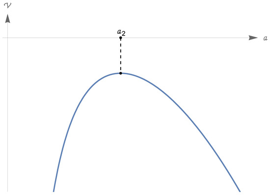
Let be a maximal zero-energy solution; this can be analyzed using the general method of Section 5.4. Due to (188) (and to (144)), the range of the solution is the whole and never vanishes, thus having a constant nonzero sign. It turns out that the domain of the solution is a time interval unbounded from above if , and unbounded from below if . After a time translation , this interval can be reduced to the form if , and to the form if ; as usual for the standard model, hereafter, we consider the case .
In this case, for t ranging in , increases monotonically from 0 to according to the following law (from (148)):
(with ; this function vanishes for , so the above integral is nonsingular). Equation (189) and the first relation (184) imply
of course, the vanishing of the scale factor in this limit indicates a Big Bang. For , an exponential behavior can be predicted for since (by (147) and the second relation (184)) .
The concavity features of the function are inferred from Equation (152) , from Equation (186) about , and from the previous description of this solution. Clearly, there is a unique
and for , for . These facts imply
so, is an inflexion point. Needless to say, the present time is uniquely determined by the condition (recall the discussion in the final part of Section 6.1). According to Equation (189),
Figure 2 describes qualitatively the behavior of the scale factor . Making reference to the formal notions of singular or nonsingular behavior in Section 3.2 and Section 3.15 (here, applied to the time domain ), we can say that the spacetime under consideration is past timelike and lightlike singular since it violates conditions (65) and (66). By contrast, this spacetime is future timelike and lightlike nonsingular since it fulfills (67) and (68).
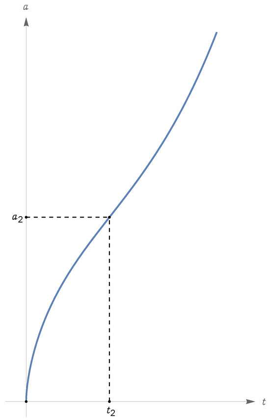
Let us recall that the comparison between observational data [72,73] and the standard model suggests specific values for the normalized energy densities at the present time, which, in our language, correspond to the following prescriptions:
these reference values will be taken into account in the sequel.
To fix the ideas, let us assume exactly the above numerical values for , and set , (so that (181) holds exactly). Using these values and solving Equation (185) for (i.e., numerically), we obtain
From these values and from Equation (193), we obtain (computing numerically the corresponding integrals)
Using Equation (59) involving the present-time Hubble parameter, we infer that the cosmic times () have the values
of course, represents the present age of the universe.
We could continue our analysis and point out other facts, corresponding to known features of the standard model. Here, we will just remark that Equation (188) still holds for and not too large, while this equation fails for and sufficiently large (i.e., for large enough); in the latter case, the behavior of the scale factor is qualitatively different from that described here, as pointed out, e.g., in [75].
6.3. Introducing the Analysis of Cases with
Maintaining all the assumptions of Section 6.1, we now pass from the case (the standard model of cosmology) to cases with ; these will be treated assuming frequently that is small. The deviation of these cases from the standard model is controlled by the term in Equation (168) for .
In the sequel, most of our attention is devoted to the case
- (i)
- (phantom scalar field), (typically small), (i.e., );
this will be analyzed in detail in Section 6.5, Section 6.6 and Section 6.7. In comparison with the standard model of cosmology with , case (i) exhibits an important qualitative difference: instead of the Big Bang of the standard model, there is a Big Bounce, with a minimum value (possibly very small but nonvanishing) for the scale factor.
For , in case (i), the scale factor presents an exponential growth similar to that of the standard model with ; the same exponential growth appears for , i.e., very far in the past before the Big Bounce. As we shall see, specifying values close to those in (194) for and and an extremely small value for , we obtain a Big Bounce model with a minimum of physical plausibility; this could perhaps be considered a non-absurd alternative to the standard Big Bang cosmology.
We will subsequently address the case
- (ii)
- (phantom scalar field), (typically small), (i.e., );
this will be sketched in Section 6.8. If (i.e., k) is below a threshold value, the behavior of the model is similar to that of case (i), with a Big Bounce and exponential growth of the scale factor for . If is above the threshold, the scale factor oscillates periodically (with a positive minimum) or, alternatively, it exhibits a Big Bounce with a (typically large) minimum value and exponential growth for (different behaviors occur if has exactly the threshold value; see again Section 6.8). The physical plausibility of the model when is above (or equal to) the threshold is dubious; to say the least, further investigations on this issue would be necessary.
Finally, in this paper, we will not discuss the case
- (iii)
- (canonical scalar field), ;
this presents a Big Bang19 and can be considered, at least for small , as a perturbation of the standard model of cosmology.
6.4. Preparing the Analysis of the Phantom Case with
From here to the end of the present Section 6, we assume the scalar field is a phantom:
We consider solutions of the model with nonvanishing; for future convenience, we represent this quantity as
We confirm the general conditions (165), (176), and (177), thus requiring that
(note that is just the expression for following from (199); the sign of is unspecified for the moment; of course, all comments after Equation (177) apply here). The potential of Equation (168) is given in the present case by
Needless to say,
6.5. The Phantom Case with (Small) and : Analysis of the Potential and the Associated Function
Throughout the present Section 6.5, we make the assumptions (198)–(200) and also prescribe
(i.e., ). In the sequel, we will often put conditions of smallness on (i.e., on ); the most important of such conditions will be the forthcoming inequality (211).
The potential . In Appendix L (which makes reference to the preceding Appendix I and Appendix J), we prove the following statements (a)–(d) about :
- (a)
- There is a unique point such thatin addition,and
- (b)
- Letthen, and . Moreover,(Note that the upper bound on in (209) implies the rougher bound ).
- (c)
- Let us consider the derivativeand assumeThen, there are just two points such thatmoreoverso that is a local minimum point, and is a local maximum point for . Also, we have the following (somehow rough) inequalities:
- (d)
Remarks. (i) Figure 3 presents a qualitative plot of the potential under the conditions (198)–(200), (204) and (211). To help visualization, in the figure, and are not so small in comparison with while, for physically plausible choices of the parameters, we have : see the forthcoming Section 6.7.

Figure 3.
Qualitative plot of the function in Equation (201), under the assumptions of Section 6.5.
This plot should be compared with that of the potential in the standard cosmological model (see Section 6.2 and Figure 1).
(ii) Let us consider a -dependent family of models in which
The above requirement of sum one for is the equivalent of the condition of sum one in (200); note that Equation (179) for the present-time normalized energy density of the scalar field gives .
For such a family of models, the quantities are functions of , and it makes sense to discuss their behavior in the limit of vanishing . For , we have
In fact, both the lower and the upper bound for in (209) behave like the right-hand side of (218); similarly, the lower and the upper bound for in (216) behave like the right-hand side of (219).
This function is especially interesting since, according to Equations (156) and (87), along any solution of the cosmological model, we have
where h is the dimensionless Hubble parameter (see Equation (70)) and is the total dimensionless density, including the curvature contribution (see Equation (173)). Of course,
Moreover, has the following features (e) (an obvious fact) and (f)–(i) (proved in Appendix M):
- (e)
- For all , we have
- (f)
- Let us consider the derivativeThen, there is a unique point such thatmoreover,Due to these facts and to the asymptotics (222), is the absolute maximum point of andThe last inequality obviously implies so that, by comparison with (224), we also infer
- (g)
- Letthen, and . Moreover,(Note that the upper bound on in (231) implies the rougher bound .)
- (h)
- (i)
- Then,
Remarks. (i) Figure 4 presents a qualitative plot of the function under the conditions (198)–(200), (204), (211), and (234).
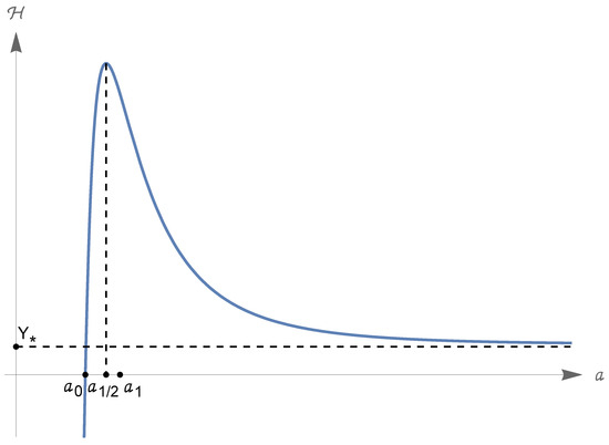
Figure 4.
Qualitative plot of the function in Equation (220), under the assumptions of Section 6.5.
6.6. The Phantom Case with (Small) and : Analysis of the Zero-Energy Solutions and Classicality Condition
Let us consider a zero-energy solution of the reduced system with Lagrangian (141) ( meaning, as usual, an open real interval); we assume this to be maximal, in the sense of Section 4.6, and analyze it according to the general scheme of Section 5.4. Bearing in mind the results of in Section 6.5, we are led to the description reported in the following paragraphs:
Basic features of the solution; Big Bounce. The set coincides in this case with , with as in (205). The motion has range and possesses a unique inversion time , characterized by the condition ; up to a time shift constant, we can assume . Thus,
moreover
(even at , when vanishes). From the quadrature formula (148) with replaced with (or with ), and from Equations (238) and (239), we obtain
Since and , the function diverges like for , so the above integral converges; this remark is related to item (iv) in Section 5.4.
The motion continues until diverges in the far future and in the far past; divergence of occurs for , where . On the other hand, the last integral diverges since for (recall Equation (184)); thus, , and we can say that
(a posteriori, this also ensures that (239) and (240) hold for all ). By construction, the function , solves the Cauchy problem (recall (143)), , . It is evident that the function , solves the same Cauchy problem, so by the standard uniqueness theorem, we have
To summarize, the solution under consideration describes an eternal universe with a Big Bounce at time , when the scale factor attains the nonzero, minimum value ; the history of the scale factor is time-symmetric with respect to the instant of the Big Bounce.
Figure 5 shows a qualitative plot of the scale factor (also taking into account the concavity considerations in the second subsequent paragraph).
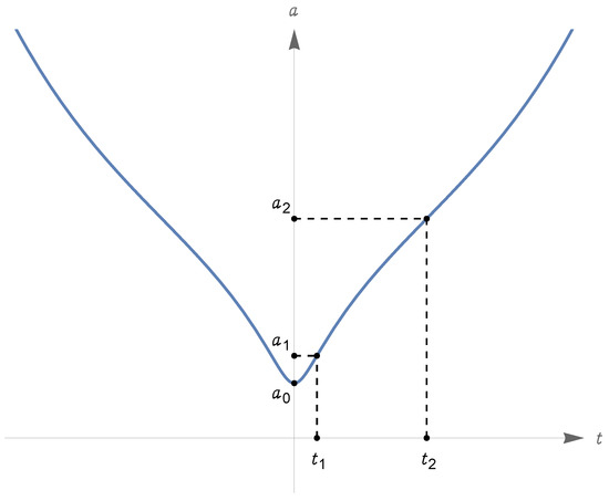
Figure 5.
Qualitative plot of the scale factor , under the assumptions of Section 6.5.
Nonsingular nature of the model. Since the time domain of the model is the whole real axis and the function has a strictly positive minimum, the present spacetime is nonsingular in all senses formalized in Section 3.2 and Section 3.15 (concerning this statement, let us recall Equation (69) and the related comments).
A result frequently used in the sequel. Let . From the features of the function described previously, it appears that there is a unique time
according to Equation (240), this is given by
In the sequel, we will often refer to the above statements.
Concavity features of the solution. Let us reconsider Equation (152) . The sign of is described by Equations (212) and (213) (and by the related Equation (214)), involving two distinguished values such that . For , there is a unique time fulfilling Equation (243), and this is given by Equation (244). Moreover,
Equations (212) and (213) on the sign of and Equations (152), (243) and (245) imply
thus, and are inflection times for the function . One can make similar statements on the behavior of at negative times, noting that (242) implies .
Let us recall that, according to Equation (98), the strong energy condition (SEC) is violated whenever ; in the model that we are analyzing, this happens in the time interval containing the Big Bounce, and in the time intervals , 20. A more detailed analysis of the energy conditions will be presented in the sequel.
The present time. Let us recall the inequality (207) and the considerations after Equations (58) and (99). In the model under discussion, the present time is individuated by the conditions
that automatically imply
In fact, since , and we have the equivalence (161) reviewed in the discussion after Equation (177). The present time is described by Equation (244) with and , i.e.,
In Section 6.7, assuming physically plausible values for the constants of the model, we will find and .
The large t limit: exponential growth of the scale factor. For all , we have ; for , we have and this fact, with Equation (202) about , gives (note that a similar statement was made in Section 6.2). Due to this asymptotic feature, is expected to behave like const.× for . In Appendix N, we rigorously prove that
The integral from 1 to in the above definition of converges, since for (see again Appendix N); let us also recall the expression (249) for .
Needless to say, the relation (250) and the symmetry property also imply
For , let us reconsider the spatial and spacetime line elements (16) and (17) and, referring to the dimensioned time , let us insert the expression for the scale factor corresponding to the right-hand side of Equation (250) into Equation (17); then, the spacetime line element becomes of the de Sitter form (let us recall again [12] (page 125)). In this sense, the present cosmological model with is asymptotically de Sitter for (a feature that also exists in the standard cosmological model with a positive cosmological constant, reviewed in Section 6.2). Due to (251), the present model with is asymptotically de Sitter (in an obvious sense) even for .
The (dimensionless) Hubble parameter . Let us note that Equation (242) implies that h is an odd function of time:
Moreover, due to (239), we have
Let us further discuss the behavior of the function ; it will suffice to see what happens for . With as in Equation (220), we see from Equation (221) that
let us repeat that, while t ranges in this interval, increases monotonically from to . We can combine these remarks with the available information about (see the paragraph starting from Equation (220), and Figure 4); let us recall, in particular, that has a unique maximum point (see Equation (226) and subsequent statements), where (see (229) and (235)), and approaches for (see (222)).
In conclusion, the time behavior of h for is as follows: First of all, there is a unique time such that , and this is given by Equation (244) with . Moreover,
Let us also note that ; in particular, (recalling the relation and Equation (143))
Preliminaries on the densities. Let us consider for the corresponding densities, e.g., in the dimensionless versions ; these are given by Equations (170) and (203), and can be regarded as functions of the scale factor or of the dimensionless time: or . In the sequel, we also refer to the total dimensionless density , including the curvature contribution, which is the sum of all terms (see Equation (173)). Let us remark that the relation implies the following for all :
Time evolution of the total density. Let us recall again Equation (221), ensuring that
for all . The results of the previous paragraph about h yield the following conclusions on the behavior of the function , say for :
(with as in (255)). Let us also note that
Comparison with the Planck density; classicality condition. Let us recall that, in our setting with , the Planck length, time and mass are
From these quantities, we define a Planck density
Let us compare this quantity with the total (dimensioned) density, including the curvature contribution; this is
where is given again by Equation (173), and we have used Equation (169). The comparison can be made by introducing the ratio between the maximum of () and the constant ; due to Equations (259), (261), and (265), we have
where . On the other hand, Equation (264) gives , i.e., by Equation (263),
We note that the parameter Q is dimensionless; using for the values in Equations (59) and (263), we obtain
It is reasonable to prescribe the classicality condition for the cosmological model under analysis, that reads
this ensures, a posteriori, that the classical treatment of gravity given herein is reasonable at any stage of the cosmological model under examination21,22. As we shall see, for small this condition is, essentially, a lower bound on (i.e., on the minimum of the scale factor).
Sign of the phantom energy density, and comparisons among the partial densities. Independent of the previous classicality condition, we now determine the sign of the phantom scalar energy density, and we make comparisons among this density and those associated with radiation, matter, and curvature. Obviously enough, the comparison of these densities gives exactly the same results for any of the available versions (dimensioned, dimensionless, or normalized); hereafter, we refer to the dimensionless versions (), viewing them as functions of the variable on the grounds of Equations (170) and (203)23; let us also remark that for all a, we have and (since we are assuming ).
That said, for any , we have
Again, for any ,
for the proof that exists and is unique, and for a justification of the conditions in (271), see Appendix O. In the same appendix, we prove that
It should be noted that, for small , is very close to : Equations (209) and (273) give the bounds
(with as in Equation (208)). For a family of models as in (217), Equation (273) implies the following for :
(since both the lower and the upper bounds on in (273) behave like the right-hand side of (275)); similarly, we infer from Equation (274) that
To continue, we note that, for any , we have
the existence and uniqueness of , as well as the above conditions , are justified with arguments similar to those employed in connection with Equation (271) and .
Finally, for any , we have
(intending if ).
Let i denote anyone of the above subscripts , . Of course, given the motion , if , there is a unique time such that , and this is given by Equation (244); for any , we have that ⟺ .
On the computation of certain times. Let us consider a time admitting an integral representation of the form (244) , with .
We have already noted that diverges (like ) for ; moreover, we are mainly interested in cases where is an extremely small number. For these reasons, the numerical computation of the integral in (244) is not so trivial. In Appendix Q and Appendix R, the representation (244) is used as a starting point to derive rigorous lower and upper bounds on , which are precise in two different situations; estimation of by means of these bounds is a reliable alternative to the direct numerical computation of the integral in (244). We will return to these issues in Section 6.7.
The analysis in Appendix Q also allows us to consider a family of models as in (217) and discuss the limit for the times , and , which are determined as in (244) with , and (see Equations (212), (226), and (271)). In this limit, it is found that
Time evolution of the scalar field. Equation (136) with and Equation (199), ensure that everywhere on the time domain ,
In particular,
the bounds (209) on , involving as in Equation (208), imply
showing that is very large for small . From (288) and Equations (250) and (251) on the large t behavior of , we also infer that
Again from (288), we see that the function is strictly increasing or decreasing in the two cases ; this agrees with the predictions of item (i) in Section 5.5.
Let us refer to item (ii) in the same section; using Equation (155) therein with and or , and recalling again Equation (199), we conclude that
According to (202), for , we have (while, for , we have ); so, the integral defining converges.
In Appendix S, we derive precise lower and upper bounds on . For a family of models as in (217), these bounds ensure that, in the limit ,
Energy conditions. This subject has been already touched on in a few lines after Equation (246); here, we reconsider it in detail. The weak and strong energy conditions for the general cosmological models considered in this paper are presented in Equations (52) and (53) and reformulated in Equations (93) and (94) in the dimensionless form. In the case under analysis, the space dimension is , and Equations (93) and (94) read as follows:
Again, in the case under analysis, the total dimensionless density and pressure are determined by Equations (170), (203), and (172), which imply
Comparing the above results with the expressions (201), (210), and (225) for the function and for the derivatives we see that25
In the sequel of this paragraph, just for simplicity, we consider the zero curvature case
Due to this assumption, the signs of the quantities in Equation (297) are determined by the signs of , , and , which were studied in Equations (205), (206), (212), (213), (226), and (227) involving the special values . In this way, we find
The equivalent statements in terms of the dimensionless time are obvious; for example, SEC fails for and holds for .
For extending the above results to the case , one should return to Equation (296) and study directly the signs of the quantities appearing therein as functions of a; the problem is dealt with methods very similar to those employed in Appendix L and Appendix M to study the signs of , and .
Comparison with the literature. In Section 5.9, we already mentioned the toy model introduced in [74] (Section II.B), with an FLRW universe of dimension filled only by a canonical or phantom scalar field with zero self-potential. The authors of [74] consider, in particular, the case with a phantom scalar and negative spatial curvature; their analysis indicates (somehow implicitly) that the scale factor exhibits a Big Bounce, while the scalar field tends to finite values very far in the past and the future; we have met the same qualitative behavior in the more realistic model of the present Section 6.6.
6.7. The Phantom Case with (Small), and Specific Values for All the Parameters
Maintaining (198) and (199), we now try to give physically plausible values to the parameters of the model by prescribing
and
The value of the parameter will be fixed later. Let us note that conditions (200) and (204) are satisfied; the same can be said of conditions (211) and (234), if the requirement is intended appropriately. We also remark that Equation (179) for the present-time normalized energy density of the scalar field gives in this case
The above values of , , and are close to the ones ascribed within the standard model of cosmology to the normalized densities of radiation, matter, and dark energy at the present time; the assumption of zero curvature is standard as well (concerning these statements, let us again mention the observational data from [72,73]).
According to Section 6.5, the functions of Equations (201) and (220) can be described referring to some special values of the variable a, such that
in particular, is the minimum of the zero-energy solution analyzed in Section 6.6, to which we systematically refer from now on. We now fix the value of on the grounds of the classicality condition (269); this involves the ratio
with the Planck density (see Equation (264)) and Q as in Equations (267) and (268). However, due to Equations (232) and the smallness of ,
therefore,
where, in the last step, we used the numerical values in Equations (268) and (302) for Q and .
The classicality condition (269) requires the ratio (307) to be very small; we now choose an extremely small value for , which, however, is sufficiently large to fulfill (269). We will adopt the value
implying
From here to the end of the present Section 6.7, we stick to the choices (302) and (308) for , and , confirming that all conditions (200) (204) and (211) (234) are fulfilled; whenever necessary, we use the value (59) for .
In the sequel, we report many distinguished values of the scale factor and the corresponding times (or ), all of them computed on the grounds of the above choices for the basic parameters of this model; the penultimate paragraph of the present section gives some information about these calculations. In the rest of the section, we discuss the sign of the phantom energy density, and we make comparisons among this quantity and the densities of radiation and matter, at any time in the history of this model; moreover, we consider the present epoch.
The values of and the corresponding times. Hereafter, we report the values of the following quantities for : , the dimensionless time such that and its equivalent in terms of cosmic time. Here are the values:
Let us recall that the function is even and, for , increases from the minimum value to . The concavity features of this function are described by Equation (246), indicating that and are inflection points. The time is the maximum point of the Hubble parameter (see Equation (257)) and (we repeat it) of the total density over the interval .
The present time. The present time , individuated by the conditions and , is determined by Equation (249). It is found that and its cosmic time equivalent have the values
is the cosmic time elapsed from the Big Bounce to the present epoch; it is quantitatively indistinguishable from the age of the universe (time elapsed from the Big Bang to now) in the standard model of cosmology (see Section 6.2, in particular, Equation (197))26.
Sign of the phantom energy density, and comparisons among the partial densities. These issues are related to some distinguished values of the scale factor (), described by Equations (270)–(279) and (282)27; the values of are attained at certain times , which have cosmic time correspondents . These special values, arranged in increasing order, are as follows:
Let us consider the evolution of the cosmological model for , recalling that the behavior for is specular due to ; using the inequalities (270), (271), (277)–(279) and (282), we obtain the following description:
- 0.
- . We repeat that and .
- 1.
- , i.e., : a field dominated era, with and ;we repeat that , and .
- 2.
- , i.e., : a radiation dominated era, with .We repeat that and ; according to 0., changes sign shortly after the beginning of this era.
- 3.
- , i.e., : a matter dominated era, with and ; we repeat that and .
- 4.
- , i.e., : a field dominated era, with and . This era contains the present time with and .
For a more detailed description, see Appendix T.
Comparison with the standard model. As stressed after Equation (303), the present-time values for the normalized densities of radiation, matter, and energy of the scalar field in the model of the current Section 6.7 coincide with corresponding values for radiation, matter, and dark energy in the standard cosmological model with curvature ; for the parameter , determining the discrepancy from the standard model, we assumed an extremely small value. The aim of these choices was to produce a model very close to the standard cosmological model at all times subsequent to the Big Bounce, except for an extremely short epoch immediately after the Big Bounce.
The results in the previous paragraphs confirm this expectation: the agreement between the two models has already been exemplified in the discussion on the age of the universe (see Equation (311) and related comments), and many other examples could be extracted from the previous analysis. To give just another example, let us consider the values of the scale factor and of the cosmic time yielding the equality of radiation and matter densities, which are and with our notations; the values of these quantities in Equation (312) agree with the corresponding values in the standard model.
In general, epochs 2, 3, and 4 of the previous paragraph juxtapose (both qualitatively and quantitatively) with the radiation-dominated era, the matter-dominated era, and the dark energy-dominated era in the standard cosmological model. Concerning epoch 4, let us repeat that the present model is asymptotically de Sitter for , like the standard one for (recall the comments after Equations (250) and (251)).
On the first era after the Big Bounce, dominated by the scalar field. This is epoch 1 of the penultimate paragraph, corresponding to the extremely short time interval ; of course, here, the model is significantly different from the standard one. It should be mentioned that epoch 1 is not inflationary, if one defines inflation in terms of an explosive growth of the scale factor: on the contrary, the initial value and the final value of the scale factor are essentially equal (see the first line in Equation (312)).
On the computation of the previous values of and . All computations related to (310)–(312) were performed with more significant digits than those reported here28.
The values of for and the value of were estimated referring to the bounds (209), (216), (231), and (274) and the asymptotic expressions (218), (219), (236), and (276). Due to the extremely small value of , in each one of these cases the numerical values of the lower bound, of the upper bound, and of the asymptotic expression neglecting the reminders , are practically indistinguishable.
By definition, is the second positive solution of the equation (or of the equivalent algebraic equation , where is the polynomial in Equation (A123) of Appendix L); the value of was estimated by solving numerically this equation. The value of was estimated by solving numerically the algebraic equation in (277).
For all choices of i in (310)–(312) we have , as in Equation (244) (note that the present time corresponds to ). Again, for all such choices of i (except , giving immediately ), the time was estimated by direct numerical computation of the integral in (244). To test the reliability of these calculations, we computed the lower bounds, upper bounds, and the asymptotic values for provided by Appendix Q for (see, in particular, the paragraph containing Equation (A200) and the subsequent one). For the same purpose, we computed the lower and upper bounds for provided by Appendix R for (see, in particular, the paragraph containing Equation (A215) and the subsequent one). In all cases, the lower and upper bounds on are indistinguishable from the value provided by direct numerical computation of the previous integral. For , these values are also indistinguishable from those provided by the asymptotic expressions (285)–(287) neglecting the reminders .
Other topics. Of course, all statements in the last two paragraphs of Section 6.6 about the field history and the energy conditions apply to the present framework.
6.8. The Phantom Case with (Small) and : Sketching the Basic Results
(i.e., ). We also put three smallness conditions on ; the first one is Equation (211), the other two are
The potential . Again, this is given by Equation (201) and behaves as in Equation (202) for and . The following facts about are proved in Appendix U.
- ()
- There are just two points as in Equation (212), reproduced here:Moreover, we have again the inequalities (213)so that is a local minimum point, and is a local maximum point for . Also, we have the (rough) inequalities
- ()
- ()
- We have
- ()
- Letthen,The sign of is determined by a comparison between and , and it determines the sign of on as in the forthcoming items () () ().
- ()
- We have the equivalence
- ()
- We have the equivalenceIn the case (324), there is a unique point such that(i.e., has just two zeroes in ). We have again the inequality (322) . Moreover,(see Figure 6).
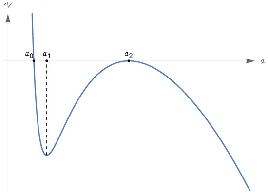 Figure 6. Qualitative plot of the potential in Equation (201), under the general conditions of Section 6.8 and the assumption (324) on the curvature.
 - ()
- We have the equivalence
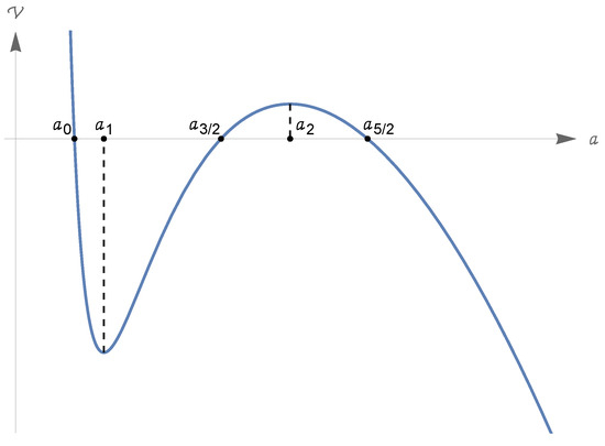 Figure 7. Qualitative plot of the potential in Equation (201), under the general conditions of Section 6.8 and the assumption (327) on the curvature.
 - ()
- In any one of the cases ()–(), we have again the inequality (207) .
- ()
- Letthen, and . Moreover, in any one of the cases ()–(), we have
Behavior of the scale factor. Let us refer to the cases ()–() in the previous paragraph, which correspond, respectively, to the assumptions (320), (324) and (327). Recalling the definitions (146) of , we have the following:
- Under the assumption (320), we have and . The behavior of a (maximal) zero-energy solution is similar to that described in the previous Section 6.6. So, is defined on the whole real axis with image . There is a Big Bounce at a time that we take conventionally to be , with ; moreover, and (exponentially) for .
- Under the assumption (324), we have and , with and ; there are three types of zero-energy solutions, described hereafter.First type: There is a Big Bounce at , and is approached in the past and the future. We can assume the Big Bounce to occur at time , i.e., ; then, for all t. The function increases from to for and decreases from to for . The value is attained at times (see item (vi) in Section 5.4). In conclusion, has domain , range and . See Figure 8, where we also indicated the time such that ; recalling item (viii) in Section 5.4, we see that is an inflection point for the scale factor since and has different signs on the left and on the right of .
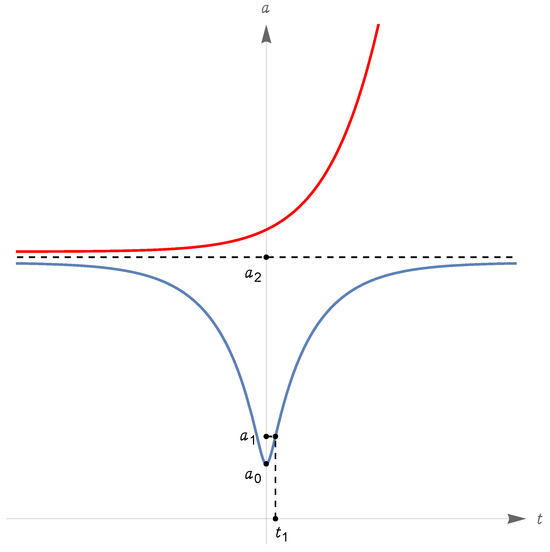 Figure 8. Solutions of the first type (in blue) and of the second type (in red), under the general conditions of Section 6.8 and the assumption (324) on the curvature. The same assumptions yield a third type of solution, namely constant for all real t.Second type: has domain and range ; for all real t, or for all real t. If , we have for and for ; if , the values of the limits for are interchanged (the reason why the time required to reach is infinite is explained again by item (vi) in Section 5.4; the discussion of the time required for to diverge is related to item (vii) in the same section). In Figure 8, we illustrate the case .Third type: This corresponds to the equilibrium solution for all (see item (v) in Section 5.4).
 - Under the assumption (327), we have and , with , and ; there are two types of zero-energy solutions, described hereafter.First type: The function has domain and range ; it oscillates periodically with period(see items (ii)–(iv) in Section 5.4; the above convergent integral gives the time required for the scale factor to pass from to , that equals the time to return to ). This type of motion is represented in Figure 9 (note that the function has inflection points at the infinitely many times t such that ; these times are not indicated in the figure).
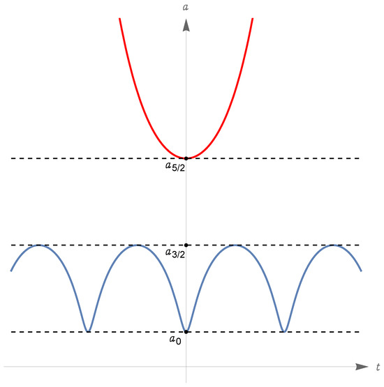 Figure 9. Solutions of the first type (in blue) and of the second type (in red), under the general conditions of Section 6.8 and the assumption (327) on the curvature.Second type: The function has domain and range . There is a Big Bounce at the time when equals , which we can assume to be ; we have for all real t, is strictly increasing (resp., decreasing) on (resp., on ), and (exponentially) for . See Figure 9 again.
 - In all the cases considered above, we have a cosmology with the time domain , in which the scale factor admits a strictly positive infimum. This is nonsingular in all senses considered in Section 3.2 and Section 3.15 (let us recall again Equation (69) and the related comments).
- Since the very beginning of the present study on cosmological models with matter, radiation, and a scalar field with constant self-potential, we have focused on the zero-energy solutions of the reduced system fulfilling at some time the condition , which is indeed equivalent to : see the discussion after Equation (177). Such a condition can either hold or fail for the solutions described above. For example, in the case (327), the requirement that at some time is fulfilled by the zero-energy solutions of the first type if and only if , and the zero-energy solutions of the second type if and only if .
7. Polar and Cartesian Coordinates for Phantom Cosmologies with a Periodic Field Potential
In the present Section 7 (and in the subsequent Section 8) we consider a phantom scalar field, so that
7.1. Polar Coordinates (Under Periodicity Assumptions for the Field Potential)
Let us consider the Lagrangian L of Equations (121) and (122) with , and pass from the coordinates and to the new coordinates and , defined by
The Lagrangian as a function of the new coordinates, again indicated with L, is
(the ’s are as in Section 4.1 and Section 4.2). Let us note that is the kinetic energy of a particle (of unit mass) in a Euclidean plane, equipped with polar coordinates; the other summands in the Lagrangian (336) can be interpreted as potential energy terms, depending on r and .
As a matter of fact, for a genuine interpretation of as polar coordinates it is required that29
due to the relation between and in (335), (338) holds if and only if
This makes some difference with respect to the general setting employed up to now, where is the dimensionless form of the scalar field , and these two objects are connected by the relation (73) . Indeed, to make (339) compatible with (73), we must slightly modify the general setting for the scalar field in Section 2.3, Section 3.1, Section 3.2, Section 3.3, Section 3.4 and Section 3.5, and assume30:
Of course, to be consistent with the viewpoint (339) and (340), we must assume that the dimensioned field potential and its dimensionless version are (smooth) functions
still connected through the relation (74) . In the same vein, Equation (337) defines a function
It should be noted that a function as in Equation (341) can be identified with a periodic function of period ; similarly, the functions in Equations (341) and (342) can be identified with periodic functions of periods and , respectively.
In the present Section 7 and in the subsequent Section 8, we will stick to the setting (338)–(342). The transformation defined by Equation (335) is a smooth diffeomorphism between and . The Lagrangian (336) is a function of the variables , and depends on the smooth functions , defined by Equation (337).
7.2. Cartesian Coordinates
Maintaining the setup of the previous Section 7.1, we can pass from the polar coordinates to the Cartesian coordinates
Obviously enough, the above transformation is a smooth diffeomorphism between and , whose inverse map can be described via the following equations:
8. An Explicitly Solvable Phantom Model with Dust and a Trigonometric Field Potential
8.1. Some Introductory Considerations
In Section 5 and Section 6, we have shown that the evolution equations of the cosmologies considered in this paper can be reduced to quadratures when the potential of the scalar field is constant (or, equivalently, in the presence of a cosmological constant). Of course, one would like to individuate solvable cosmological models with a nonconstant field potential.
In the current Section 8, we will present a phantom model with dust and a trigonometric field potential, which is explicitly solvable. A nice feature of this model is that the evolution equations, when written in Cartesian coordinates following Section 7, describe two uncoupled one-dimensional systems, each one interpretable as a harmonic repulsor, a harmonic oscillator, or a free particle. In the case of two harmonic oscillators, the trajectories of the cosmological model in the plane are the Lissajous curves [63,64], mainly popular for non-cosmological reasons.
In Section 8.2, we give a detailed presentation of the model, including the explicit form of the potential for the phantom scalar (see Equations (350) and (351)); admittedly, the main motivation for this choice of the potential is to produce a system with the beautiful mathematical features outlined before. In the final paragraph of the same section, we make comparisons with the previous literature. In the subsequent Section 8.3, Section 8.4, Section 8.5, Section 8.6, Section 8.7, Section 8.8, Section 8.9, Section 8.10 and Section 8.11, we analyze the solutions of the model and their physical meaning, in a number of qualitatively different cases.
8.2. Introducing the Solvable Model
Let us stick to the general framework of Section 7. The setting introduced therein is specialized in the following way:
- There is only one perfect fluid of the dust type, i.e., with zero pressure. Thus,(to determine the expression of , we used Equation (114) with ); in the sequel we refer to this fluid with the generic denomination of “matter”. We assume the spatial curvature vanishes, so
- The function of Equation (337), giving the potential of the scalar field in terms of the coordinate , is assumed to have the form
Due to Equations (349) and (350), the Lagrangian (336) reads
passing to the Cartesian coordinates (343), we have
The corresponding energy function reads
and the Lagrange equations are
Equation (355) concerns two uncoupled systems. The x-system can be described as a harmonic repulsor if , a harmonic oscillator if , and a free particle if ; a similar description, depending on the sign of , can be given for the y-system.
In the sequel, we frequently use the vector variable
so that the radius coincides with usual norm ; we will generically indicate with boldface symbols the elements of and set .
Let us recall that we are interested in the solutions of the Lagrange equations taking values in and fulfilling the energy constraint (see Section 4.4). For any such curve, the instantaneous distance between the point and the origin gives the radius and, consequently, the scale factor via Equation (335). The angle and, consequently, the field can be obtained from Equations (344) and (335), but the related calculations will not be reproduced in the forthcoming examples.
Let us return to the constraint . Due to Equation (354), this reads
the right-hand side of (357) is automatically constant along any solution of the Lagrange equations (355), and we can use (357) to determine for any given solution. However, we must keep in mind our requirement . If and (two harmonic oscillators), the right-hand side of (357) is positive along any solution of the Lagrange equations with values in . The positivity of the right-hand side is not granted for different choices of the signs of ; in these cases, the positivity requirement selects a distinguished subclass of solutions of (355).
In the forthcoming sections, we will present several examples of the above general scheme, corresponding to specific choices for and . None of the cases treated in the sequel will include an explicit analysis of the energy conditions; however, in most cases, there are violations of such conditions of some of the types in Equations (97) and (98).31
Connections with the previous literature. The solvable model with a phantom scalar and dust proposed in the present Section 8 was considered by Capozziello, Piedipalumbo, Rubano, and Scudellaro [25] in the special case (and )32. Our present model with arbitrary and produces a larger variety of behaviors in the solutions of the model, allowing, e.g., for the Lissajous cosmologies mentioned before. Since the choice has already been treated, we will not reconsider it in the sequel (and we will not even discuss the very similar case ).
A system decoupling in two harmonic repulsors/oscillators/free particles also arises from certain FLRW cosmological models with a canonical scalar field and (possibly) dust, where the self-interaction potential for the scalar field has an exponential form; these were analyzed by de Ritis, Marmo, Platania, Rubano, Scudellaro and Stornaiolo [26] (without dust); Dereli and Tucker [77] (again, with no dust); Rubano and Scudellaro [28]; Piedipalumbo, Scudellaro, Esposito and Rubano [27], Fré; and Sagnotti and Sorin [30] (without dust: see Section 3.2.1 in this reference), as well as in subsequent works by some of us: the Ph.D. thesis [31] and the paper [32] with D. Fermi. In all these works, the separation coordinates yielding the above decoupling have a different geometrical meaning in comparison with the coordinates in our Equation (355): here, we use two orthonormal Cartesian coordinates in a Euclidean plane, while the separation coordinates in the cited works must be interpreted as orthonormal coordinates in flat, two-dimensional Minkowski space33,34.
For completeness, let us mention that some (not explicitly solvable) models with two coupled repulsors or oscillators have been considered by Castagnino, Giacomini, and Lara [79]; Carroll, Hoffman, and Trodden [20]; and Faraoni [80] as exact or approximate descriptions for FLRW cosmologies with canonical or phantom scalar fields. While repeating that the x and y subsystems in our Equation (355) are uncoupled, let us confirm that they describe exactly an FLRW cosmology with a phantom scalar (and dust).
To continue, we refer to the paper by Chervon and Panina [40] about solutions of FLRW cosmological models with a phantom scalar (and no type of matter); here, the authors present exact solutions for a list of self-interaction potentials, individuated by the superpotential method (see the Introduction). The list in [40] contains potentials of exponential and of other types but does not include the trigonometric potential analyzed in the present Section 8.
A trigonometric self-interaction potential was considered by Ivanov [38] within an FLRW cosmological model with a canonical scalar field (and no matter content); an exact solution of this model was derived in the cited work (and reconsidered in the book [37] via the generating function method; see again the Introduction).
8.3. The Case ()
If and are both positive we can represent them as indicated in the title, with ; in this case, Equation (355) describes two harmonic repulsors.
In the forthcoming Section 8.4, we will treat the case ; this gives once more a model with a constant potential for the phantom field (i.e., with a cosmological constant), which deserves consideration since it admits a particularly nice geometric interpretation. In the subsequent Section 8.5, we will treat the general case with and considered arbitrary, which gives a nonconstant field potential whenever .
8.4. Cosmologies with
Let
This prescription corresponds to a constant and positive field potential since Equations (350), (351), and (358) give
The case with a constant field potential was discussed in general in Section 5, for arbitrary choices of the matter fluids and of the curvature; according to Equations (130)–(132) at the beginning of the cited section, the present form (359) of V corresponds to a positive cosmological constant
Of course, we could solve the cosmological model under analysis specializing the framework of Section 5 to the present subcase with dust and zero curvature; however, the same conclusions can be obtained in the present setting in a simpler and more geometrical way. For this purpose, we write the evolution equations (355) and the expression (357) for the density parameter with (), using the vector variable and the standard norm of . In this way, we obtain
(Let us repeat that coincides with the usual radius r.) As recalled in Appendix V, a function is a maximal solution of Equation (361) if and only if one of the following cases (i)–(iii) occurs:
- (i)
- We have
- (ii)
- We have
- (iii)
- Up to a time translation const., we havewhere( is the standard inner product of ; the previous conditions on indicate that this pair is an orthonormal basis of ).
In the sequel, we will not consider the trivial cases (i) and (ii) and we will fix the attention on case (iii), which we will discuss with the nondegeneracy assumption
Assuming (367), let us write Equation (365) as
for all we have
and we recognize that the point describes a branch of a hyperbola (see Figure 10). Let us remark that for all .
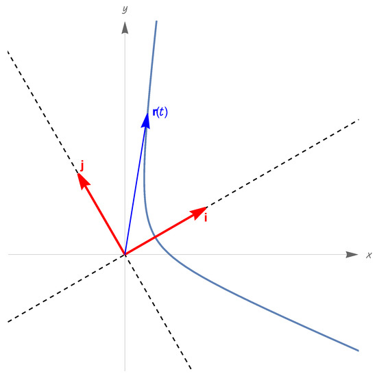
Figure 10.
The branch of hyperbola described by , in the framework of Section 8.4.
From here, it is evident that is a point of absolute minimum for the function , with
it is also evident that and that the function is strictly decreasing on , strictly increasing on (see Figure 11). Finally,

Figure 11.
Graph of the radius , in the framework of Section 8.4.
The above features of the radius function are easily rephrased in terms of the scale factor (recall Equation (335)). Thus, the function has an absolute minimum at , with ; this function decreases strictly on , increases strictly on , and grows exponentially for .
To summarize, the present cosmological model presents a Big Bounce at ; note that the minimum value (or ) can be made arbitrarily small by choosing a sufficiently small A. Needless to say, the strict positivity of the minimum ensures this cosmological model to be nonsingular, in all senses considered in Section 3.2 and Section 3.15 (let us recall again Equation (69) and the related comments).
8.5. Cosmologies with and Arbitrary
We now discuss the general case
(this will also give an alternative treatment of the special case , already discussed in the previous section by different means). Equation (355) reads
a function is a maximal solution of these equations if and only if
where
For simplicity, from now on, we just consider the nondegenerate case
Let us investigate conditions under which or vanish. For any , we readily find the following equivalences:
Clearly, the function has a zero if and only if the conditions on the parameters indicated above hold, and the above zeroes of and coincide; the last condition means equality of the times (). Thus,
To continue, let us note that Equation (357) with and Equation (377) give
we want , so from now on we also assume
Let us proceed to the analysis of the (never vanishing) radius . Equation (377) gives
from here, we infer that
The function defined above has derivative , and for . Thus, is strictly increasing with range ; therefore, there is a unique
and for , for .
Since for all real t, we conclude the following: the radius function admits as a point of absolute minimum, is strictly decreasing on and strictly increasing on (we know that for all t, this holds, in particular, for the minimum value ). Finally, let us remark that Equation (387) implies
where are defined as follows: If , then , , and ; if , then , , and ; if , then, , and .
The above results on the radius function imply similar statements on the scale factor given by (335). Thus, the function has a (strictly positive) absolute minimum at , decreases strictly before , increases strictly after , and diverges exponentially for . Again, we have a model with a Big Bounce; this is nonsingular in all senses considered in Section 3.2 and Section 3.15, due to Equation (69) and related comments.
In Figure 12 and Figure 13, we report, respectively, the range of the curve and the graph of the radius for a special choice of the parameters, compatible with (383) and (386).
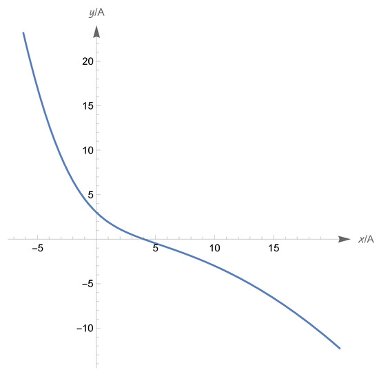
Figure 12.
With reference to Section 8.5, let , , , , , with arbitrary . The curve in blue is the range of as a function of the variable , for .

Figure 13.
With reference to Section 8.5, let the parameters be fixed as in Figure 12. The curve in blue is the graph of as a function of the variable , for .
8.6. The Case (): Lissajous Cosmologies
We now address the case where and are both negative and represent them as
Then, Equation (355) reads
and describes two uncoupled harmonic oscillators with pulsations . A function is a maximal solution of (392) if and only if, up to a time translation const., it can be expressed as follows:
where
The curves in corresponding to the solutions of (392) are the familiar Lissajous curves; as is well known, these curves exhibit a variety of different qualitative behaviors, depending mainly on the ratio and on the phase (see the already cited references [63,64]). In the sequel, for particular values of , we will represent the solutions of (392) in specific forms, different from (393), although equivalent to it, which will be more useful to describe the cases in consideration.
Let us recall that, in view of our cosmological model, we are interested in curves (or portions of such curves) with . Let us also remark that Equation (357) with and Equation (393) imply the following expression for the density parameter:
In the forthcoming Section 8.7 and Section 8.8, we will discuss as examples the cases and ; in Section 8.9, we will present some general facts about Lissajous cosmologies (and we will also mention another example).
8.7. Lissajous Cosmologies with
Let us consider the case
This corresponds to a constant and negative field potential since Equations (350), (351), (391), and (396) give
Let us repeat that the case with a constant field potential was discussed in general in Section 5, for arbitrary choices of the matter fluids and of the curvature; according to Equations (130)–(132) at the beginning of the cited section, the present form (397) of V corresponds to a negative cosmological constant
Apart from the negative sign of the potential, the situation we are considering here is conceptually similar to that discussed in Section 8.4 from which we reproduce the following comment: we could solve the cosmological model under analysis by specializing the framework of Section 5 to the present subcase with dust and zero curvature, but the same conclusions can be obtained in a simpler and more geometrical way from the present setting. For this purpose, we write the evolution equations (355) and the energy constraint (357) with for , using the vector variable (and the standard norm of ); in this way, the cited equations become
As recalled in Appendix W, a function is a maximal solution of Equation (399) if and only if, up to a time translation const., it has the form
involving the parameters
(again, denotes the standard inner product of ; the above conditions on indicate that this pair is an orthonormal basis of ). It is evident that the function in Equation (401) is periodic of period .
Let us rephrase Equation (401) as
It is evident that
so we have an ellipse: the minor semiaxis has direction and length A, while the major semiaxis has direction and length B (see Figure 14). Of course, for all .
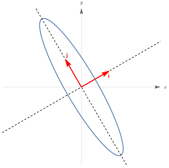
Figure 14.
The ellipse described by , in the framework of Section 8.7.
The radius is given by
this is a periodic function of time, with period (see Figure 15). Clearly, we have
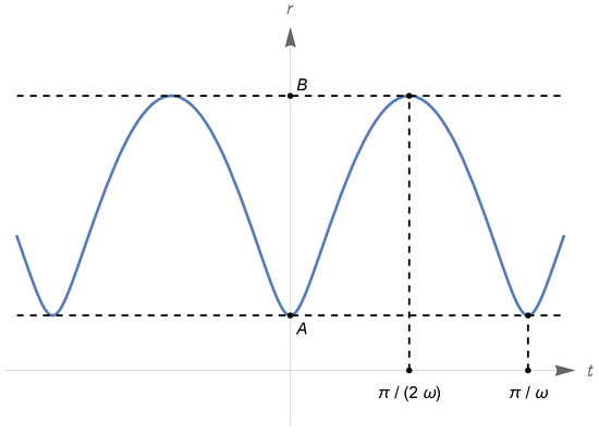
Figure 15.
Graph of the radius , in the framework of Section 8.7.
Let us recall that the scale factor is related to through Equation (335); we have again a periodic function of period , with
Of course, this cosmological model is nonsingular in all senses considered in Section 3.2 and Section 3.15, due to Equation (69) and related comments.
Choosing appropriately A (resp., B), we can make the minimum of arbitrarily small (resp., the maximum of arbitrarily large); moreover, the period can be made arbitrarily long by choosing a sufficiently small .
The special case . In this case, the ellipse described by Equation (405) becomes a circumference of radius A; thus, const. and const. . Consequently, the spacetime line element in Equation (17) becomes ; let us recall that we are assuming zero spatial curvature, so is the line element of the flat d-dimensional Euclidean space. Due to these facts, spacetime is the flat, -dimensional Minkowski space. According to the Einstein equations, the total stress–energy tensor must be zero in this case; to obtain this result, contributions to stress–energy tensor from dust and the phantom scalar must counterbalance.
8.8. Lissajous Cosmologies with
Let us consider the case
The maximal solutions of (392) can be represented as in Equation (393) with the above values for the pulsations. We will consider only nondegenerate cases with and we will employ the reparametrizations , ; thus,
where
For future use, we also introduce the parameter
whose relevance will appear in the sequel (with the above limitation on R). The function in Equation (412) is clearly periodic, of period . As is well known, the shape of the Lissajous curve described by is very sensitive to the phase . Figure 16 describes the familiar curves corresponding to the choices (); by a reflection we also obtain the curves with (), since . For any , Equation (395) for the mass density parameter gives
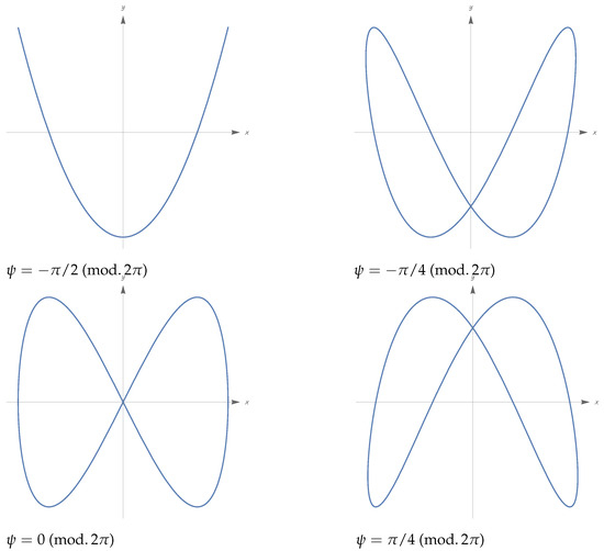
Figure 16.
Lissajous curves with and several choices of the phase .
Hereafter, we will consider the cases () as examples, which will be treated in detail.
The case (). We have
(with , as assumed before); the functions never vanish simultaneously, so
To continue, let us remark that ; so,
Thus, the Lissajous curve we are considering is a parabolic segment with the y axis as a symmetry axis, vertex and endpoints , where
(see Figure 17 and Figure 19). Let us allow t to range in the time interval , whose length corresponds to one period of the function ; then the point describes twice the parabolic segment, from to and back to . In particular,
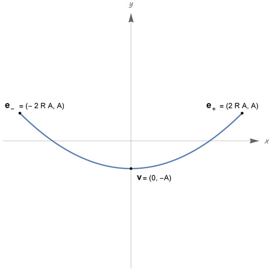
Figure 17.
Lissajous cosmology with and (), (see Section 8.8). The parabolic segment in blue is the range of the map .
Of course, a similar description of the behavior of can be given for t ranging in any time interval ().
Due to (416), the (never vanishing) radius is given by
this is a periodic function of time, of period , and . It is readily found that, for all ,
The sign of is readily studied, and one concludes the following on the behavior of over one period, e.g., on the interval :
Case : behaves as follows on . The times are absolute maximum points, 0 is an absolute minimum point, and
The function is strictly decreasing on and strictly increasing on . From a geometrical viewpoint, the above results indicate that the points of the parabolic segment maximizing the distance from the origin are ; the point minimizing the distance from the origin is . See Figure 17 and Figure 18.
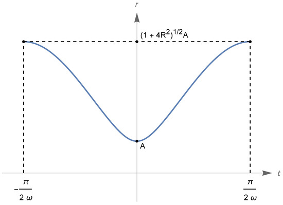
Figure 18.
Lissajous cosmology with and (), (see Section 8.8). Plot of the radius over a period.
Case : Let us consider the times
with as in Equation (414); then,
and the function behaves as follows over one period . The times are absolute maximum points and 0 is a relative maximum point, with , and as in (423). The times are absolute minimum points, with
The function is strictly decreasing on and on , strictly increasing on and on .
From a geometrical viewpoint, the above results indicate that the points of the parabolic segment maximizing the distance from the origin are . The points minimizing the distance from the origin are
(the above explicit expressions for follow from Equations (416) and (424) for , and for the times involved). See Figure 19 and Figure 20. Both for and for , the behavior of the function on any interval () is of course similar to that described above for . One can choose A and R so that the absolute minimum of is arbitrarily small and the absolute maximum of is arbitrarily large. Also, the periods involved can be made arbitrarily large by choosing sufficiently small.
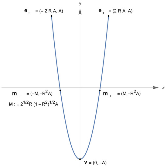
Figure 19.
Lissajous cosmology with and (), (see Section 8.8). The parabolic segment in blue is the range of the map .
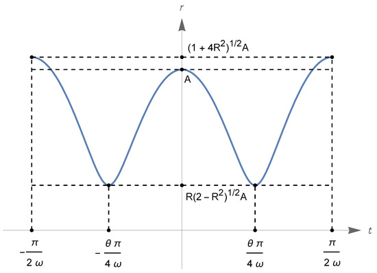
Figure 20.
Lissajous cosmology with and (), (see Section 8.8). Plot of the radius over a period.
Of course, analogous conclusions hold for the scale factor given by (335): this is a periodic function of period , with maxima and minima at the times indicated above for the function . Equation (69) applies once more to the model under examination and ensures that this cosmology is nonsingular in all senses considered in Section 3.2 and Section 3.15.
The case (). Equation (412) gives
(with , as assumed before); the corresponding Lissajous curve is described in Figure 21 and Figure 24. For all , we have
moreover,
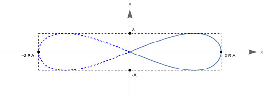
Figure 21.
Lissajous cosmology with and (), (see Section 8.8). The curve in blue is the range of the map for t in the domain of the cosmological model. The dashed curve in blue is the range of the map for .
The existence of zeroes of for is an exceptional feature of the present case (), which also appears for (): on the contrary, for any and for any , the solution described by Equation (412) is such that for all 35.
Keeping in mind (430), we build the present cosmological model restricting the solution to a maximal interval such that for all ; we can take for any . The choice of k is immaterial, and we will set , i.e.,
this will be our time domain from now on.
It is readily found that, for all ,
The sign of is readily studied, and one concludes the following on the behavior of over the interval :
Case : is an absolute maximum point and
The function is strictly increasing on and strictly decreasing on ; see Figure 22. More geometrically, considering the curve (see again Figure 21), we can say that the point of this curve maximizing the distance from the origin is
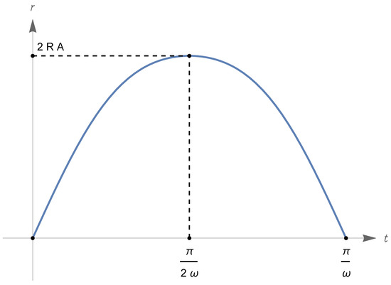
Figure 22.
Lissajous cosmology with and (), (see Section 8.8). Plot of the radius over the domain .
With appropriate choices of A and R, the maximum can be made arbitrarily large.
Case : Let us consider the times
with as in Equation (414). Then,
and the function behaves as follows on . The times are absolute maximum points and is a relative minimum point, with as in (435) and
The function is strictly increasing on and on , , strictly decreasing on and on ; see Figure 23.
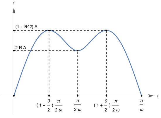
Figure 23.
Lissajous cosmology with and (), (see Section 8.8). Plot of the radius over the domain .
More geometrically, considering the curve (see again Figure 24), we can say that the points of this curve maximizing the distance from the origin are
the latter distance has a relative minimum point at as in (436).
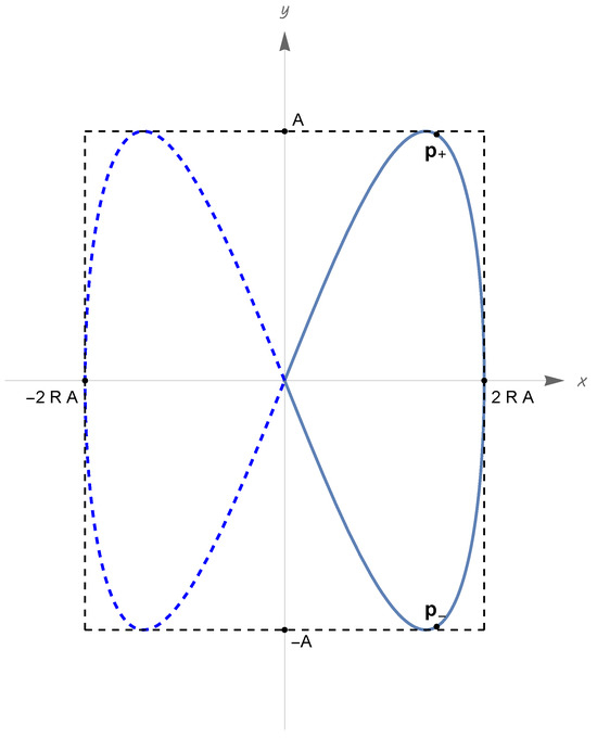
Figure 24.
Lissajous cosmology with and (), (see Section 8.8). The curve in blue is the range of the map for t in the domain of the cosmological model; are the points maximizing the distance from the origin (see Equation (440)). The dashed curve in blue is the range of the map for .
With appropriate choices of A and R, the maximum can be made arbitrarily large, and the relative minimum arbitrarily small. Finally, the time interval can be made arbitrarily long by choosing a sufficiently small .
Our conclusions about the radius have obvious analogs for the scale factor , given by (335). Both for and for , vanishes for ; so, the evolution of this model starts with a Big Bang at , and ends with a Big Crunch at . If , has an absolute maximum point at time ; if , has two absolute maximum points at times , and a relative minimum point at . The occurrence of a Big Bang and a Big Crunch is strictly related to the existence of zeroes of and therefore reflects the exceptional feature of the case () mentioned after Equation (430).
Let us remark that the model under consideration is singular in any one of the senses considered in Section 3.2 and Section 3.15: in fact, any one of conditions (65)–(68) is violated in this case (needless to say, the times appearing in the cited equations are 0 and in the present case).
8.9. On General Lissajous Cosmologies
Let us spend a few words on the general case (391) (), where are chosen arbitrarily in . We know that the maximal solutions of the evolution equations (392) have the form (393), depending on the constants as in (394). Here, we only consider the nondegerate case , so that
Let us also recall that the zero-energy constraint gives the expression (395) for the mass density parameter.
Periodicity conditions for the function . From Equation (441), it follows that the function is periodic if and only if is rational, i.e., if and only if
in this case,
In the same case, we have a periodic cosmological model provided that for all ; whether or not this happens depends on the phase , as illustrated in the next paragraph.
Of course, the cases considered in Section 8.7 and Section 8.8 fit condition (442). As a further example, let
Equation (442) clearly holds with , and Equation (443) ensures the function to be periodic of period . In Figure 25, we illustrate the range of this function for several choices of the phase (assuming for simplicity ); we will return to this example in the final paragraph of the present section.
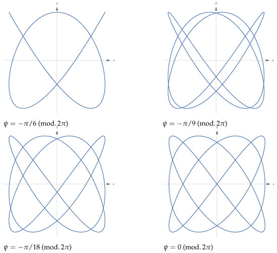
Figure 25.
Lissajous curves with and several choices of the phase .
If is irrational, it can be shown that the range of the (non-periodic) function densely fills a rectangle centered at the origin in the plane [64]: see Figure 26. Again, the function is never vanishing or possesses zeroes, depending on the phase . If never vanishes, the radius (hence, the scale factor in (335)) is always positive but becomes arbitrarily small at suitable times, due to the above-mentioned density result; it should be mentioned that the functions are almost periodic, in the rigorous sense given usually to this expression (see [81], page 1).
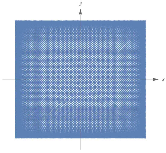
Figure 26.
If is irrational (and ), the range of the map densely fills a rectangle.
When does vanish? We will discuss the problem for arbitrary and , with either rational or irrational; for this purpose, we choose any real representative of the phase , so that
Let us first individuate the times t at which and vanish separately. From Equation (441) (with replaced by ), one easily infers the following, for any :
This implies the following statement about ):
where
We can rephrase the result (448) in terms of the phase , which is represented by ; after noting that (mod. ) equals (mod. ) or (mod. ) for even or odd, respectively, we conclude that
Let us note that, for any choice of , we have (if , it is evident from (441) that ). To continue our discussion on the zeroes of , we must distinguish the cases with rational or irrational.
The case of rational : In this case, which is described by Equation (442), Z is a finite subset of 36. For each phase , the periodicity of (see Equation (443)) implies that there are infinitely many times such that .
The case of irrational : In this case, the subset Z is infinite and dense in ; however, Z is countable, so its Lebesgue measure is zero. For each phase , there is a unique time such that 37.
A final comment: We have just noted that, depending on the rational or irrational nature of , the phases giving rise to zeroes for form a finite or an infinite but countable, zero-measure subset of . In both cases, these phases must be regarded as exceptional.
Nonsingular Lissajous cosmologies. Given , let us consider a phase outside the exceptional set Z of Equation (450) and any two amplitudes . Then, for all , and we have a cosmological model with time domain , in which given by Equation (335) is nonvanishing for all real t.
We claim that this cosmological model is nonsingular, in all senses considered in Section 3.2 and Section 3.15. Indeed, if is rational, the function on is periodic (let us recall again Equation (443)), and this implies periodicity of the functions . Thus, , and this suffices to infer all nonsingularity conditions in the above sections (let us recall once more Equation (69) and the related comments).
If is irrational, the functions , on are not periodic, and (recall the statements on the irrational case after Equation (444)); nevertheless, all nonsingularity conditions (65)–(68) are satisfied, since it can be checked directly that all integrals in the cited equations are divergent38.
Singular Lissajous cosmologies. Given , let us consider a phase in the exceptional set Z of Equation (450), and any two amplitudes . Then, according to the discussion after Equation (450), the function has infinitely many zeroes if is rational and unique zero if is irrational. To establish a cosmological model, we must confine the time variable to a maximal interval not containing zeroes. In the rational case, we will have , where are two consecutive zeroes; in the irrational case, or , where is the unique zero. The scale factor , determined by (335) vanishes for or for . So, in the rational case, the model has a Big Bang at and a Big Crunch at , whereas in the irrational case, there is either a Big Bang or a Big Crunch at .
With reference to the formal notions of singular or nonsingular spacetime of Section 3.2 and Section 3.15, we can state the following:
- In rational case, where , the model is singular in any one of the senses considered in Section 3.2 and Section 3.15: in fact, any one of conditions (65)–(68) is violated (of course the times in the cited equations coincide with and , respectively).
Regarding an example mentioned previously. Let us return to the example (444) , (; needless to say, , as in (441)). Let us repeat that Equation (442) holds with and that, due to (443), the function is periodic of period .
Using Equations (449) and (450), we see that the set of exceptional phases giving rise to zeroes for the function is ; for all the other phases , we have nonsingular, periodic Lissajous cosmologies. We have already mentioned Figure 25, related to this case; the phases considered therein include the exceptional choice ()40.
8.10. The Case
We finally address the case
Equation (355) reads
thus describing a repulsor and an oscillator. A function is a maximal solution of these equations if and only if it can be expressed as follows, up to a time translation const.:
where
In the rest of the present Section 8.10, we direct our attention to the nondegenerate case
Let us investigate conditions under which or vanish. For any , we readily find the following equivalences:
Clearly, the function has a zero if and only , and the zero of indicated in (456) coincides with one of the zeroes of described by (457); the last condition holds if an only if for some . Thus,
From here to the end of the present Section 8.10, we assume
since we are denying the conditions on in (458), we have
To continue, let us note that Equation (357) with , and Equation (453) give
we want , so, from now on, we also assume
Let us proceed to the analysis of the radius ; Equation (453) gives
Of course,
Moreover, if , we can expect an oscillatory behavior of the radius in an interval around the time (with for each , due to (460)); oscillations should be particularly evident if .
Similar statements hold for the scale factor (), related to r via Equation (335); in a few words, in this cosmological model, the scale factor diverges exponentially for and oscillates (but never vanishes) during a time interval centered at . In particular, exists and is strictly positive; so, due to Equation (69) and related comments, the present cosmological model is nonsingular in all senses considered in Section 3.2 and Section 3.15.
The situation under analysis is presented in Figure 27, for a special choice of the parameters; Figure 28 represents the curve for the same values of the parameters.
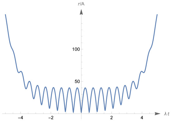
Figure 27.
With reference to Section 8.10, let the parameters be fixed as in Figure 28. The curve in blue is the graph of as a function of the variable , for .
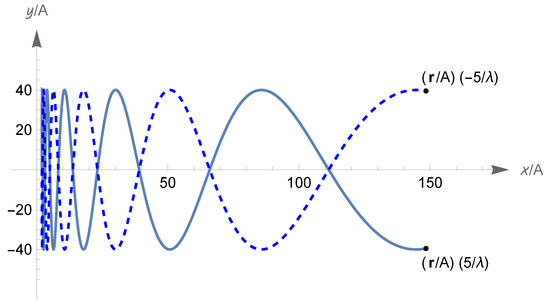
Figure 28.
With reference to Section 8.10, let , and , with arbitrary . The curves in blue are the ranges of the map for (dashed curve) and for (continuous curve); we have indicated the points for .
8.11. Again on the Case ,
As in the previous section, let us make the assumption (451) and (with . Let us recall the evolution equations (452) and the representation (453) and (454) for their (maximal) solutions , depending on three real parameters and .
In the present Section 8.11, we consider some interesting choices for the parameters that were previously ruled out by the conditions (455) and (459).
Case , , . This choice violates condition (455). Equation (453) gives
for all real t, we have and, consequently, . According to Equation (461), the mass density parameter is
The radius function is given by
We have
( means, as usual, a function vanishing in the limit considered above). Thus, the radius oscillates (but never vanishes) for and grows exponentially for ; similar conclusions hold for the scale factor (), which is once more determined by Equation (335). The present cosmological model is nonsingular in all senses considered in Section 3.2 and Section 3.15, since it fulfills all conditions (65)–(68)41.
In Figure 29 and Figure 30, we plot the curve and radius for a specific choice of the parameters involved.

Figure 29.
With reference to Section 8.11, let , and , with arbitrary . The curve in blue is the range of the map for ; we have indicated the point for .
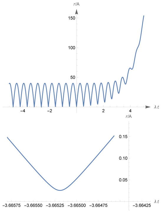
Figure 30.
With reference to Section 8.11, let the parameters be fixed as in Figure 29. The upper picture presents the graph of as a function of the variable , for . The lower picture is a detail of the same graph for in a small interval, confirming that can attain small values, but it does not vanish.
Case , , . Again, we have a choice violating condition (455). Equation (453) gives
for all real t, we have , hence . Equation (466) holds again. The radius function is
and
Thus, the radius grows exponentially for and oscillates (without vanishing) for ; of course, the scale factor () determined by Equation (335) behaves similarly. The present cosmological model is, essentially, a time-reversed version of the previous case , , ; it is nonsingular in all senses considered in Section 3.2 and Section 3.15 since it fulfills all conditions (65)–(68).
In Figure 31, we describe the radius function , for a special choice of the parameters.
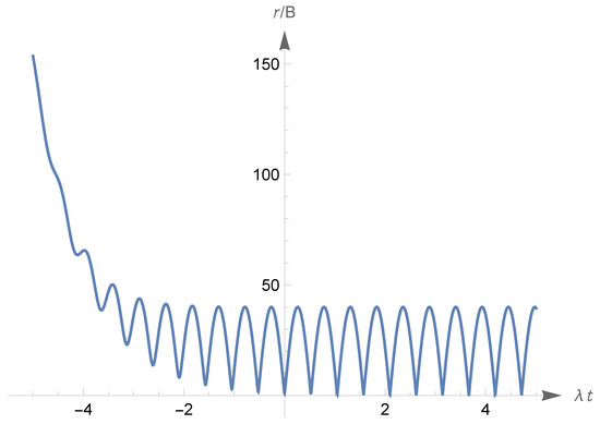
Figure 31.
With reference to Section 8.11, let , and , with arbitrary . The curve in blue is a graph of the as a function of , for .
For any , we have ⟺ and ⟺ (); consequently, ⟺. We can accept as a time domain for the present cosmological model a (maximal) interval where is never vanishing; we take
Let us also remark that, for the mass density parameter, Equation (461) gives in this case
The radius function is given by
and its derivative reads
where
Let us remark that for all , which implies for all and all ; depending on the values of and , the function does not possess or possesses zeroes in the interval . Consequently, for all , the following holds:
while the function does not possess or possesses zeroes in the interval , depending on the values of the ratios and ; if such zeroes exist, we can say that the radius oscillates for t in a right neighborhood of 0. Finally, let us remark that
Similar conclusions hold for the scale factor (), given by (335); vanishes for , thus presenting a Big Bang, and grows exponentially for . The present cosmological model is past timelike and lightlike singular since it violates conditions (65) and (66); it is future timelike and lightlike nonsingular since it fulfills (67) and (68).
In Figure 32 and Figure 33, we describe the curve and the radius for a specific choice of the parameters giving rise to zeroes of , i.e., to initial oscillations of the radius.
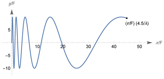
Figure 32.
With reference to Section 8.11, let , , and , with arbitrary . The curve in blue is the range of the map for . We have indicated the point for ; also, let us recall that for .
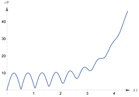
Figure 33.
With reference to Section 8.11, let the parameters be fixed as in Figure 32. The curve in blue is the graph of as a function of the variable , for .
9. Concluding Remarks
In the present work, we discussed the FLRW cosmologies with perfect fluids and a scalar field, paying special attention to some exactly solvable models with a phantom scalar. In spite of the rich literature on FLRW cosmologies with scalar fields, we think there are chances to further individuate exactly solvable models or, at least, to classify more exhaustively the already known solvable cases, especially in the presence of a phantom scalar; in the phantom case with a periodic self-potential, the mechanical analogy with a particle in a Euclidean plane, emphasized in Section 7, might offer a guidance in these investigations.
Author Contributions
M.C., M.G. and L.P. contributed equally to all aspects of this article. All authors have read and agreed to the published version of the manuscript.
Funding
This work was supported by: INdAM, Gruppo Nazionale per la Fisica Matematica; INFN, projects MMNLP and BELL; MUR, project PRIN 2020 “Hamiltonian and dispersive PDEs”; Università degli Studi di Milano.
Data Availability Statement
The original contributions presented in this study are included in the article, further inquiries can be directed to the corresponding author.
Acknowledgments
We are grateful to the funding institutions mentioned above, and to Davide Fermi (Politecnico di Milano) for encouraging us to undertake the present investigation. We are also grateful to all the reviewers of the present work; their comments yielded improvements in the presentation of our results.
Conflicts of Interest
The authors declare no conflicts of interest.
Appendix A. Riemannian Manifolds, Spacetimes, and Dimensional Analysis
Let us repeat the convention Section 2.2: all manifolds considered in this paper are real, smooth, Hausdorff, connected and paracompact.
Let denote any manifold of dimension . A Riemannian metric on is usually described as a smooth map h assigning for each an inner product . In the present paper, for consistency with the dimensional analysis aspects introduced in Section 2.1, we must accept a minimal change in the conventional viewpoint and assume where is the real, one-dimensional, oriented vector space of lengths (thus, each tangent vector has a squared norm and a norm in the semi-space of non-negative lengths)42. The pair will be indicated as a Riemannian manifold. Let us recall the traditional denomination of “squared line element” for the map sending a tangent vector (at any point) to ; for any coordinate system of in which h has coefficients , we can write .
Let us now consider a manifold of dimension , where . Our definition of a Lorentzian metric g on takes into account the same dimensional aspects: so, g is a smooth map assigning for each a symmetric nondegenerate bilinear form of signature . The pair will be referred to as a Lorentzian manifold, or a spacetime; d will be called the spatial dimension. A tangent vector X (at any point ) will be called timelike, lightlike or spacelike in the three cases , or (of course, is short for ). We will employ the traditional denomination of “squared line element” for the map sending a tangent vector X (at any point) to ; of course for any coordinate system of .
Remark: In the present appendix and in the subsequent Appendix B, Appendix C, Appendix D and Appendix E, we primarily use an intrinsic language, in which index notation has just an ancillary role; this style is suitable for the treatment of some technical issues. The use of indices is preferred in Appendix F and in the main text of the paper; however, many formulas therein can be interpreted via the abstract index notation of Penrose [45,82], which is in fact equivalent to the intrinsic, index-free language.
Appendix B. FLRW Spacetimes and Generalizations
For subsequent use, let us recall from Section 2.1 that the real, one-dimensional, oriented vector space is identified with in our setting where the speed of light is .
The spacetime manifold and its metric. For , let us consider the product manifold
where is an open interval with its natural coordinate , and is any manifold of dimension d. A coordinate system of is generically indicated with (with Latin indexes).
We assume that carries a Riemannian metric h, and that a (smooth) function , is assigned. With these ingredients, we can define a Lorentzian metric g on in the following way: for each and for any pair of tangent vectors , in the tangent space , one has
(in the sequel, we often reproduce this equation by omitting the subscripts and S). A more traditional description, in terms of the squared line elements corresponding to g and h, is
A spacetime of this kind is introduced in Section 3.1 (see Equations (15) and (17)) with specific prescriptions for the Riemannian manifold , which is assumed to be complete (see Appendix D) and with constant sectional curvature; in this case, as in Section 3.1, we refer to an FLRW spacetime.
On the contrary, in the present appendix, the Riemannian manifold is unspecified; in the absence of this specification, a spacetime of the form (A1) and (A2) is referred to as a generalized FLRW spacetime.
Let us consider any coordinate system of ; this induces the following coordinate system on the generalized FLRW spacetime :
(here and in the sequel, Greek indices always range from 0 to d). In these coordinates, the spacetime metric g has coefficients , where
(these facts were already noted in Section 3.1 for usual FLRW spacetimes).
Curves in a generalized FLRW spacetime. In the sequel, we frequently consider curves in a spacetime of this kind; it is convenient to fix some notations and write down some equations to be cited subsequently. A (parametrized) curve in a generalized FLRW spacetime is a map
The velocity of at any is
Due to (A2), we have
and one easily infers from here when the velocity is timelike, lightlike or spacelike.
Christoffel symbols, Ricci tensor, and scalar curvature in a generalized FLRW spacetime. Given a spacetime of this kind, we consider the connection induced by the metric g, and we employ a coordinate system as in Equation (A4).
Let us compute in these coordinates the Christoffel symbols of the metric connection; the standard rule and Equation (A5) give
where ∘ (as in Section 3.1), and are the Christoffel symbols in coordinates of the connection on induced by h (in Appendix E, we will use the above expressions to discuss geodesic curves in a spacetime of this kind).
We now consider the Ricci tensor and the scalar curvature R of g; the usual prescriptions and give in the present case
where and r are the Ricci tensor and the scalar curvature of the metric h.
The case of a usual FLRW spacetime. In particular, we have [71]
Appendix C. Time Orientation of a Spacetime: The Case of a Generalized FLRW Spacetime
Let us consider an arbitrary spacetime , i.e., a -dimensional manifold () equipped with a Lorentzian metric g.
For any , the set of timelike tangent vectors at has two connected components, each one formed by the opposites of vectors in the other component. A time orientation of is a rule assigning smoothly for each one of these two components, denoted with and called the future at ; the other connected component (i.e., the set of opposites ) is called the past at . The expression “smoothly” used before must be intended as follows: for each , there is a smooth vector field X defined on an open neighborhood of , such that for each .
Depending on the spacetime considered, it may be possible or impossible to assign smoothly for all [12]; in these two cases, we speak, respectively, of a time-orientable or non-time-orientable spacetime. In the orientable case, there are just two time orientations: if is one of them, the other one is the correspondence .
A time-oriented spacetime is a spacetime , equipped with a time orientation . Given such a structure, a timelike tangent vector at is said to be future-directed or past-directed, if it belongs to or to ; a lightlike tangent vector is said to be future-directed or past-directed, if it belongs to the boundary of , or to the boundary of (in the natural topology of the tangent space at ). To continue, let us consider in a (parametrized) curve, i.e., a smooth map
with an open interval. Assume that, for each , the velocity is timelike or lightlike; in this case we define to be future-directed, or past-directed, if such feature is possessed by the velocity at any .
The case of a generalized FLRW spacetime. Let us consider a generalized FLRW spacetime (), for which we keep all notations of Appendix B; in particular, indicates an open interval in the one-dimensional, oriented vector space of times and a tangent vector at is represented as a pair .
This spacetime carries a natural time orientation, in which the future at any point is
the boundary of the future is
The past and its boundary have similar descriptions, with the inequality replaced by .
We now consider a (parametrized) curve in this spacetime, for which we use the representation (A6) , ( is an open interval); this has velocity as in Equation (A7). On the grounds of Equation (A14), if the velocity at is timelike, we have the equivalence
if the velocity at p is lightlike, due to (A15), we have
Appendix D. A Review on Geodesics and Several Associated Notions of Completeness, Mainly in Riemannian Manifolds and in Spacetimes. Nonsingular Spacetimes
Geodesics in a manifold with connection, and the associated notions of completeness. Let us consider a manifold (of any dimension m); a (parametrized) curve in is a smooth map
with an open interval. From now on, we assume to carry a connection and denote with ∇ the corresponding covariant derivative. Given a curve as above, we can define the velocity
and the acceleration
If is a coordinate system of , the curve has a coordinate description 43. Of course, the velocity of has components ; the acceleration has the following components:
where are the Christoffel symbols of the connection. is said to be a (parametrized) geodesic if
(everywhere on the interval ).
A geodesic is said to be maximal if it cannot be extended to a geodesic , defined on an open interval that contains properly. A geodesic is said to be complete if (which, of course, implies to be maximal).
The manifold with connection is said to be geodesically complete if every maximal geodesic is complete.
The case of a Riemannian manifold. All the notions introduced in the previous paragraph apply, in particular, to the case of a Riemannian manifold , with the connection induced by the metric h; it is well known that
Moreover, the completeness of in the geodesic sense of the previous paragraph can be shown to be equivalent to the usual completeness of as a metric space, with the distance induced by h44.
The case of a spacetime. We now consider a spacetime (i.e., a manifold equipped with a Lorentzian metric), and the connection induced by g. A result analogous to (A23) holds, namely
In the present framework, one can refine the notion of geodesic completeness by distinguishing among timelike, lightlike and spacelike geodesics45; further refinements are possible if is equipped with a time orientation, allowing us to distinguish between future-directed and past-directed geodesics of the timelike or lightlike type.
Assuming a time orientation is given, let denote a future-directed, timelike, or lightlike geodesic in , defined on an open interval . We say that is past complete if , and future complete if .
The time-oriented spacetime is said to be:
- Past timelike complete if each maximal, future-directed timelike geodesic is past complete;
- Past lightlike complete if each maximal, future-directed lightlike geodesic is past complete;
- Past complete if it is both past timelike and past lightlike complete.
The notions of future timelike complete, future lightlike complete, and future complete spacetime are defined similarly, requiring the future completeness of maximal, future-directed geodesics. A spacetime is said to be timelike complete, lightlike complete, or complete if it possesses the previous properties both in the past and the future (i.e., for the maximal geodesics of the corresponding types).
The adjective nonsingular is often used as an equivalent for “complete. So, we can say that a spacetime is past timelike nonsingular, past lightlike nonsingular, ⋯, timelike nonsingular, lightlike nonsingular, nonsingular.
Needless to say, the terms incomplete and singular will be used as negations of “complete” and “nonsingular”.
Appendix E. Geodesics and Geodesic Completeness of Generalized FLRW Spacetimes
Let us consider a generalized FLRW spacetime (), for which we keep all the notations of Appendix B; in particular, g is the metric of and h the (Riemannian) metric of (see Equation (A2)). We equip this spacetime with the time orientation described in Appendix C. In addition, we prescribe the following:
(using in both cases the metric connections).
Curves in : reminders, and computation of the acceleration. Let us consider a (parametrized) curve in ; as already indicated in Appendix C, this is a map of the form (A6), here reproduced,
Let us also recall Equations (A7) and (A8) (here rephrased as equalities of functions, holding everywhere on )46:
In the sequel, and will be referred to as the “squared velocities” of the curves and . Using the covariant derivative ∇ in (A25) we can also define the acceleration , which is computed hereafter.
Let us consider a coordinate system as in Equation (A4); in these coordinates, the curve has a description , given by
where, of course, (for all p such that is in the domain of the coordinates ). Equations (A21), (A9) and (A28) give
where (we repeat it) are the Christoffel symbols of the metric connection on . In intrinsic language, this means that
(let us recall that D is the covariant derivative in , see (A25); needless to say, in the above A is a scalar function on the interval , while B is a function from the interval to the tangent bundle of , given by the acceleration of the curve plus a correction depending on ).
Curves in : new expressions for the squared velocity and for the acceleration, upon a reparametrization of the component in . Let us consider any curve , for which we keep all notations of the previous paragraph. Following a hint by O’Neill [60] we reparametrize the second component of introducing the map
We note that is smooth and, for all ,
thus, is an open interval in , and is a diffeomorphism between and . Due to these facts, there is a unique smooth map
This is clearly a reparametrization of the curve ; in the sequel, we write the above equation as . In the same style, we can write
inserting this result into Equation (A27) and into the first equality (A32), we obtain
Let us recall that the pair gives the acceleration of , see Equation (A31).
Characterization of geodesics in . Let us again consider a curve
According to the results in the previous two paragraphs, we can uniquely represent as
with as in (A33), and
( smooth; we recall that are open intervals, and is a smooth diffeomorphism). Let us recall that the squared velocity of has the expression (A37), and the acceleration of is given by Equation (A31), with A and B as in Equations (A38) and (A40). That said, we have the following equivalences:
On the grounds of general results, already mentioned in Appendix D, the geodesic nature of and implies the constancy of the corresponding squared velocities, which are related through Equation (A37). Putting together the previous considerations, we obtain the following:
Let us note that are in the space of squared lengths (which is the range of h and g; see Appendix A). After introducing for each the potential function
we can rephrase Equation (A45) in the following way:
Let us note that
and that, if is timelike or lightlike, it is future-directed under the conditions (A16) and (A17).
The equations and are the law of motion and the conservation law of energy of a fictitious one-dimensional, conservative mechanical system with kinetic energy and potential energy .
Let us assume the conditions (A47) to be fulfilled by . Then, we have the following statements, which are used in the next paragraph:
The maximal geodesics in in terms of their Cauchy data, assuming completeness of . We again consider a generalized FLRW spacetime (), for which we use all previous notations; in addition, we represent the open interval in terms of its endpoints, i.e.,
From now on, we assume that
Let us define a Cauchy datum (more briefly, a datum) as an ordered set
Given such a set, let us denote with
(with ) the maximal geodesic in such that
Of course, any maximal geodesic in has the form , for some datum ♭ as above. On the grounds of the description of the geodesics in the previous paragraph, for each datum ♭, we have
where47:
Again due to the results in the previous paragraph, we have
(the expression for follows computing the above constant function at ). Of course,
Referring once more to the previous paragraph, we see that
if we also take into account Equations (A16) and (A17), we find
(note that and ⟺ ⟺ constant). In addition,
(In the above, the endpoints are always determined by requiring to be maximal among the solutions with values to ; in cases with described above, maximality is equivalent to requiring , and a similar statement with and interchanged holds in the above cases with ).
Completeness conditions for generalized FLRW spacetimes. The necessary and sufficient conditions for a generalized FLRW spacetime to be lightlike complete were obtained by O’Neill [60] (see Chapter 12, Remark 27). Sanchez derived in [62] the necessary and sufficient conditions for a generalized FLRW spacetime to be complete both in the timelike and in the lightlike sense, on the grounds of more general results by Romero and Sanchez for warped product spaces [61]. Hereafter, we report the results of [60,62], which are accompanied by the corresponding proofs just to make the present exposition self-contained. The proofs presented here follow the arguments in the cited works, with some adaptation to our language (concerning, e.g., our use of the spaces of times and lengths).
Throughout this paragraph, we consider a generalized FLRW spacetime (), for which we maintain the notations and assumptions of the previous paragraph; in particular, we use the representation (A52) and the completeness assumption (A53) for the Riemannian manifold . Appendix D is our reference for all completeness notions mentioned here and in the sequel in relation to or to .
Proposition A1.
- (i)
- is past timelike complete if and only ifIf all maximal, future-directed timelike geodesics are past incomplete. If and all maximal, future-directed timelike geodesics with nonconstant projection on are past incomplete.
- (ii)
- is past lightlike complete if and only if(note that (A69) does not require to be ).If all maximal, future-directed and nonconstant lightlike geodesics are past incomplete.
- (iii)
- is future timelike complete if and only ifIf all maximal, future-directed timelike geodesics are future incomplete. If and all maximal, future-directed timelike geodesics with nonconstant projection on are future incomplete.
- (iv)
- is future lightlike complete if and only if(note that (A71) does not require to be ).If all maximal, future-directed and nonconstant lightlike geodesics are future incomplete.
Proof.
which proves the integral in (A68) to be .
(the above integral from to equals again due to (A68); the other integral converges).
(note that, with our assumptions, both integrals above are convergent).
We will present the proofs of (i) and (ii), organizing them in several steps; the arguments proving (iii) and (iv) are very similar and will not be discussed.
Let us note that the definition of past timelike completeness in Appendix D is equivalent, with the notations of the previous paragraph, to the following statement:
Similarly, the notion of past lightlike completeness in Appendix D is equivalent to the following statement48:
Step 1. Equation (A72) (past timelike completeness of ) implies Equation (A68). Assuming (A72), we first consider a datum ♭ as in (A54) with , and , so that ( = constant and) . Then, , so ♭ has the form considered in (A72). From (A72), we know that ; on the other hand, Equation (A66) tells us that , so
this is the first statement in Equation (A68). In order to prove the second statement in (A68) (i.e., the divergence of the integral therein), we choose a datum ♭ as in (A54) with , , (implying ) and ; from the expression of and from (A61), we infer . Since , Equation (A72) tells us that . On the other hand, has the expression provided by the last lines in Equation (A67) with the present specifications for , , , and we already know that ; thus
Step 2. Equation (A68) implies Equation (A72) (past timelike completeness). Assuming Equation (A68), let us consider any datum ♭ with and ; our aim is to prove that .
If , according to the last lines in Equation (A67), we have
Step 3. If , all maximal future-directed timelike geodesics are past incomplete. Assuming , let us consider a maximal, future-directed timelike geodesic; this will be of the form for some datum ♭ with , . Hereafter, we will show that .
Indeed, if , according to Equation (A66), we have
Step 4. If and all maximal, future-directed timelike geodesics with nonconstant projection on are past incomplete. With the given assumptions, let us consider a maximal, future-directed timelike geodesics with nonconstant projection on ; this will be of the form for some datum ♭ with , and ( is impossible since this would imply constant, against the assumption of nonconstant projection on ). Hereafter, we will show that .
Indeed, according to the last lines in Equation (A67), we have
Step 5. Equation (A73) (past lightlike completeness) implies Equation (A69). Assuming (A73), we choose a datum ♭ as in (A54) with , , (implying ) and ; from the expression of and from (A61), we infer . Since , and , Equation (A73) tells us that . On the other hand, has the expression provided by the last lines in Equation (A67) with the present specifications for , , ; thus,
which proves the integral in (A69) to be .
Step 6. Equation (A69) implies Equation (A73) (past lightlike completeness). Assuming Equation (A69), let us consider any datum ♭ with , and ; we aim to prove that .
Indeed, according to the last lines in Equation (A67), for the datum under consideration, we have
(the above integral from to equals due to (A69), and the other integral converges).
Step 7. If all maximal, future-directed and nonconstant lightlike geodesics are past incomplete. Assuming convergence of this integral, let us consider a maximal, future-directed and nonconstant lightlike geodesic; this will be of the form for some datum ♭ with , and (let us recall Equation (A65); the case , mentioned therein is impossible, since it would imply constant). Hereafter, we will show that .
Indeed, applying the last lines in Equation (A67) to the present datum, we obtain
(since, with our assumptions, both integrals above are convergent). □
Appendix F. A Review the Energy Conditions
Let us consider a spacetime of dimension with ; the present appendix follows [12] for the case , and [13] for arbitrary d.
Let us assume that a (symmetric) stress–energy tensor has been specified at a spacetime point (which is fixed in all the subsequent discussions). The stress–energy tensor is said to fulfill the weak energy condition (WEC) if
The stress–energy tensor is said to fulfill the strong energy condition (SEC) if
(The following should be noted: if the Einstein equations hold, with as in Section 2.2, we have ; in this case, the SEC is equivalent to for each timelike tangent vector , which is the condition typically considered in the singularity theorems of Penrose, Hawking, and Geroch mentioned in the Introduction.)
References [12,13] discuss other energy conditions, the most important being the dominant energy condition (DEC); these will not be considered in the present paper.
To continue, let us recall that a basis of tangent vectors () is called orthonormal if for where , for and for 49. That said, assume one can associate an orthonormal basis with the stress–energy tensor such that the matrix
has the diagonal form
In this case, it can be shown that [13]
In particular, assume that the stress–energy tensor has the perfect fluid form
In this case, we can set and add to this vector other vectors () so as to obtain an orthonormal basis. The matrix elements of with respect to this basis have the form (A77), with as in (A80) and
thus, for all a, , and the equivalences (A78) and (A79) assume the forms (52) and (53) reported in the main text.
Appendix G. On the Determination of the Fluids’ Densities
Proof of the equivalence (102) (under the assumption (101)). As in Section 4.1, let us choose arbitrarily a smooth function , (with an open real interval), and consider any smooth function , .
If for some , computing and using the expression in (100) for , we readily obtain Equation (84) with .
Conversely, assume fulfills (84) with , choose and let be such that (such a function exists due to (101)). Let us provisionally put . Then, (using again the expression for in (100)), we see that , with ; moreover, (by the previous choice for ) . To summarize, and fulfill the same ODE and coincide at time : so, by the standard uniqueness theorem for the Cauchy problem, we have .
On the quadrature formula (105) (under the assumption (104)). This quadrature formula arises in an obvious way from the differential equation for in (100) and from the specified initial condition . Let us show that (105) actually individuates a smooth function .
For this purpose, let us recall that the first condition in Equation (104) reads for all whence, by continuity, = constant . To continue, let us rephrase Equation (105) as
By construction, the function is smooth with never vanishing derivative , of constant sign equal to . Again due to (104), for and for ; thus, is a smooth diffeomorphism between and . On the other hand, the map is also a diffeomorphism between and ; so, the condition in (A82) actually defines a unique smooth function .
Appendix H. Comparing the Zero Energy Motions of Two One-Dimensional Lagrangians
Let us consider, in general, two smooth Lagrangians
related by
where is a smooth, never vanishing function. The corresponding energy functions are , , and it is readily seen that
Let us now show that the zero-energy solutions of the Lagrange equations induced by and coincide. In fact, along any function , we have
this identity, with the relation (A85) between and with the assumption that g never vanishes, ensures the following: a function fulfills , if and only if it fulfills , .
Appendix I. The Descartes’ Rule of Signs
Some statements in the subsequent appendices are proved via Descartes’ rule of signs (see, e.g., [84]); let us summarize this rule, which allows us to evaluate the number of positive roots of a real polynomial.
We consider a real polynomial function of arbitrary degree, which we represent in terms of its nonzero coefficients arranging in increasing (or decreasing) order the corresponding powers:
Let us consider the list of nonzero coefficients and the list of their signs (i.e., for ). Let C be the number of sign changes between consecutive terms in that list (i.e., ).
Then, the number of positive roots of (counting each root according to its multiplicity) is , for some even integer P such that .
Appendix J. Two Statements on a Class of Polynomials
Let
We introduce the polynomial function
(noting that any polynomial of the form , with , can be represented as above with ). We also set
(noting that is nonempty; from now on, any sum over is meant to be zero if is empty).
The forthcoming statements (i) and (ii) individuate two special values and , with suitably defined, such that and ; these results will be employed in some of the subsequent appendices to locate the zeroes of certain polynomials of the form (A88) and (A89). Here are the two statements, which are proved in the sequel of the present appendix:
- (i)
- LetThen, is well defined, and
- (ii)
- In addition, assumeand putThen, is well defined, and
Proof of (i). Let us consider Equation (A91) defining , and note that ; in fact , , for all and for some . Thus, the term between round brackets in Equation (A91) is ; this suffices to infer that the quantity therein is well defined and fulfills (A92).
However, for any we have since and ; since for all and for some , this implies for all , with a strict inequality < for some k. Thus
and the term between square brackets vanishes due to the definition (A91) of ; so, the relation (A93) is proved.
Proof of (ii). Let us consider the ratio defining in Equation (A95). The numerator in this ratio is positive due to (A94), and the denominator is positive since and for all . Thus, is well defined and . Moreover,
(since ); thus, , and the proof of (A96) is concluded.
Let us proceed to prove Equation (A97); for this purpose, we write
Since , and for all , by Bernoulli’s inequality (see, e.g., [85]), we have and for all . Since , for all and for some , we infer
Let us also note that for and for , so that
Appendix K. Proof of Statements (185) and (186) on the Potential of the Standard Cosmological Model
We consider the potential of (183), with the assumptions (165) and (176) and with an unspecified sign for ; let us derive the results (185) and (186) about the derivative . For this purpose, we note that Equation (183) implies
where we have introduced the polynomial function
Equation (A106) implies that, for all ,
Let us discuss the zeroes of in , using their coincidence with the positive roots of the polynomial and employing Descartes’ rule of Appendix I. The nonzero coefficients of are , with signs . The number of sign changes in this list is ; the number of positive roots of is with even and , which means . In conclusion, there is a unique such that
this is also the unique zero of in , described by Equation (185). The function is never vanishing on and on ; hence, by continuity, has a constant nonzero sign on each one of these intervals. On the other hand, for , we have , while for , we have ; these facts suffice to infer
Appendix L. Proof of Statements (a)–(d) in Section 6.5 about the Function of Equation (201)
Let us recall the general assumptions (198)–(200) and (204); the proofs of (c) and (d) also require condition (211).
Of course, (A111) implies that, for all ,
Keeping in mind these facts, let us discuss the positive roots of the polynomial using Descartes’ rule reviewed in Appendix I. If the nonzero coefficients of are with signs ; if the nonzero coefficients of are with signs . In both cases, the number of sign changes is and the unique number of the form , with even and , is .
In conclusion, there is a unique such that
this is also the unique zero of in , described by Equation (205). The function is never vanishing on and on ; hence, by continuity, has a constant nonzero sign on each one of these intervals. On the other hand, for , we have , while for , we have ; these facts suffice to infer
Due to (A113), the reversed inequalities hold for in these two intervals; this proves statements (206).
Finally, let us prove the inequality (207) . Due to (A114) and (A115), it will suffice to show that
in fact, Equations (A112) and (200) give51
Proof of (b). It is evident that the quantities defined by (208) fulfill and . That said, let us derive the lower and upper bounds (209) on ; for this purpose, we apply the general setting of Appendix J, choosing for the polynomial function of Equation (A112). By comparison between Equations (A88), (A89) and (A112), we see that in the present case
Due to (A118), Equations (A91) gives in the present case
with as in (208); the condition (A94) is automatically fulfilled, and Equation (A95) gives
with as in (208).
By comparison between Equations (A121), (A114) and (A115), we obtain and ; these are just the bounds on in (209) (and it is evident that the upper bound implies a less refined bound ).
Proof of (c). Equation (210) tells us that
where we have introduced the polynomial function
of course (A122) implies that, for all ,
Let us discuss the zeroes of in , using their coincidence with the positive roots of the polynomial and employing again Descartes’ rule of Appendix I. The nonzero coefficients of are , with signs . The number of sign changes in this list is ; the number of positive roots of is with even and , which means either or .
We now show that has in fact two distinct, positive roots using the inequality (211) , which is assumed in (c). In fact,
and the above term between round brackets is positive due to (211), so that
On the other hand, from the definition of , it appears that
Thus, there is a unique pair such that
moreover,
Since has the same zeroes and the same sign of on , statements (212) and (213) of (c) about the zeroes and the sign of are proved. Moreover, Equation (A128) gives the second and the third inequality in (214).
To conclude, let us prove the first inequality in (214), namely the relation
Due to the already proved statements (205) and (206) in (a), to obtain the inequality (A130), it suffices to show that
on the other hand, we know that and that on ; thus, and, consequently, (A131) follows if we show that
Proof of (d). It is evident that the quantities defined by (215) fulfill , (by (211)) and . That said, let us derive the lower and upper bounds (216) on ; for this purpose, we apply the general setting of Appendix J, choosing for the polynomial function of Equation (A123). By comparison between Equations (A88), (A89) and (A123), we see that in the present case
Due to (A135), Equations (A91) gives in the present case
with as in (215). The condition (A94) is fulfilled, since
and the above quantity is positive due to the assumption (211). Equation (A95) gives
with as in (215). The inequality (A93) becomes in this case
On the other hand, the inequality (A140) cannot hold; in fact, if (A140) were true we would infer (because ), while we know from Equation (214) that . Having excluded (A140), we conclude that (A139) holds.
We now refer to the inequality (A97), which in the present case becomes
Appendix M. Proof of Statements (f)–(i) in Section 6.5 about the Function of Equation (220)
Let us recall once more the general assumptions (198)–(200) and (204); the proof of (i) also requires condition (211).
Let us discuss the zeroes of in using their coincidence with the positive roots of the polynomial , and employing again Descartes’ rule of Appendix I. If , the nonzero coefficients of are , with signs ; if , the nonzero coefficients of are , with signs . In both cases, the number of changes in the list of signs is ; the number of positive roots of is with even and , that means .
Thus, there is a unique such that
Noting that for and for , we also infer
Equations (A144)–(A146) yield statements (226) and (227) in (f) about the zero and the sign of . The statements in (f) after Equation (227), yielding Equations (228) and (229), are obvious.
Proof of (g). It is evident that the quantities defined by (230) fulfill and . That said, let us derive the lower and upper bounds (231) on ; for this purpose, we apply the general setting of Appendix J, choosing for the polynomial function of Equation (A143). By comparison between Equations (A88), (A89) and (A143), we see that in the present case
Due to (A147), Equations (A91) gives in the present case
with as in (230); the condition (A94) is automatically fulfilled, and Equation (A95) gives
with as in (230).
By comparison between Equations (A150), (A145) and (A146), we obtain the inequalities (231) about ; the comment in (g) after Equation (231) is obvious.
Proof of (h). We must derive the bounds (232) and (233) on , on the grounds of the bounds (231) on . For this purpose, let us rephrase the definition (220) of for all as follows:
This holds, in particular, for (note that, for any and in particular for , we have due to (224), and this ensures the positivity of the factor between square brackets in the right-hand side of Equation (A151)). On the other hand, due to (231), we can write
and
i.e.,
again due to (231), we have
Using Equation (A151) with , and inserting therein the inequalities (A152)–(A154) we readily obtain the bounds (232) on , with and as in (233).
Proof of (i). Assume (211) holds. Our aim is to infer the inequality (235) under the supplementary condition (234) . For this purpose, we use the known inequalities
(see the comment after Equation (231) and Equation (216)). Due to these relations, we have if
on the other hand, (A156) is clearly equivalent to (234).
Appendix N. Proof of Equation (250) (Including Convergence of an Integral Therein)
Let us keep the assumptions (198)–(200), (204), (211) and (234) of Section 6.6; as in Equation (247), we refer to the time such that . From now on, we consider any time such that
(so that ). Using, e.g., Equation (148) we can write
On the other hand,
In the last expression above, the second integral equals due to (A158); the first integral will be denoted with . To summarize,
Of course, this implies
We now consider the limit ; then , and
Appendix O. Proof of Some Statements about in Equation (271)
Equation (271) involves the polynomial function
and states that has a unique root in , indicated with ; the same equation states that, for , if and only if . The subsequent Equations (272) and (273) contain inequalities about . All these claims are proved hereafter.
Proof that has a unique root in . We again use Descartes’ rule of Appendix I. The nonzero coefficients of the polynomial are , with signs . The number of sign changes in this list is ; the number of positive roots of is with even and , which means . To summarize, there is a unique such that
The sign of on . Clearly, has a constant nonzero sign on each one of the intervals and . Noting that for and for , we conclude that
Proof of the relation (272) . Let us consider besides the polynomial function of Equation (A112). We have
from here and from , we obtain
Proof of the bounds (273) on . We apply the general setting of Appendix J, choosing for the polynomial function of Equation (A166). By comparison between Equations (A88), (A89) and (A166), we see that in the present case
Appendix P. A Usefulf Inequality
In the sequel, we prove (A175); our argument will be divided into two steps.
Step 1. One has
To prove this, let and . By the Bernoulli inequality (see again [85]), for any , we have . In addition, if ; thus,
To continue, we note that for all . If we also have , so that ; equivalently, we can say that
Finally, for , i.e.,
Appendix Q. Estimates on the Time in Equation (244)
Let us again refer to the potential of Equation (201), under the assumptions (200) and (204). We consider a time by admitting the integral representation (244)
where is the unique zero of , and the final extreme in the integral is any real number such that .
In the sequel, we will derive rigorous upper and lower bounds for , and we will present situations in which they are useful to estimate .
Statement of the bounds on . Let us define the constants
(noting that and ); moreover, let us introduce the functions
That said, our bounds on are as follows:
The inequalities in (A183) have a general validity, but of course they deserve a special interest when and are close. From the explicit expressions of , it is clear that are close if , and is not large, which happens if are both small and is not large.
The forthcoming three paragraphs in this appendix will be devoted to the proof of (A183). The subsequent paragraph will present coarser bounds on , following from (A183) when lower and upper bounds are available for and . The final two paragraphs will describe a number of applications; these include the justification of Equations (285)–(287) in the main text, describing the asymptotic behavior of certain times when the parameter of Section 6.4, Section 6.5 and Section 6.6 is sent to zero.
A preliminary to the derivation of (A183): a new integral representation for . According to Equations (A111) and (A112), for all , we have
from Equations (A114) and (A115), we know that and for all . Equation (244) for can be rephrased as
Let . By the Taylor formula, we have
These facts will be used hereafter to derive the lower and upper bounds (A183) on .
Proof of the lower bound in (A183). Keeping in mind Equations (A184)–(A187) we note that, for ,
with as in Equation (A180). Again for , Equations (A185), (A186) and (A188) give
and inserting this inequality in (A184), we obtain
We now reexpress the last integral via a change in variable , . By comparison with the definition (A180) of , we can write equivalently and this gives
We finally expand , and integrate term by term; by comparison with Equation (A182), this gives the lower bound on in Equation (A183).
Proof of the upper bound in (A183). We refer again to Equations (A184)–(A187). Let ; noting that Equations (A186) and (A187) imply
we infer from (A185) that
Inserting this inequality into Equation (A184), we obtain
We now reexpress the last integral via a change in variable , , which gives
Expanding , integrating term by term and comparing with Equation (A182), we finally obtain the upper bound on in Equation (A183).
Coarser bounds on , following from (A183). We now assume that we have bounds and for and , fulfilling the inequalities
In this case, let us put
(noting that and ). We claim that the time described by Equation (244) admits the bounds
where () are again the functions in (A182).
In order to prove (A200) we start from the bounds (A183) , where are defined via the functions and the constants of Equation (A180). It is readily checked that , , , and that is (strictly) decreasing for . These facts (and the inequalities ) imply
so the bounds (A200) follow from the bounds (A183), of which they are coarsenings. Needless to say, the coarser bounds (A200) are especially interesting when and in Equation (A197) are sufficiently close to and , respectively.
Applications of the coarser bounds (A200). Let us make the assumptions (200), (204), (211) and (234). The bounds (A200) can be applied to the times in Section 6.5, Section 6.6 and Section 6.7 with , using available bounds and (that are required to fulfill (A197)).
More precisely, we can use the bounds provided by Equations (208) and (209), and the bounds provided by Equations (230) and (231) for , by Equations (215) and (216) for , and by Equation (273) for (i.e.: and , with as in Equation (208); with as in (230), and so on).
Justification of the asymptotic expressions for certain times. Let us consider a family of models as in (217), and the limit . In the main text, it is stated that the times () have the asymptotic expressions (285), (286) and (287) for .
Appendix R. Further Estimates on the Time in Equation (244)
Let us refer once more to the potential of Equation (201), under the assumptions (200) and (204); we reconsider the quantity in Equation (244), with . In the present appendix, we will derive upper and lower bounds on , different from those of Appendix Q, and we will illustrate situations in which the new bounds are useful.
Statement of the bounds on . We begin our construction by introducing the constants as in (A180), and
(note that and ); from these objects, we build the function
That said, our bounds on are
The inequalities in (A204) have a general validity but, of course, are especially useful when the bounds are close. It is seen from the explicit expressions that and tend to the same limit if is sent to while keeping and the other parameters fixed; this suggests that and should be close for small and for appropriate values of and of the parameters, a fact that is checked a posteriori in many interesting cases and, in particular, in the applications of the present framework considered in Section 6.7.
In order to employ the bounds (A204), the integral appearing therein must be computed numerically; however, this calculation is more reliable than the direct numerical computation of via (244), due to the nonsingular nature of the function on .
The forthcoming three paragraphs in this appendix will be devoted to the proof of (A204). The subsequent paragraph will present coarser bounds on , following from (A204) when suitable bounds are available for and ; the final paragraph will describe a number of applications.
A preliminary to the derivation of (A204): another integral representation for . We start from the representation (A184)
where is the polynomial function defined in Equation (A112). Having degree 6, the polynomial coincides with its Taylor expansion of order 6 about any point and, in particular, about ; thus, for all real , we have
From Equation (A186), we know that and , with as in Equation (A180). Moreover, with as in Equation (A202), we have
Thus, for all real ,
We insert this expression for into Equation (A184), and then we reexpress the integral therein via a change in variable , . In this way, we obtain
with as in Equation (A203). The integral representation (A208) will be used hereafter to derive the lower and upper bounds (A204) on .
Proof of the lower bound in (A204). Our argument will refer to the inequality
this is just the relation (A175) with .
On the other hand, from the definition (A203) of , it is evident that ; thus, for , we have
Again for , we have of course ; inserting this inequality and the relation (A210) into Equation (A208) for , we infer
this is just the lower bound on in Equation (A204).
Proof of the upper bound in (A204). Let us expand the square in Equation (A208); in this way, we obtain
Now, we insert in the first two integrals above the bound , while we put in the third integral the bound . In this way, we obtain the inequality
which in fact coincides with the upper bound in (A204).
Coarser bounds on , following from (A204). We now assume that we have bounds and , fulfilling the inequalities
In this case, we consider the constants as in (A199), as in (A202) and
(noting that and , ); we also introduce the functions
We now claim that the time in Equation (244) admits the bounds
The comment following Equation (A204) must be rephrased here in the following way: the integrals appearing in (A215) require a numerical calculation which however is more reliable than the direct numerical computation of via (244), due to the nonsingular nature of the functions on .
In order to prove (A215), we start from the bounds (A204) , where are defined via the constants of Equation (A202) and the function of Equation (A203). We have the inequalities , , and for all , which imply
so the bounds (A215) follow from the bounds (A204), of which they are coarsenings. The coarser bounds (A215) are especially useful when and in Equation (A212) are sufficiently close to and , respectively.
Applications of the coarser bounds (A215). Let us make the assumptions (200), (204), (211) and (234). Some interesting candidates for application of the bounds (A215) are the times in Section 6.5, Section 6.6 and Section 6.7 with .
In order to obtain the bounds (A215) for these choices of , we can use available bounds and (which are required to fulfill (A212)). More precisely, we should note the following:
- According to (249), the time corresponds to the value of the scale factor; of course, we can set .
Appendix S. On the Quantity in Equation (292)
Let us refer to the general framework of Section 6.5 and Section 6.6, keeping in mind, in particular, the assumptions (200) and (204). Equation (292) contains the quantity
accounting for the variation in the scalar field from (the time of the Big Bounce) to , or from to ; we already noted that the integral in the definition of is convergent.
Statement of the bounds on . Let us consider the constants in (A180), and in (A202) ( and ); moreover, let us choose any real number such that
In the sequel we will prove that
The lower bound depends on and involves the Gamma function (factorial function) ; the upper bound is independent of . For small , we have , and .
The forthcoming three paragraphs in this appendix will be devoted to the proof of (A218). The subsequent paragraph will present coarser bounds on , following from (A218) and from estimates on . The final paragraph will use such bounds to justify Equation (293) of the main text, which describes rigorously the asymptotics of .
A preliminary to the derivation of (A218): a new integral representation for . Let us express as in Equation (A111), with the polynomial function of Equation (A112); this gives
We expand in terms of powers of following Equation (A207), and then we reexpress the integral in (A219) via a change in variable , . This gives
Proof of the lower bound in (A218) on . Let us recall the inequality (A175), which we apply with and as in (A217); this gives
It should be noted that
due to condition (A217), we have , which ensures convergence of the integral (convergence of is evident). To continue, we observe that for all we have
so that
Again for , the relations give
and the relation gives
Proof of the upper bound in (A218) on . We return to Equation (A220) and insert therein the inequalities
holding for all . This gives
thus yielding the upper bound of Equation (A218).
Coarser bounds on , following from (A218). We now assume that we have for lower and upper bounds , such that
typical choices will be those provided by (209), namely
with as in Equation (208). We also consider the constants in (A199), in (A213) and in (A202) (; ). We claim that
note that and if we use (A236). The bounds (A237) are coarsenings of the bounds (A218) ; in fact, using the inequalities (A235) and , , , we readily see that and .
Appendix T. A More Detailed Description of the Model in Section 6.7
Let us refer to the model in the cited section, based on the choices (302) and (308) for the parameters and .
Appendix U. Proof of Statements (-) in Section 6.8 about the Function of Equation (201)
Proof of () and (). The proofs of all statements in () and () are identical to those of the corresponding statements in items (c) and (d) of Section 6.5: see Appendix L. The cited items (c), (d), () and () refer to the derivative , which is independent of (see Equation (210)); so, the fact that Section 6.5 and Appendix L assume , while Section 6.8 and the present appendix assume , is not relevant for the present discussion.
Proof of (). Let us derive the relation (317) . For this purpose, we use the already-proved inequalities (316) , recalling that is strictly increasing on the interval by (213). Thus
where, in the last two steps, we used the inequalities , and the assumption (314).
Proof of () () () (). First of all, let us show that the parameter defined by Equation (318) is positive; for this purpose, we rephrase Equation (318) as
Of course ; moreover, due to the already proved inequality in (316) we have . In conclusion, .
To continue, let us observe that the definitions (201) of and (318) of ensure
due to (A240), the equivalences (indicated with ⟺) in items () () () are evident. Recalling that behaves as in the already proved statements () and (), it is easy to check all statements in () () () about the zeroes and the sign of , except perhaps for the positioning of in the inequalities (329) of item (). Concerning this issue, let us recall that by (316); it is clear that . We now proceed to compare the quantities ; we know that is strictly increasing on and , while (see (A238)), so we conclude that .
Proof of (). In anyone of cases () () (), we have the following implication for any :
Thus, to prove that , it suffices to show that
Proof of (). Let us refer to the quantities defined by (331). It is evident that . The denominator of in (331) is clearly positive; the numerator is due to (315), so that . Moreover .
We now proceed to prove the bounds (332) on , using an argument rather similar to that employed for proving the bounds (209) (see Appendix L, proof of (b)).
First of all, we represent in the form (A111) for all , where is the polynomial function (A112). Of course, and have opposite signs and the same zeroes in , as stated in (A113). To continue, we apply the general setting of Appendix J, with . By comparison between Equations (A88), (A89) and (A112), we see that in the present case
Due to (A243), Equations (A91) gives in the present case
with as in (331). The condition (A94) is fulfilled, since
(the above statement of positivity is due to (315)). Equation (A95) gives
with as in (331). The inequalities (A93) and (A97) become in this case
i.e., since and have opposite signs,
On the other hand, in anyone of cases ()-() we can say that, for any ,
(to prove this in case (), recall that by (329)). Applying this result with , we obtain . Let us also recall the implication (A241) ⟹; this can be applied with , the conclusion being . In conclusion, both the lower and the upper bound (332) on are proved.
Appendix V. Derivation of Equations (363)–(366)
Let us consider Equation (361) for an unknown function , where ; throughout the present appendix, the term “solution” is employed in relation to (361) to mean a maximal solution. In this appendix, we will show that a function is a solution of Equation (361) if and only if one of the following cases (i)–(iii) occurs:
- (i)
- We have
- (ii)
- We have
- (iii)
- We havewhere(, are the standard norm and inner product of ).
Equations (A250) and (A251) reproduce Equations (363) and (364) in the main text. Equations (365) and (366) in the main text are obtained from (A252) and (A253) renaming the difference . In order to prove that the solutions of (361) coincide with functions of type (i), (ii) or (iii), We proceed in several steps.
Step 1. A function is a solution of Equation (361) if and only if it admits the representation
The above statement is well known (it is just a vector description of the general solutions of equations , ).
Step 2. The solution of Equation (361) with arbitrary initial data , (, ) is unique, and given by
This is another well-known fact.
Step 3. Let () be any solution of (361); then, the function fits case (i) or case (ii), or the following holds:
(iii’) there is such that (with ).
In order to prove the above statements, we start from the representation (A254) of , depending on two vectors . If , case (i) holds; if , case (ii) holds.
We now assume , and infer (iii’). For this purpose, we note that, for all , Equation (A254) implies
where and . Therefore,
and this implies
( is well defined, since ). To summarize, (iii’) holds.
Step 4. Let () be any solution of (361); then (i), (ii) or (iii) holds. To prove this we refer to the third step, ensuring that (i),(ii) or (iii’) holds. We now show that (iii’) implies (iii).
For this purpose, let us consider the derivative . Let be the time mentioned in (iii’), and let us put , ; then,
So, we can express as in (A255), with and orthogonal; due to orthogonality, we can write
Substituting (A260) into (A255), we conclude that the solution can be represented as in (A252) with suitable parameters fulfilling all conditions in (A253). To summarize, (iii) holds.
Step 5. Any function as in (i), (ii) or (iii) is a solution of (361). This is evident.
Appendix W. Derivation of Equations (401) and (402)
Let us consider Equation (399) for an unknown function , where ; throughout the present appendix, the term “solution” is employed in relation to (399) to mean a maximal solution. In this appendix, we will show that a function is a solution of Equation (399) if and only if it has the form
depending on the parameters
(, are again the standard norm and inner product of ).
Equations (A261) and (A262) will justify Equations (401) and (402) in the main text, which are obtained by renaming the difference .
Step 1. The solution of Equation (399) with arbitrary initial data , (, ) is unique, and given by
this implies, among others, that any solution of (399) is periodic (of period ). These statements are well known.
Step 2. Let () be any solution of (399); then the function can be represented as in (A261), with suitable parameters as in (A262). In order to prove this statement, let us note that the squared radius function is a periodic, smooth real-valued function, and consequently possesses infinitely many points of absolute minimum and maximum; this function has derivative .
Let be a point of absolute minimum of the squared radius, and let us put , ; then, . So we can express as in (A263), with and orthogonal; due to orthogonality, we can write
Substituting (A264) into (A263), we conclude that the solution can be represented as in (A261) with suitable parameters fulfilling all conditions in (A262), except possibly for the inequality ; let us show that the latter inequality holds as well. For this purpose, let us observe that Equation (A261) implies and , whence and , but is a point of absolute minimum of the squared radius, so .
Notes
| 1 | In models with a cosmological constant , the Einstein equations must be rephrased as with ; the energy conditions of the singularity theorems are required to hold for . The term individually fulfills the weak energy condition if and only if , and the strong energy condition if and only if . |
| 2 | Such tensorial constructions are described with great detail in two books by Matolcsi [65,66]. A technically different approach is developed in a paper by Janiška, Modugno, and Vitolo [67] and also sketched in a subsequent book by Janiška and Modugno [68]; these authors focus on the notion of one-dimensional semi-vector space, which can be interpreted as the positive part of a one-dimensional, oriented vector space. |
| 3 | In the general framework of Section 2, Section 3, Section 4 and Section 5 and Section 7, the fluids are not required to fulfill the usual (e.g., the weak or strong) energy conditions; however this happens in the applications of Section 6 and Section 8, where the fluids are in fact dust or a radiation gas. |
| 4 | Let us add some detail. A history of the n-th fluid is a congruence of timelike curves in ; such curves, one through any spacetime point, represent the world lines of the fluid’s particles. A history of the fluid determines a mass density , describing the spacetime distribution of the particles’ masses due to their motions. The fluid also possesses a (constitutive, history-independent) function , representing an elastic potential per unit mass; given a history with mass density , the corresponding mass–energy density is . Concerning the previous issues, see Section 3.3, Example 4 of the cited book [12] (this reference considers a single fluid, calling the mass density and the mass–energy density; here, we interchange the letters used for the two densities. The same reference considers the congruences of timelike curves without using the denomination of histories, which, however, is generally employed in variational calculus). |
| 5 | Let us add a comment on the pressures appearing in Equation (8). Variational calculations performed as in Section 3.3, Example 4 of [12], give the pressure of each fluid as a function of the mass density , determined by the elastic potential (see the previous note). More precisely, we have , where ′ is the derivative. We know that (see again the previous note); assuming that this relation can be inverted, we finally obtain as a function of , as in Equation (5). For example, if with two given constants , , we finally obtain . |
| 6 | Obviously enough, the previous considerations can be generalized to the case where we have a decomposition , with a constant and any smooth function. In this case, the Einstein equations can be put in the form (13), where the cosmological constant is given again by Equation (14), and is the stress–energy tensor of a scalar field with self-potential . |
| 7 | Appendix B also introduces the notion of generalized FLRW spacetime, which is used in some of the subsequent appendices and allows us to draw links with some of the references cited in the present work. However, in the main text of the present paper we always refer to an ordinary FLRW spacetime, as described in Section 3.1. |
| 8 | The notions of timelike and lightlike completeness date back to the pioneering works in this area; see, e.g., [44]. The definition of a nonsingular spacetime adopted in this work, based on the requirements of timelike and lightlike completeness, can be found in [12] (page 258). Other authors (see, e.g., [45] (page 215)) also require spacelike completeness, meaning that the maximal spacelike geodesics have domain ; we briefly return to this point in the subsequent note. |
| 9 | The results in the cited papers apply to a class of generalized FLRW spacetimes, described in Appendix B and Appendix E; as already indicated, the main text of the present work will only consider the usual FLRW spacetimes of Section 3.1. The studies [61,62] also prove the following result: if a generalized FLRW spacetime is lightlike complete, it is as well spacelike complete (in the sense of the previous note). |
| 10 | |
| 11 | The lightlike incompleteness of an example very close to (27) is indicated in [60] (Chapter 7, Example 41); see also the references mentioned therein. |
| 12 | This expression for and the subsequent one for follow easily from the standard rules for the coordinate representation of covariant derivatives, as well as from the expressions for the Christoffel symbols of the spacetime metric reported in Appendix B. |
| 13 | The rest of the paper makes more and more clear that there are analogies between the fluids’ densities and the curvature density ; this is why, in Equation (46) and in many subsequent formulas, the term corresponding to the curvature density is written immediately after the terms related to the fluids’ densities. |
| 14 | |
| 15 | Let us recall Equation (26), and the note that accompanies it. |
| 16 | For a direct check, one can use the identity . Due to this identity, and ⇒ = constant; thus, , and at some time ⇒ (at all times). |
| 17 | By the standard theory of the Cauchy problem, this solution exists and is unique if we require it to be maximal, in the sense of the subsequent Section 4.6. |
| 18 | All figures presented in this paper were produced using Mathematica (version 12.3) by Wolfram Research Inc. (Champaign, Illinois); the same package was employed for all numerical computations. |
| 19 | The occurrence of a Big Bang in case (iii) is derived by the methods of Section 5.4 for the qualitative description of one-dimensional conservative systems. The essential reason for the Big Bang is the same holding for the standard model: for small a, decreases to . (As in the standard model, the singularity at is attained at a finite time since vanishes for , and thus is integrable in a right neighborhood of zero.) That said, let us remark that the asymptotics of is different in the two cases: in this limit, we have in the standard case (see Equation (184)), while (due to (168)) in case (iii); these facts imply different laws for the growth of the scale factor immediately after the Big Bang. |
| 20 | Let us consider the standard model with positive cosmological constant and, e.g., with nonpositive spatial curvature, displaying a Big Bang at time . In this case, we also have after a suitable time ; see Section 6.2. However, in this model, the SEC holds close to ; according to the singularity theorems mentioned in the Introduction, this is just the reason why the model presents a Big Bang! |
| 21 | One could argue that the condition justifying the classical treatment of gravity is , where is the total density without the curvature contribution . The discussion of this issue is nontrivial; regardless, in the application of the classicality condition presented in this paper (see Section 6.7), the spatial curvature vanishes, so that . |
| 22 | Of course the idea to put a condition on a cosmological model based on the Planck units, so as to justify the classical treatment of gravity, is not at all new: see, e.g., the condition on the Riemann curvature tensor presented after Equations (2) and (3) in [54]. |
| 23 | |
| 24 | Of course, the above expressions of via radicals are obtained noting that the cubes of these quantities fulfill algebraic equations of degree two. We could also express , via radicals, noting that their squares fulfill algebraic equations of degree three and using the Cardano formula. |
| 25 | |
| 26 | The cited Equation (197) also reports the value of a time , indistinguishable from the homonymous value in Equation (310). Indeed, after an extremely short time-lapse from the Big Bounce, the present model (with nonzero but extremely small ) becomes quantitatively indistinguishable in several aspects from the standard model (corresponding to ). |
| 27 | Here, we do not consider the values of a involved in comparisons with the curvature density , since the latter vanishes. |
| 28 | Let us repeat that all numerical computations mentioned in this paper were performed using Mathematica (version 12.3). |
| 29 | Here and in the sequel, is the set of relative integers. For each , we denote with the one-dimensional torus of period P, i.e., the quotient of with respect to the relation of equivalence mod. P (two real numbers are equivalent mod. P if there is such that ). For each , we often write (mod. P) for the equivalence class containing ; thus, (mod. P) . |
| 30 | For each , the quotient is defined like the quotient of the previous note, replacing with and P with F. |
| 31 | |
| 32 | See, in particular, Equation (19) of [25]; essentially, this can be re-obtained from our Equations (350) and (351) for the field potential setting . Let us also mention that our Cartesian coordinates have a role similar to the coordinates of [25] (more precisely, our variables are analogs for const. u and const. ). In our approach, (polar and) Cartesian coordinates are a rather natural choice in the Lagrangian setting, which subsequently results in individuating the potential (350) and (351) as one giving a solvable model. On the contrary, the potential of [25] and the coordinates used therein were individuated by applying the theory of Nöther symmetries to the general Lagrangian formalism for a phantom scalar in the presence of dust. |
| 33 | All works [26,27,28,30,31,32] consider a canonical scalar field with a potential that can be expressed in the dimensionless form , with a suitable normalization constant; V has a slightly different exponential form in [77] (where this model is considered for a peculiar reason: it is a preliminary step in the construction of an FLRW cosmology with degenerate, signature changing spacetime metric). Hereafter, with , we indicate the separation coordinates in any one of the cited papers; these can be interpreted as orthonormal coordinates on the two-dimensional Minkowski space, in which the line element reads . The scale factor of the corresponding cosmological model is expressed as const. , and this formula replaces our expression const. const. (see the present Equations (335) and (344)). So, the trajectories in the -space of [26,27,28,30,31,32,77] and the trajectories in the -space of the present paper have different cosmological meanings. |
| 34 | The model of [77] with a canonical scalar field and an exponential self-interaction also appears in a recent review by Jalalzadeh, Rasouli, and Moniz [78] on supersymmetric quantum cosmology, where it is considered for application of the Wheeler–DeWitt equation; the cited review mentions (with no analysis of the cosmological implications) that the uncoupled harmonic oscillators resulting from the model produce Lissajous curves. For the reasons indicated previously, the Lissajous curves of [78] and those considered in the present work have different cosmological interpretations. |
| 35 | See Section 8.9, and the subsequent note on the case . |
| 36 | For example, if , we have and , so that . This confirms the statements after Equation (430). |
| 37 | Here is the proof of the uniqueness of the zero of . Let be two times such that . According to Equations (446)–(448), we have and for some . These facts imply , i.e., by the explicit expressions in (446) and (447), . Due to the last equality, and are both nonvanishing or both vanishing. If it were and , we could infer from the last equality that , against the assumption that is irrational. Thus, and ; these equalities imply and , whence . |
| 38 | |
| 39 | The divergence of the integral in Equation (67) is checked by arguments very similar to those employed in the previous note. |
| 40 | For , and (), it turns out that if and only if (), with . As a domain for the corresponding cosmological model, we can assume any interval of the form , for example, the interval ; the model has a Big Bang at and a Big Crunch at . |
| 41 | In the present case, the ends of the time domain are , as required by Equations (65) and (67). The verification of the other nonsingularity conditions is simple; the less obvious statement is the divergence of the integral in Equation (65), where is arbitrarily chosen. In order to clarify this point, after fixing , we note that Equation (467) implies
|
| 42 | Very similar viewpoints are proposed in [65,68]. |
| 43 | Needless to say, the coordinate description of is defined for such that is in the domain of the coordinate system. In Equation (A21), indicates the map . One could make similar comments on other expressions, appearing in Appendix D and Appendix E. |
| 44 | Of course, the distance between two points in the infimum of the lengths of the (piecewise smooth) curves joining the points, defining such lengths via h. The equivalence between geodesic completeness and completeness in the distance induced by h is proved, e.g., in [83]. |
| 45 | A (parametrized) curve is said to be timelike, lightlike or spacelike if so is its velocity at any p. |
| 46 | |
| 47 | |
| 48 | |
| 49 | Here and in the rest of Appendix F, should be understood as abstract indexes in the sense of Penrose, while are concrete labels. |
| 50 | Even though for , we cannot grant a strict inequality in (A98) since could be empty. |
| 51 |
References
- Brans, C.; Dicke, H. Mach’s principle and a relativistic theory of gravitation. Phys. Rev. 1961, 124, 925–935. [Google Scholar] [CrossRef]
- Linde, A.D. Chaotic inflation. Phys. Lett. B 1983, 129, 177–181. [Google Scholar] [CrossRef]
- Madsen, M.S.; Coles, P. Chaotic Inflation. Nucl. Phys. B 1988, 298, 701–725. [Google Scholar] [CrossRef]
- Ratra, B.; Peebles, P.J.E. Cosmological consequences of a rolling homogeneous scalar field. Phys. Rev. D 1988, 37, 3406–3427. [Google Scholar] [CrossRef]
- Caldwell, R.R.; Dave, R.; Steinhardt, P.J. Cosmological imprint of an energy component with general equation of state. Phys. Rev. Lett. 1998, 80, 1582–1585. [Google Scholar] [CrossRef]
- Peebles, P.J.E.; Vilenkin, A. Quintessential inflation. Phys. Rev. D 1999, 59, 063505. [Google Scholar] [CrossRef]
- Bekenstein, J.D. Nonsingular general-relativistic cosmologies. Phys. Rev. D 1975, 11, 2072–2075. [Google Scholar] [CrossRef]
- Parker, L.E.; Toms, D.J. Quantum Field Theory in Curved Spacetime: Quantized Fields and Gravity; Cambridge University Press: Cambridge, UK, 2009. [Google Scholar]
- Avsajanishvili, O.; Chitov, G.Y.; Kahniashvili, T.; Mandal, S.; Samushia, L. Observational Constraints on Dynamical Dark Energy Models. Universe 2024, 10, 122. [Google Scholar] [CrossRef]
- Saini, T.D.; Raychaudhury, S.; Sahni, V.; Starobinsky, A.A. Reconstructing the Cosmic Equation of State from Supernova Distances. Phys. Rev. Lett. 2000, 85, 1162–1165. [Google Scholar] [CrossRef]
- Perlmutter, S.; Aldering, G.; Goldhaber, G.; Knop, R.A.; Nugent, P.; Castro, P.G.; Deustua, S.; Fabbro, S.; Goobar, A.; Groom, D.E.; et al. Measurements of Omega and Lambda from 42 high redshift supernovae. Astrophys. J. 1999, 517, 565–586. [Google Scholar] [CrossRef]
- Hawking, S.W.; Ellis, G.F.R. The Large Scale Structure of Space-Time; Cambridge University Press: Cambridge, UK, 1975. [Google Scholar]
- Maeda, H.; Martínez, C. Energy conditions in arbitrary dimensions. Prog. Theor. Exp. Phys. 2020, 2020, 043E02. [Google Scholar] [CrossRef]
- Fermi, D.; Pizzocchero, L. Local Zeta Regularization and the Scalar Casimir Effect. A General Approach Based on Integral Kernels; World Scientific Publishing, Co.: Singapore, 2017. [Google Scholar]
- Fermi, D.; Pizzocchero, L. On the Casimir effect with δ-like potentials, and a recent paper by Ziemian, K. Ann. Henri Poincaré 2023, 24, 2363–2400. [Google Scholar] [CrossRef]
- Nojiri, S.; Odintsov, S.D. Quantum de Sitter cosmology and phantom matter. Phys. Lett. B 2003, 562, 147–152. [Google Scholar] [CrossRef]
- Ellis, H. Ether flow through a drainhole: A particle model in general relativity. J. Math. Phys. 1973, 14, 104–118. [Google Scholar] [CrossRef]
- Bronnikov, K.A. Scalar-tensor theory and scalar charge. Acta Phys. Polon. 1973, B4, 251–266. [Google Scholar]
- Caldwell, R.R. A phantom menace? Cosmological consequences of a dark energy component with super-negative equation of state. Phys. Lett. B 2002, 545, 23–29. [Google Scholar] [CrossRef]
- Carroll, S.M.; Hoffman, M.; Trodden, M. Can the dark energy equation-of-state parameter w be less than −1? Phys. Rev. D 2003, 68, 023509. [Google Scholar] [CrossRef]
- Capozziello, S.; Nojiri, S.; Odintsov, S.D. Unified phantom cosmology: Inflation, dark energy and dark matter under the same standard. Phys. Lett. B 2006, 632, 597–604. [Google Scholar] [CrossRef]
- Elizalde, E.; Nojiri, S.; Odintsov, S.D.; Sáez-Gómez, D.; Faraoni, V. Reconstructing the universe history, from inflation to acceleration, with phantom and canonical scalar fields. Phys. Rev. D 2008, 77, 106005. [Google Scholar] [CrossRef]
- Fermi, D.; Gengo, M.; Pizzocchero, L. On the necessity of phantom fields for solving the horizon problem in scalar cosmologies. Universe 2019, 5, 76. [Google Scholar] [CrossRef]
- Faraoni, V. Cosmology in Scalar-Tensor Gravity; Kluwer Academic Publishers: Dohrdrecht, The Netherlands, 2004. [Google Scholar]
- Capozziello, S.; Piedipalumbo, E.; Rubano, C.; Scudellaro, P. Noether symmetry approach in phantom quintessence cosmology. Phys. Rev. D 2009, 80, 104030. [Google Scholar] [CrossRef]
- de Ritis, R.; Marmo, G.; Platania, G.; Rubano, C.; Scudellaro, P.; Stornaiolo, C. New approach to find exact solutions for cosmological models with a scalar field. Phys. Rev. D 1990, 42, 1091–1097. [Google Scholar] [CrossRef] [PubMed]
- Piedipalumbo, E.; Scudellaro, P.; Esposito, G.; Rubano, C. On quintessential cosmological models and exponential potentials. Gen. Rel. Grav. 2012, 44, 2611–2643. [Google Scholar] [CrossRef]
- Rubano, C.; Scudellaro, P. On some exponential potentials for a cosmological scalar field as quintessence. Gen. Rel. Grav. 2002, 34, 307–327. [Google Scholar] [CrossRef]
- Capozziello, S.; de Ritis, R.; Rubano, C.; Scudellaro, P. Nöther symmetries in cosmology. Riv. Nuovo C. 1996, 19, 1–114. [Google Scholar] [CrossRef]
- Fré, P.; Sagnotti, A.; Sorin, A.S. Integrable scalar cosmologies, I. Foundations and links with string theory. Nucl. Phys. B 2013, 877, 1028–1106. [Google Scholar] [CrossRef]
- Gengo, M. Integrable Multidimensional Cosmologies with Matter and a Scalar Field. Ph.D. Thesis, Doctoral Program in Mathematical Sciences, Università degli Studi di Milano, Milano, Italy, 2019. Available online: https://air.unimi.it/handle/2434/613446 (accessed on 3 August 2024).
- Fermi, D.; Gengo, M.; Pizzocchero, L. Integrable scalar cosmologies with matter and curvature. Nucl. Phys. B 2020, 957, 115095. [Google Scholar] [CrossRef]
- Ellis, G.F.R.; Madsen, M.S. Exact scalar field cosmologies. Class. Quantum Gravity 1991, 8, 667–676. [Google Scholar] [CrossRef]
- Easther, R. Exact superstring motivated cosmological models. Class. Quantum Gravity 1993, 10, 2203–2215. [Google Scholar] [CrossRef]
- Dimakis, N.; Karagiorgos, A.; Zampeli, A.; Paliathanasis, A.; Terzis, P.A. General analytic solutions of scalar field cosmology with arbitrary potential. Phys. Rev. D 2016, 93, 123518. [Google Scholar] [CrossRef]
- Barrow, J.D.; Paliathanasis, A. Observational constraints on new exact inflationary scalar-field solutions. Phys. Rev. D 2016, 94, 083518. [Google Scholar] [CrossRef]
- Chervon, S.; Fomin, I.; Yurov, A. Scalar Field Cosmology; Series on the Foundations of Natural Science and Technology; World Scientific: Singapore, 2019; Volume 13. [Google Scholar]
- Ivanov, G.G. Friedmann cosmological model with nonlinear scalar field. Gravitaciya Teor. Otnos. 1981, 18, 54–60. Available online: http://www.stfi.ru/journal/STFI_2020_03/STFI_2020_03_Ivanov.pdf (accessed on 1 November 2024).
- Salopek, D.S.; Bond, J.R. Nonlinear evolution of long-wavelength metric fluctuations in inflationary models. Phys. Rev. D 1990, 42, 3936–3962. [Google Scholar] [CrossRef]
- Chervon, S.V.; Panina, O.G. The exact cosmological solutions for phantom fields. Vestn. Samar. Gos. Tekhn. Univ. Ser. Fiz.-Mat. Nauki 2011, 3, 129–135. [Google Scholar]
- Geroch, R.P. Singularities in closed universes. Phys. Rev. Lett. 1966, 17, 445–447. [Google Scholar] [CrossRef]
- Hawking, S.W. Occurrence of singularities in open universes. Phys. Rev. Lett. 1965, 15, 689–690. [Google Scholar] [CrossRef]
- Hawking, S.W.; Penrose, R. The singularities of gravitational collapse and cosmology. Proc. R. Soc. A 1970, 314, 529–548. [Google Scholar]
- Penrose, R. Gravitational collapse and space-time singularities. Phys. Rev. Lett. 1965, 14, 57–59. [Google Scholar] [CrossRef]
- Wald, R.M. General Relativity; The University of Chicago Press: Chicago, IL, USA, 1984. [Google Scholar]
- Novello, M.; Bergliaffa, S.E.P. Bouncing cosmologies. Phys. Rep. 2008, 463, 127–213. [Google Scholar] [CrossRef]
- Boisseau, B.; Giacomini, H.; Polarski, D.; Starobinsky, A.A. Bouncing universes in scalar-tensor gravity models admitting negative potentials. J. Cosmol. Astropart. Phys. 2015, 2015, 2. [Google Scholar] [CrossRef]
- Bekenstein, J.D. Exact solutions of Einstein-conformal scalar equations. Ann. Phys. 1974, 82, 535–547. [Google Scholar] [CrossRef]
- Dabrowski, M.P. Oscillating Friedman cosmology. Ann. Phys. 1996, 248, 199–219. [Google Scholar] [CrossRef]
- Dabrowski, M.P.; Stachowiak, T.; Szydlowski, M. Phantom cosmologies. Phys. Rev. D 2003, 68, 103519. [Google Scholar] [CrossRef]
- Dabrowski, M.P.; Stachowiak, T. Phantom Friedmann cosmologies and higher-order characteristics of expansion. Ann. Phys. 2006, 321, 771–812. [Google Scholar] [CrossRef]
- Parker, L.; Fulling, S.A. Quantized matter fields and the avoidance of singularities in general relativity. Phys. Rev. D 1973, 7, 2357–2374. [Google Scholar] [CrossRef]
- Starobinskii, A.A. On a nonsigular isotropic cosmological model. Sov. Astron. Lett. 1978, 4, 82–84. [Google Scholar]
- Starobinsky, A.A. A new type of isotropic cosmological models without singularity. Phys. Lett. 1980, 91, 99–101. [Google Scholar] [CrossRef]
- Gurovich, V.T.; Starobinsky, A.A. Quantum effects and regular cosmological models. Sov. Phys. JETP 1979, 50, 844–845. [Google Scholar]
- Anderson, P. Effects of quantum fields on singularities and particle horizons in the early universe. Phys. Rev. D 1983, 28, 271–285, Erratum in Phys. Rev. D 1983, 28, 2695. [Google Scholar] [CrossRef]
- Anderson, P. Effects of quantum fields on singularities and particle horizons in the early universe II. Phys. Rev. D 1984, 29, 615–625. [Google Scholar] [CrossRef]
- Dappiaggi, C.; Fredenhagen, K.; Pinamonti, N. Stable cosmological models driven by a free quantum scalar field. Phys. Rev. D 2008, 77, 104015. [Google Scholar] [CrossRef]
- Ashtekar, A.; Pawlowski, T.; Singh, P. Quantum nature of the Big Bang: An analytical and numerical investigation. Phys. Rev. D 2006, 73, 124038. [Google Scholar] [CrossRef]
- O’Neill, B. Semi-Riemannian Geometry with Applications to Relativity; Pure and Applied Mathematics Series; Academic Press: San Diego, CA, USA, 1983. [Google Scholar]
- Romero, A.; Sanchez, M. On the completeness of certain families of semi-Riemannian manifolds. Lett. Math. Phys. 1994, 53, 103–117. [Google Scholar] [CrossRef]
- Sanchez, M. On the geometry of generalized Robertson-Walker spacetimes: Geodesics. Gen. Relativ. Gravit. 1998, 30, 915–932. [Google Scholar] [CrossRef]
- Weisstein, E.W. Lissajous Curve. In MathWorld—A Wolfram Web Resource. Available online: https://mathworld.wolfram.com/LissajousCurve.html (accessed on 3 August 2024).
- Arnold, V.I. Mathematical Methods of Classical Mechanics; Graduate Texts in Mathematics; Springer: New York, NY, USA, 1989; Volume 60. [Google Scholar]
- Matolcsi, T. A Concept of Mathematical Physics. Models for Space-Time; Akadémiai Kiaidó: Budapest, Hungary, 1984. [Google Scholar]
- Matolcsi, T. Spacetime without Reference Frames, 2nd ed.; Society for the Unity of Science and Technology: Budapest, Hungary, 2018. [Google Scholar]
- Janiška, J.; Modugno, M.; Vitolo, R. An algebraic approach to physical scales. Acta Appl. Math. 2010, 110, 1249–1276. [Google Scholar]
- Janiška, J.; Modugno, M. An introduction to covariant quantum mechanics. In Fundamental Theories of Physics; Springer: Cham, Switzerland, 2022; Volume 205. [Google Scholar]
- Mansouri, R.; Nayeri, A. Gravitational coupling constant in higher dimensions. Grav. Cosm. 1998, 4, 1–10. [Google Scholar]
- Gott, J.R., III; Simon, J.Z.; Alpert, M. General relativity in a (2 + 1)-dimensional spacetime: An electrically charged solution. Gen. Rel. Grav. 1986, 18, 1019–1035. [Google Scholar] [CrossRef]
- Wolf, J.A. Spaces of Constant Curvature; AMS Chelsea Publishing: Providence, RI, USA, 2011. [Google Scholar]
- Planck Collaboration. Planck 2018 results I. Overview and the cosmological legacy of Planck. Astron. Astrophys. 2020, 641, A1. [Google Scholar] [CrossRef]
- Planck Collaboration. Planck 2018 results VI. Cosmological parameters. Astron. Astrophys. 2020, 641, A6. [Google Scholar] [CrossRef]
- Dabrowski, M.P.; Kiefer, C.; Sandhöfer, B. Quantum phantom cosmology. Phys. Rev. D 2006, 74, 044022. [Google Scholar] [CrossRef]
- Ryden, B.S. Introduction to Cosmology; Addison Wesley: San Francisco, CA, USA, 2003. [Google Scholar]
- Weinberg, S. Cosmology; Oxford University Press: Oxford, UK, 2008. [Google Scholar]
- Dereli, T.; Tucker, R.W. Signature dynamics in general relativity. Class. Quantum Gravity 1993, 10, 365–373. [Google Scholar] [CrossRef]
- Jalalzadeh, S.; Rasouli, S.M.M.; Moniz, P. Shape Invariant Potentials in Supersymmetric Quantum Cosmology. Universe 2022, 8, 316. [Google Scholar] [CrossRef]
- Castagnino, M.A.; Giacomini, H.; Lara, L. Dynamical properties of the conformally coupled flat FRW model. Phys. Rev. D 2000, 61, 107302. [Google Scholar] [CrossRef]
- Faraoni, V. Coupled oscillators as models of phantom and scalar field cosmologies. Phys. Rev. D 2004, 69, 123520. [Google Scholar] [CrossRef]
- Levitan, B.M.; Zhikov, V.V. Almost Periodic Functions and Differential Equations; Cambridge University Press: Cambridge, UK, 1982. [Google Scholar]
- Penrose, R.; Rindler, W. Spinors and Space-Time: Two-Spinor Calculus and Relativistic Fields; Cambridge University Press: Cambridge, UK, 1984; Volume 1. [Google Scholar]
- Kobayashi, S.; Nomizu, K. Foundations of Differential Geometry; Interscience Publishers: New York, NY, USA; London, UK, 1963; Volume I. [Google Scholar]
- Dickson, L.E. First Course in the Theory of Equations; Wiley: New York, NY, USA, 1922. [Google Scholar]
- Mitrinović, D.S. Analytic Inequalities (in Cooperation with P.M. Vasić); Springer: New York, NY, USA; Berlin/Heidelberg, Germany, 1970. [Google Scholar]
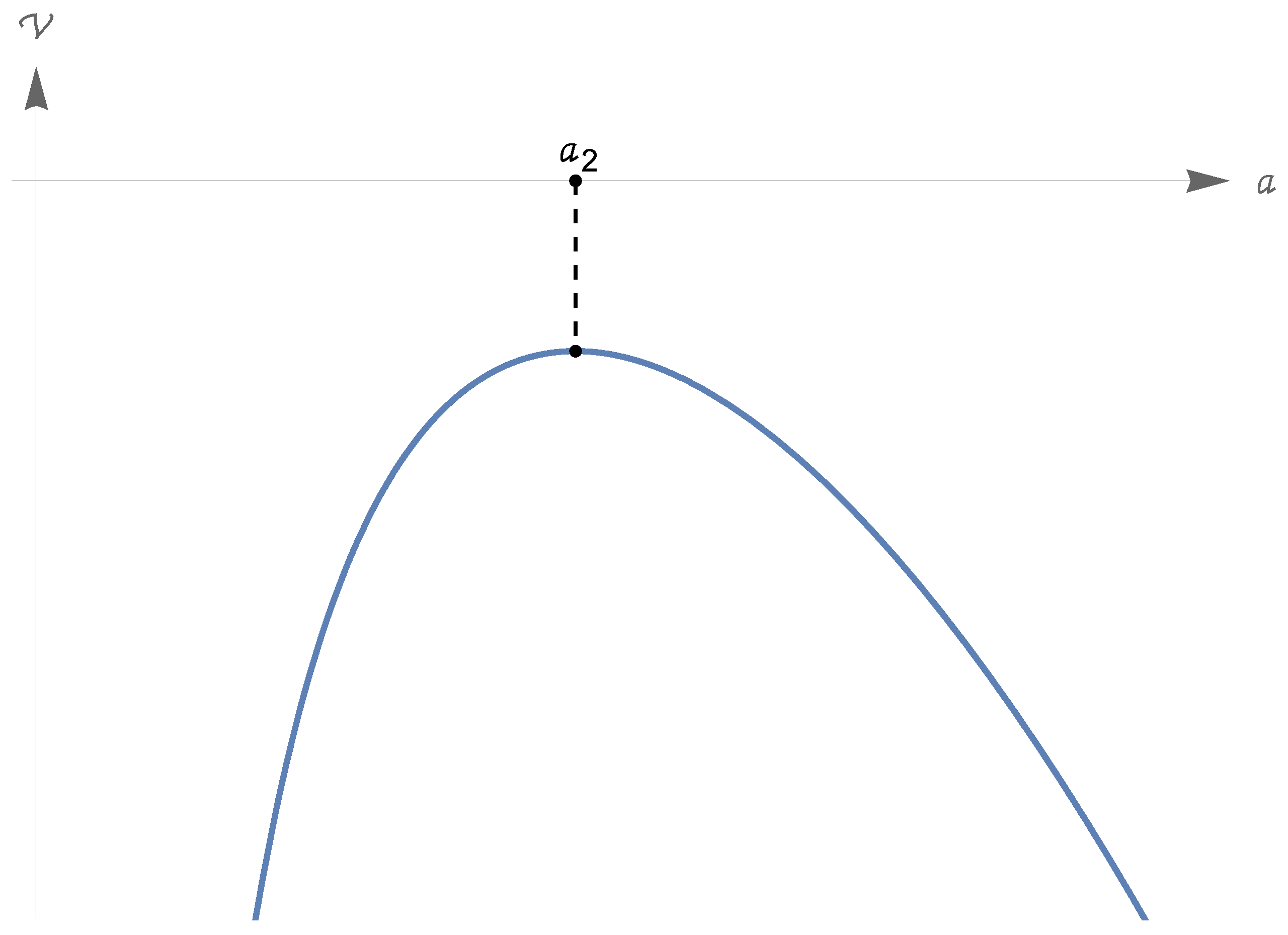
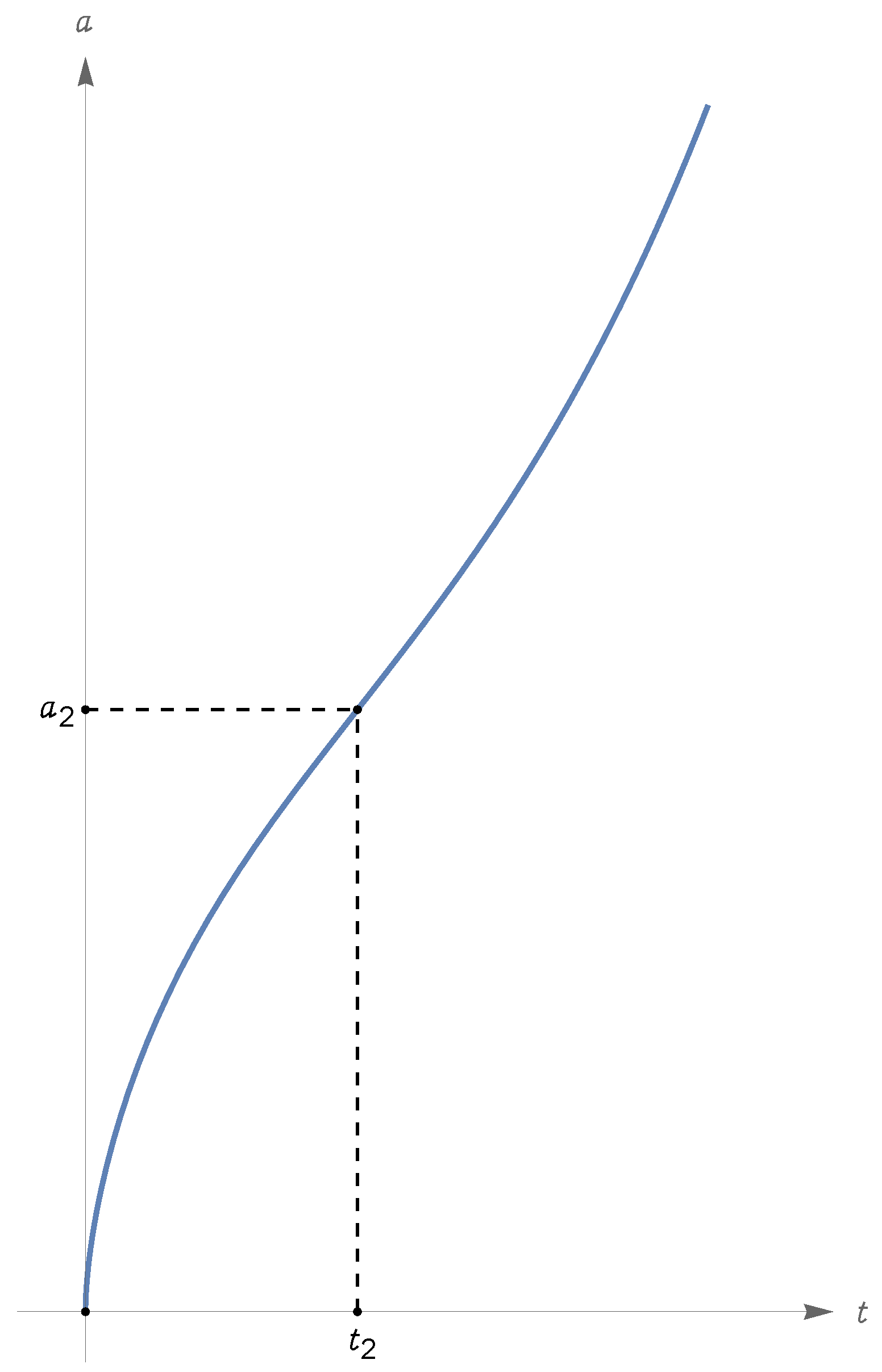
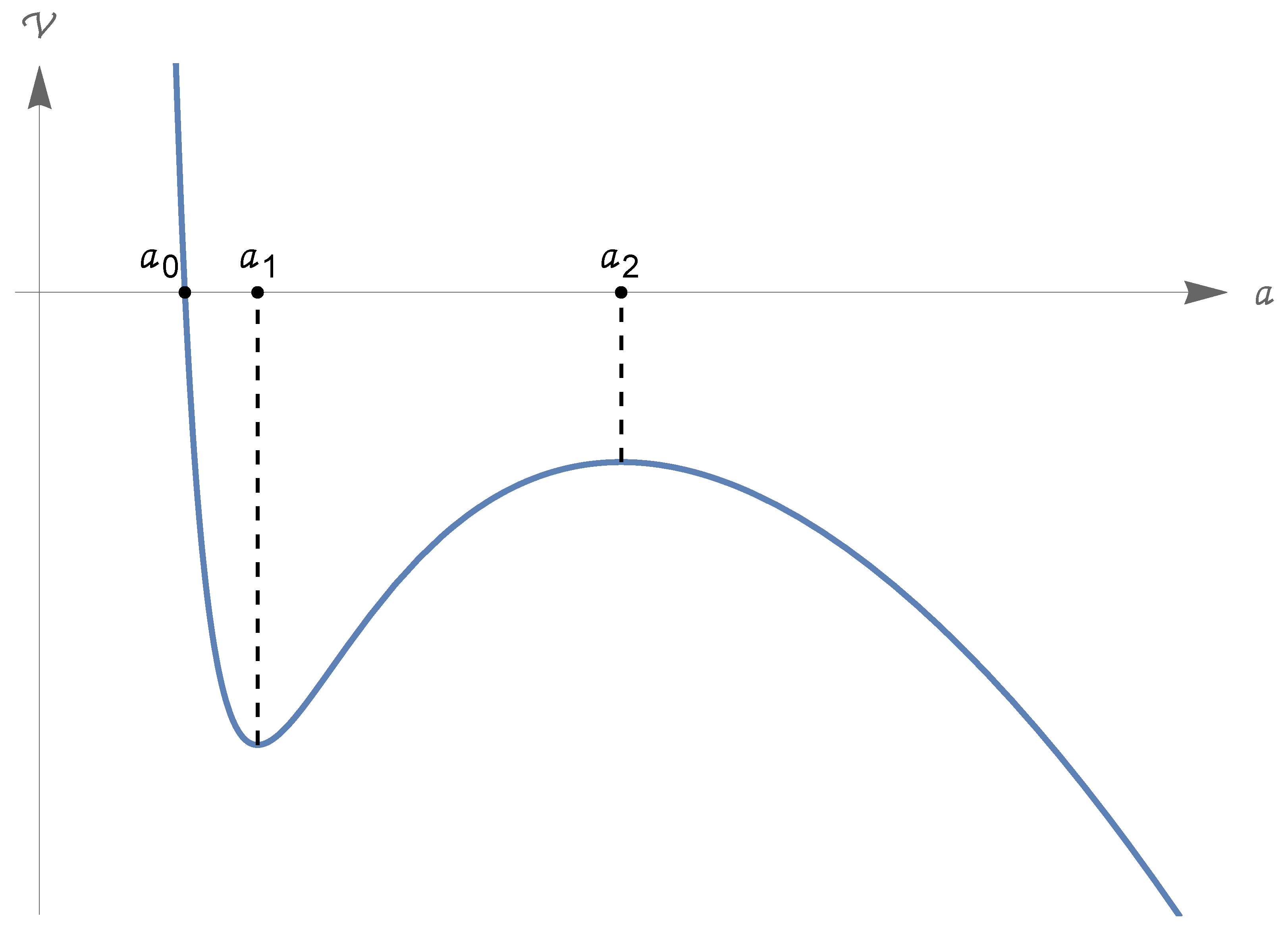
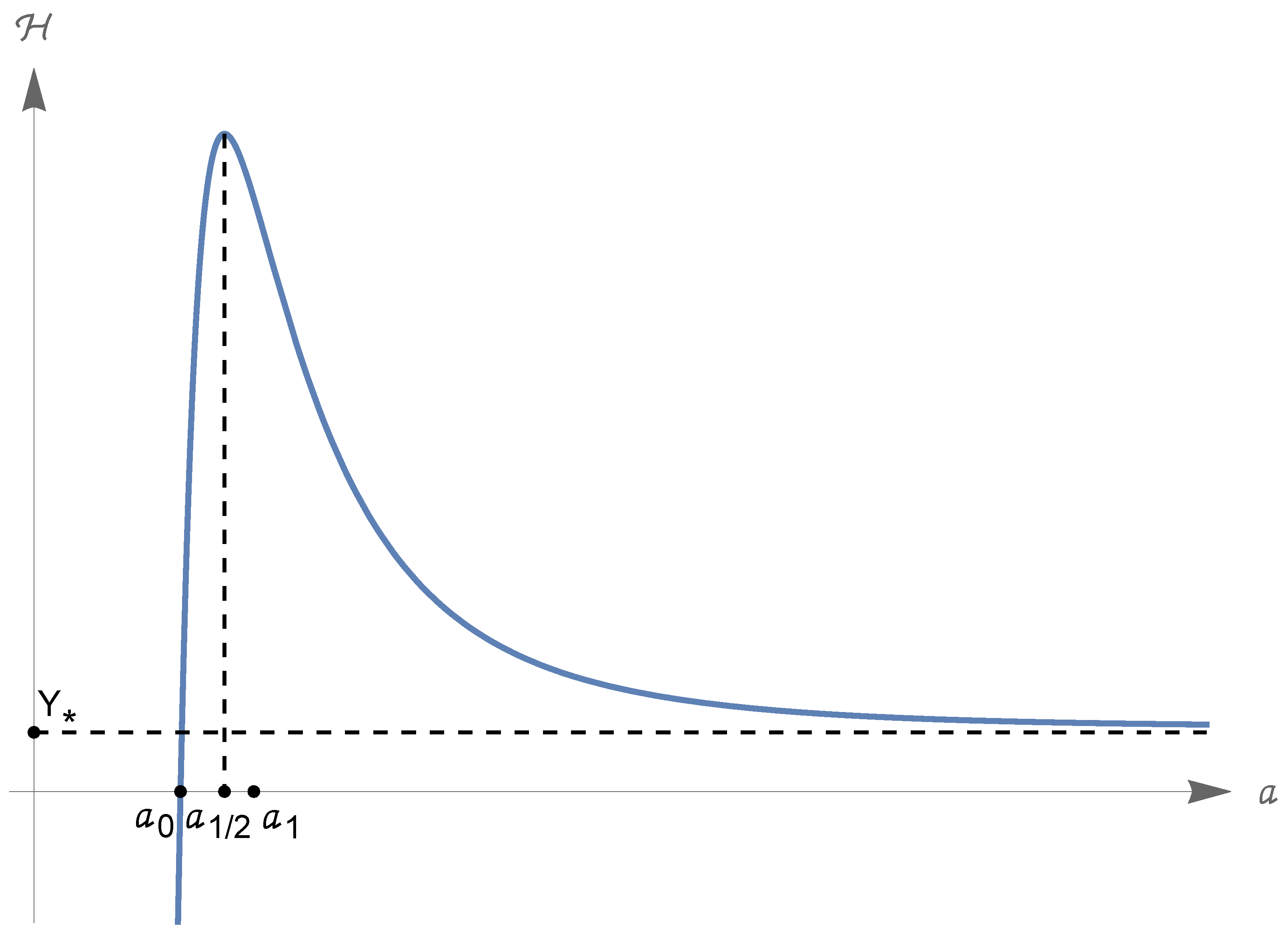
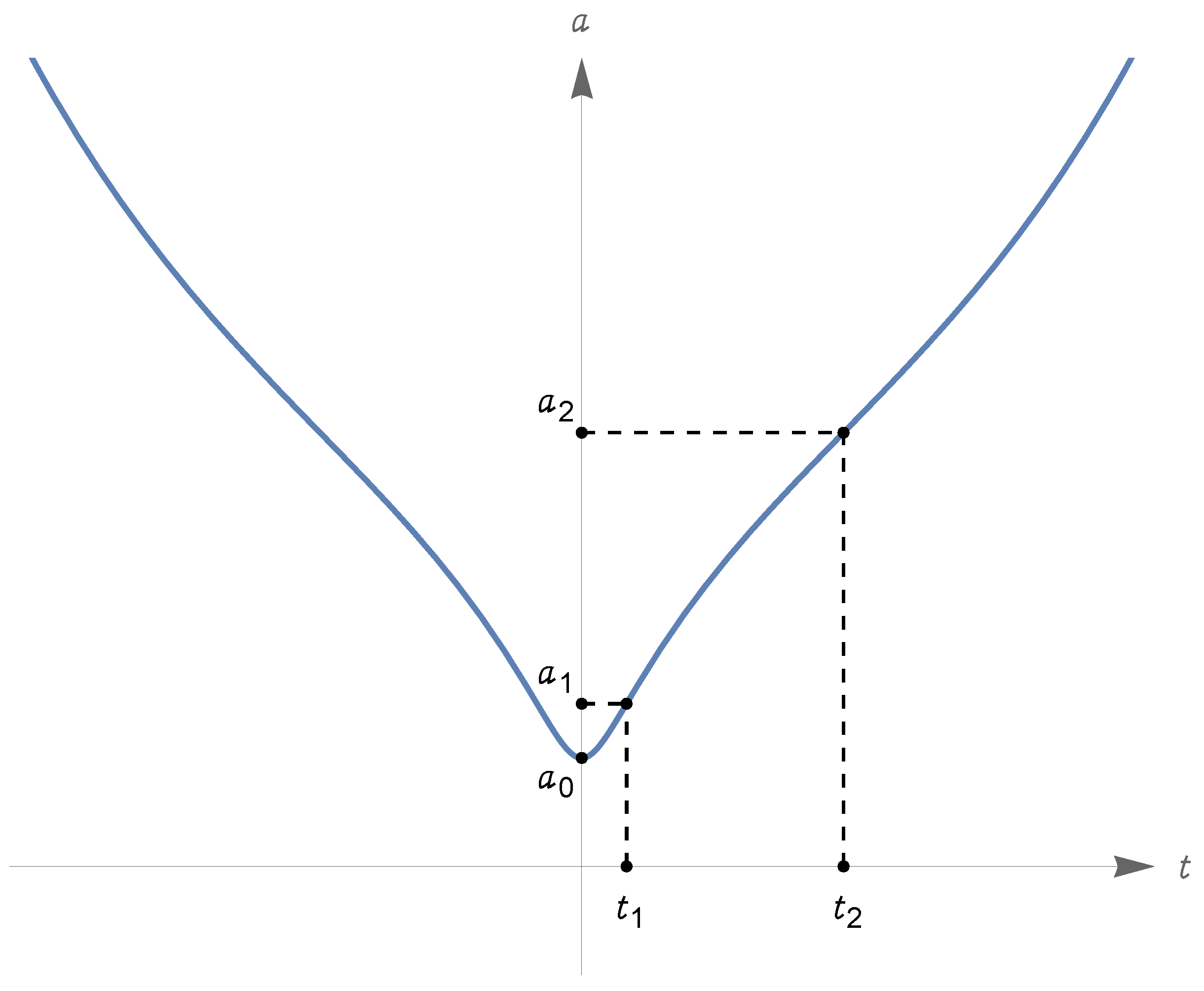
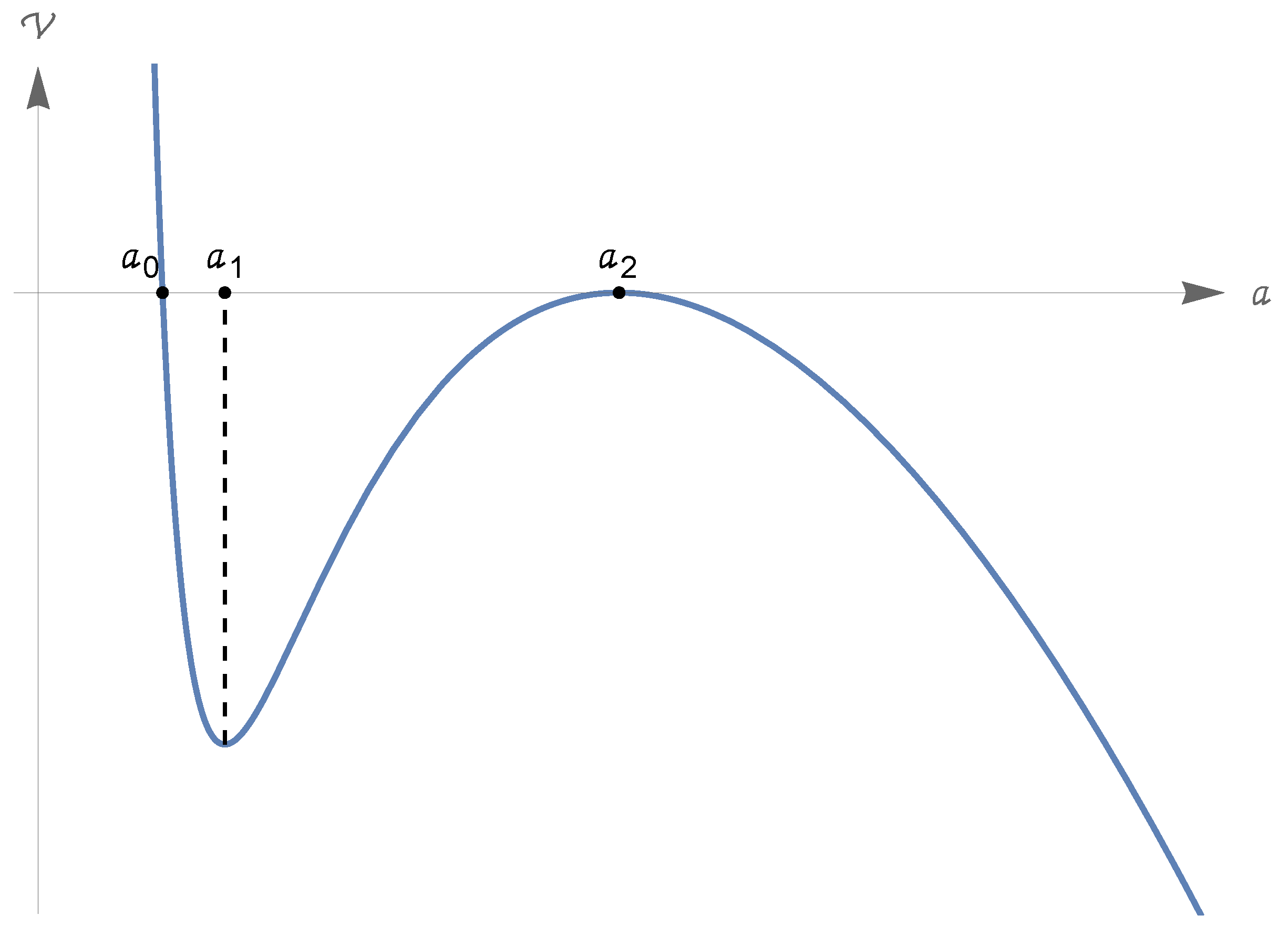
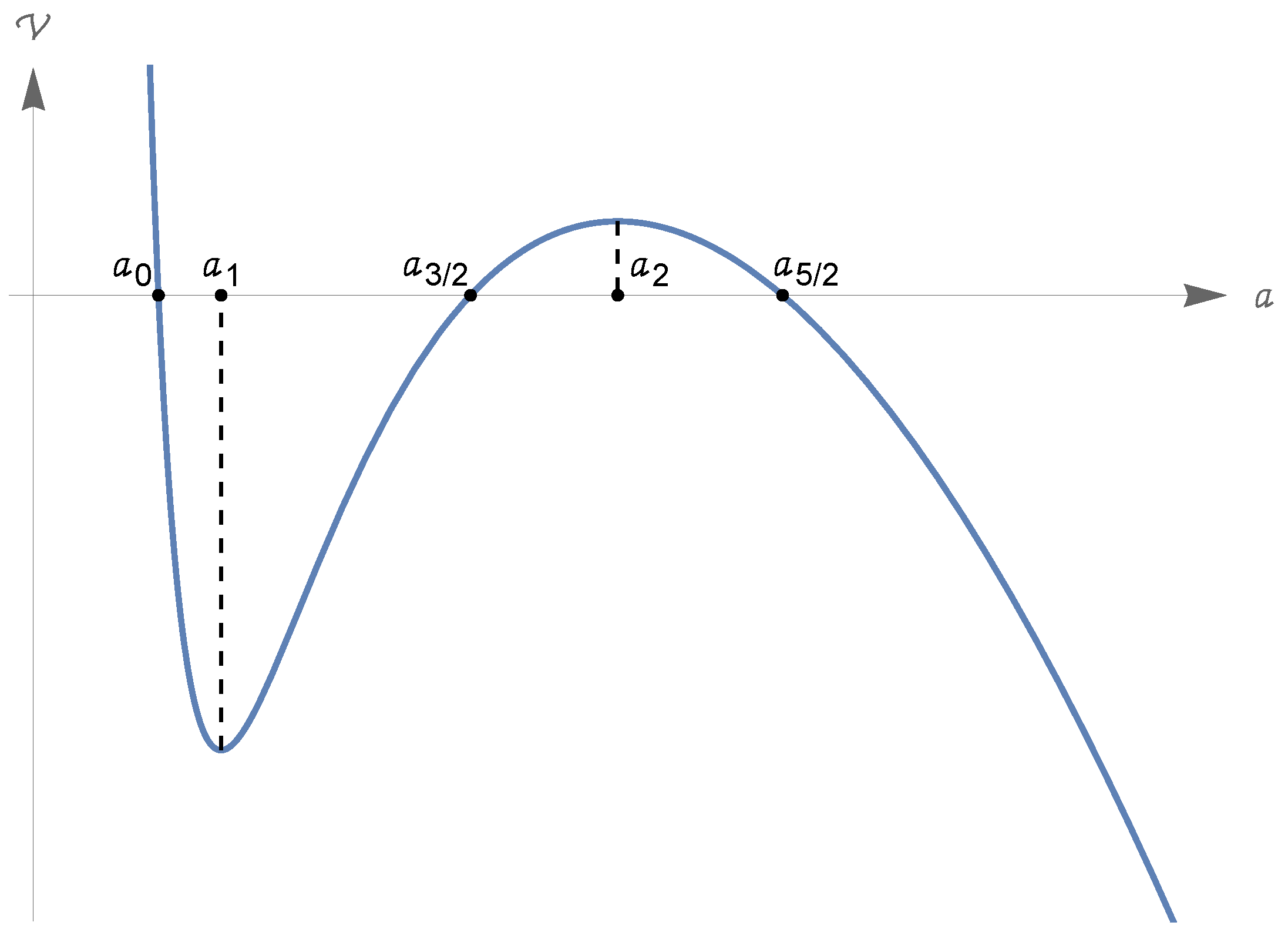
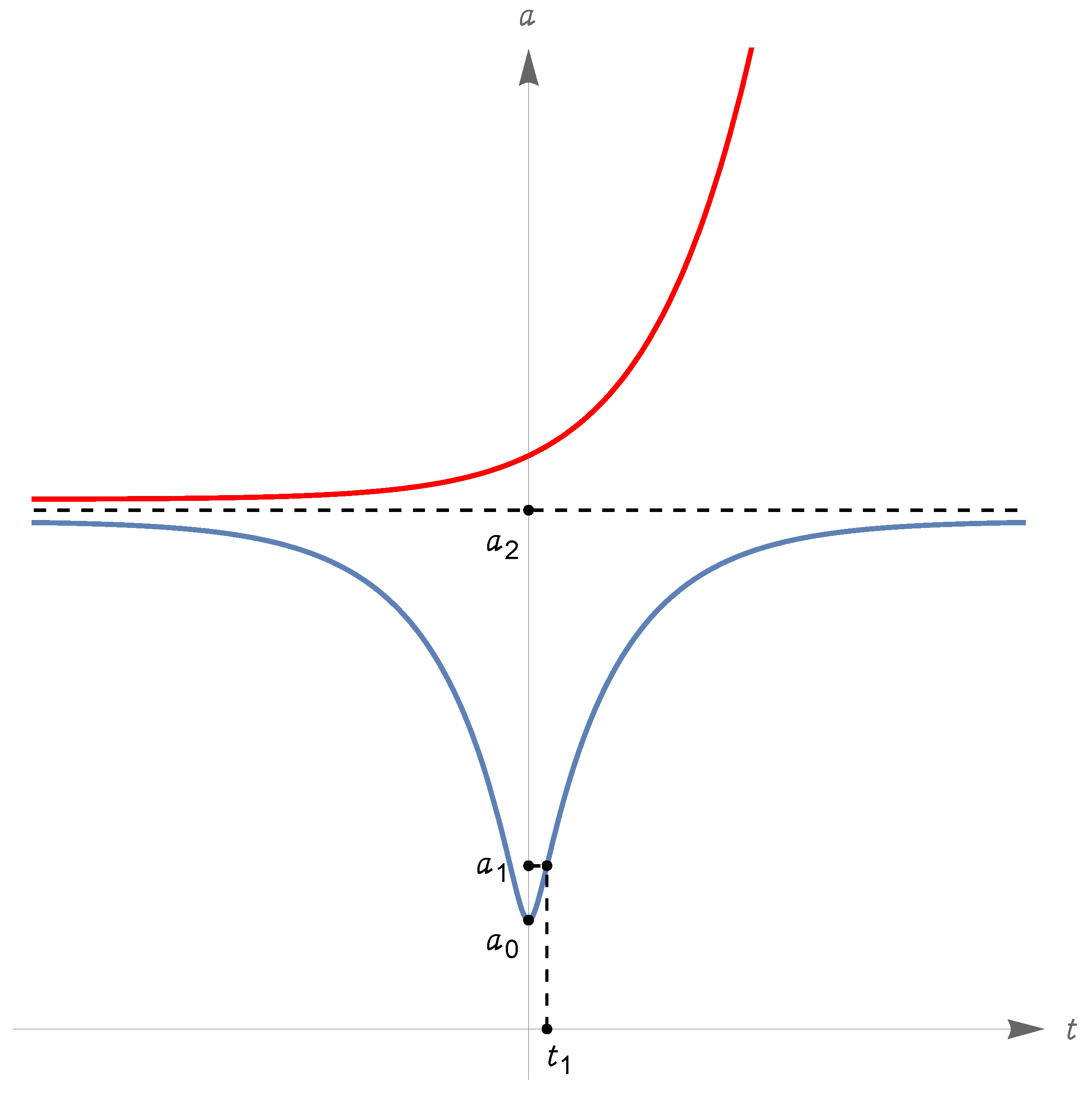
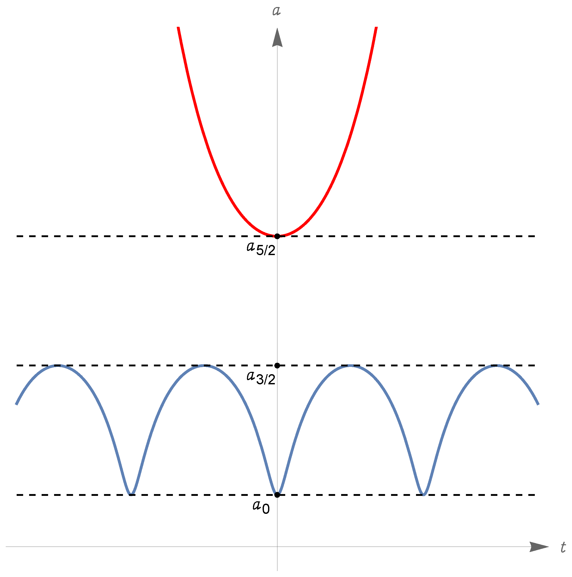
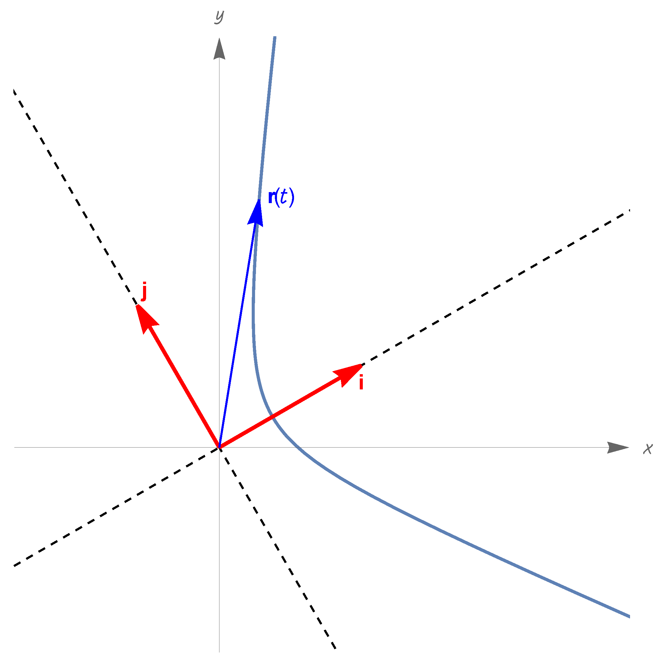
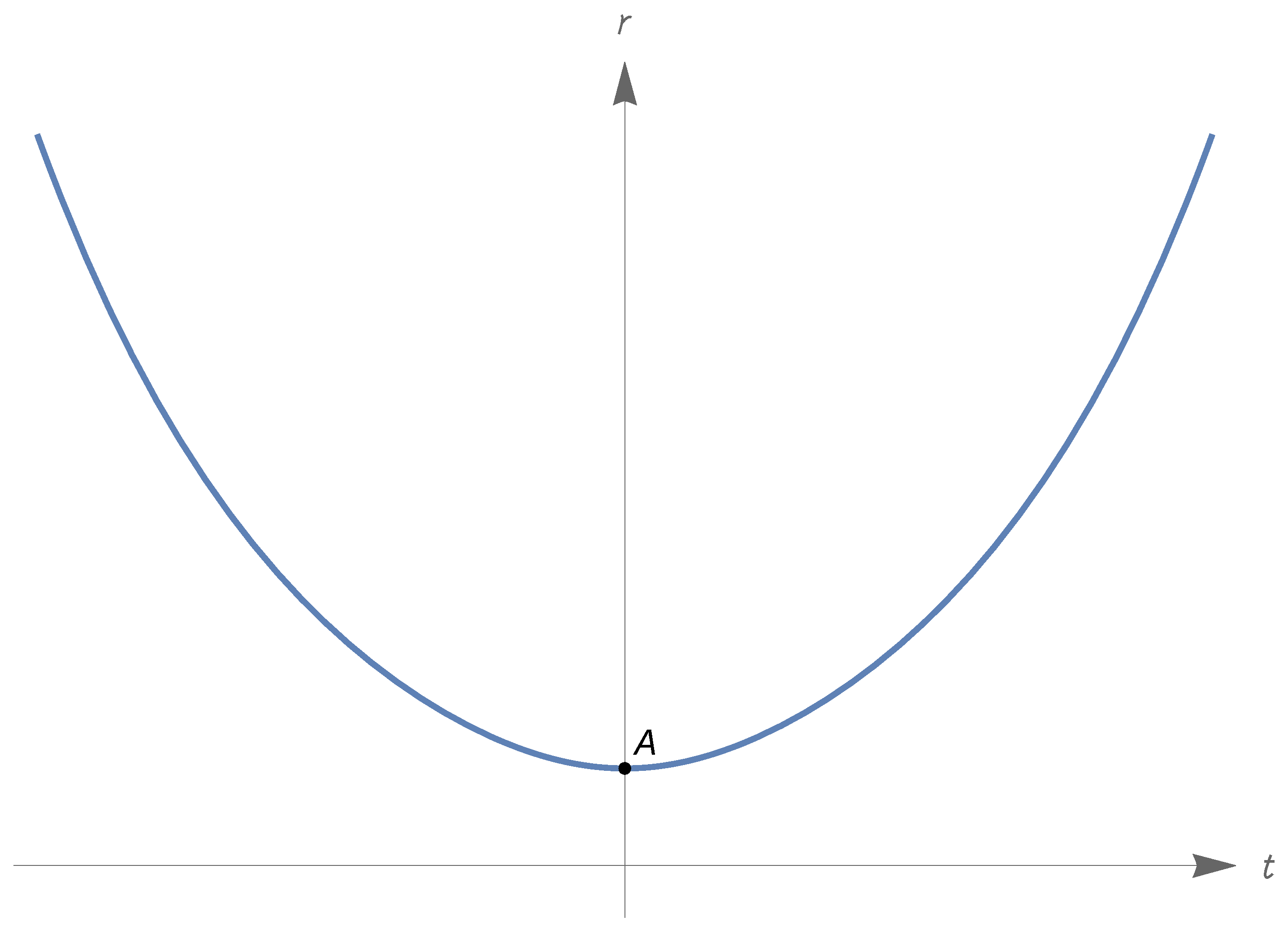
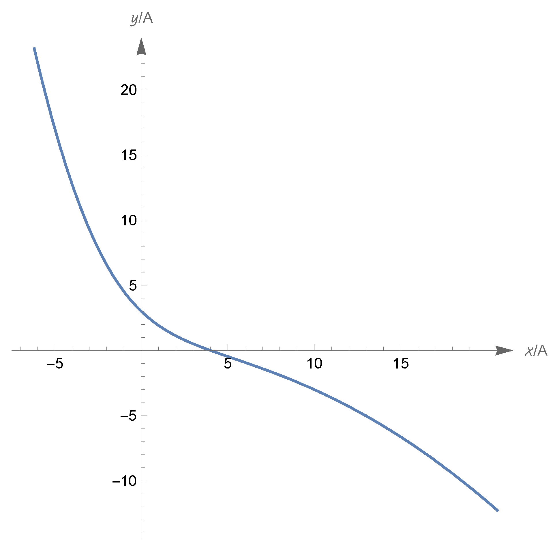
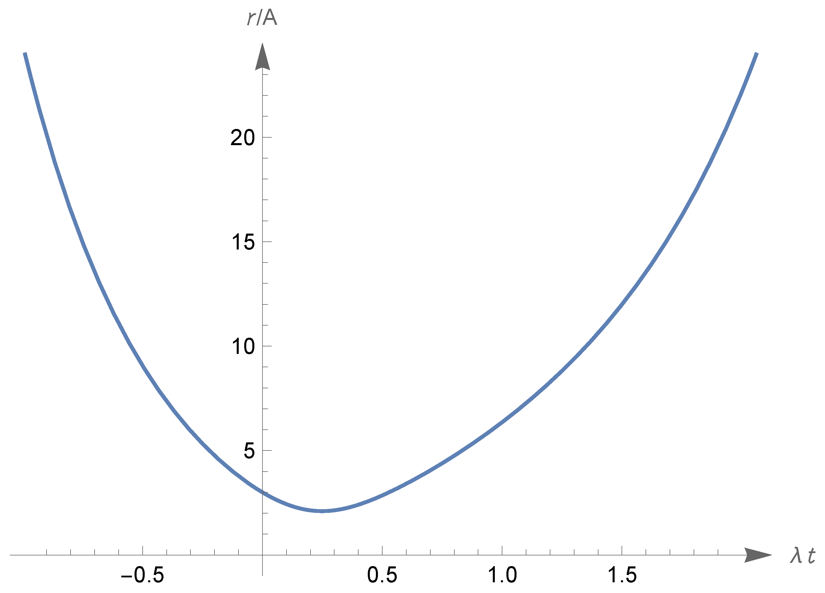
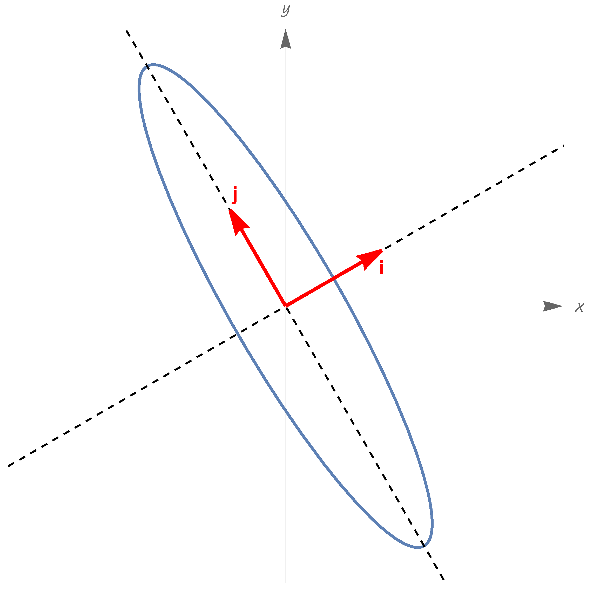

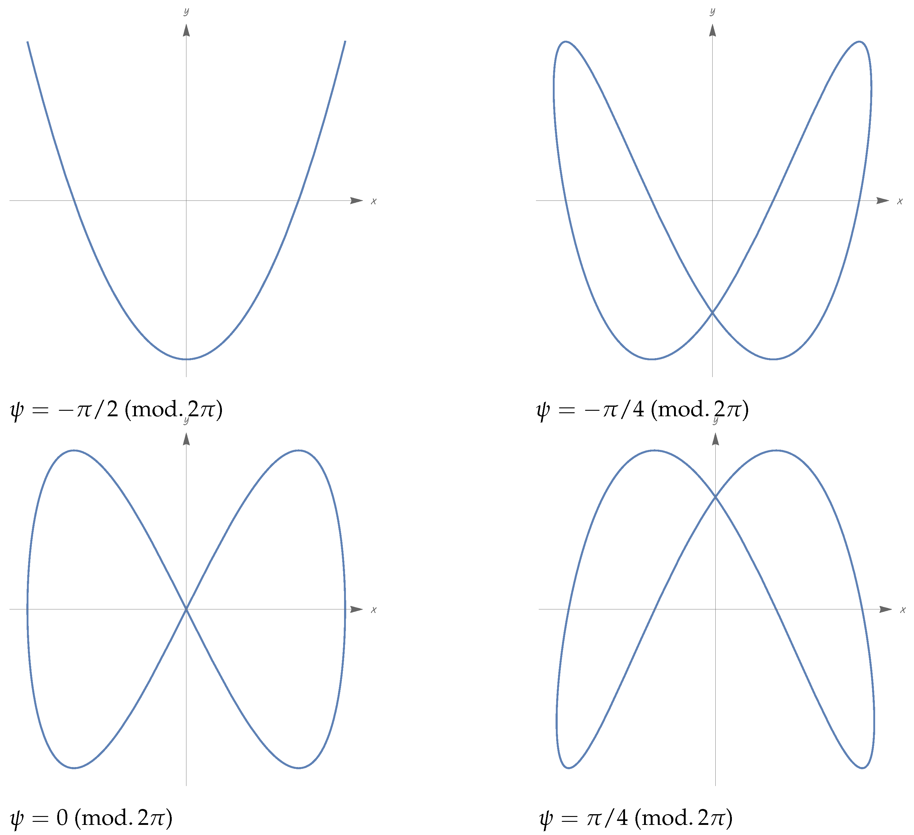
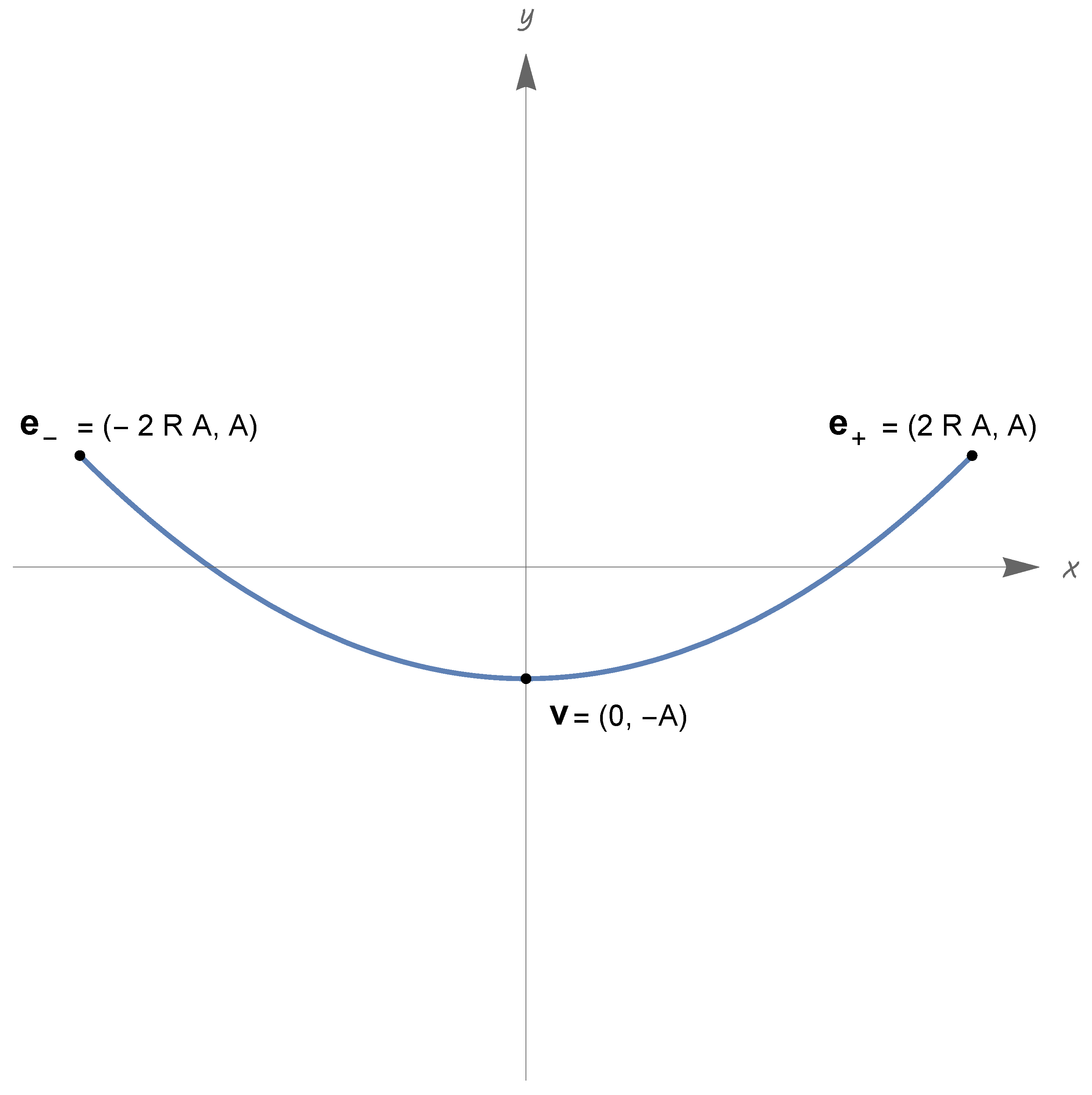
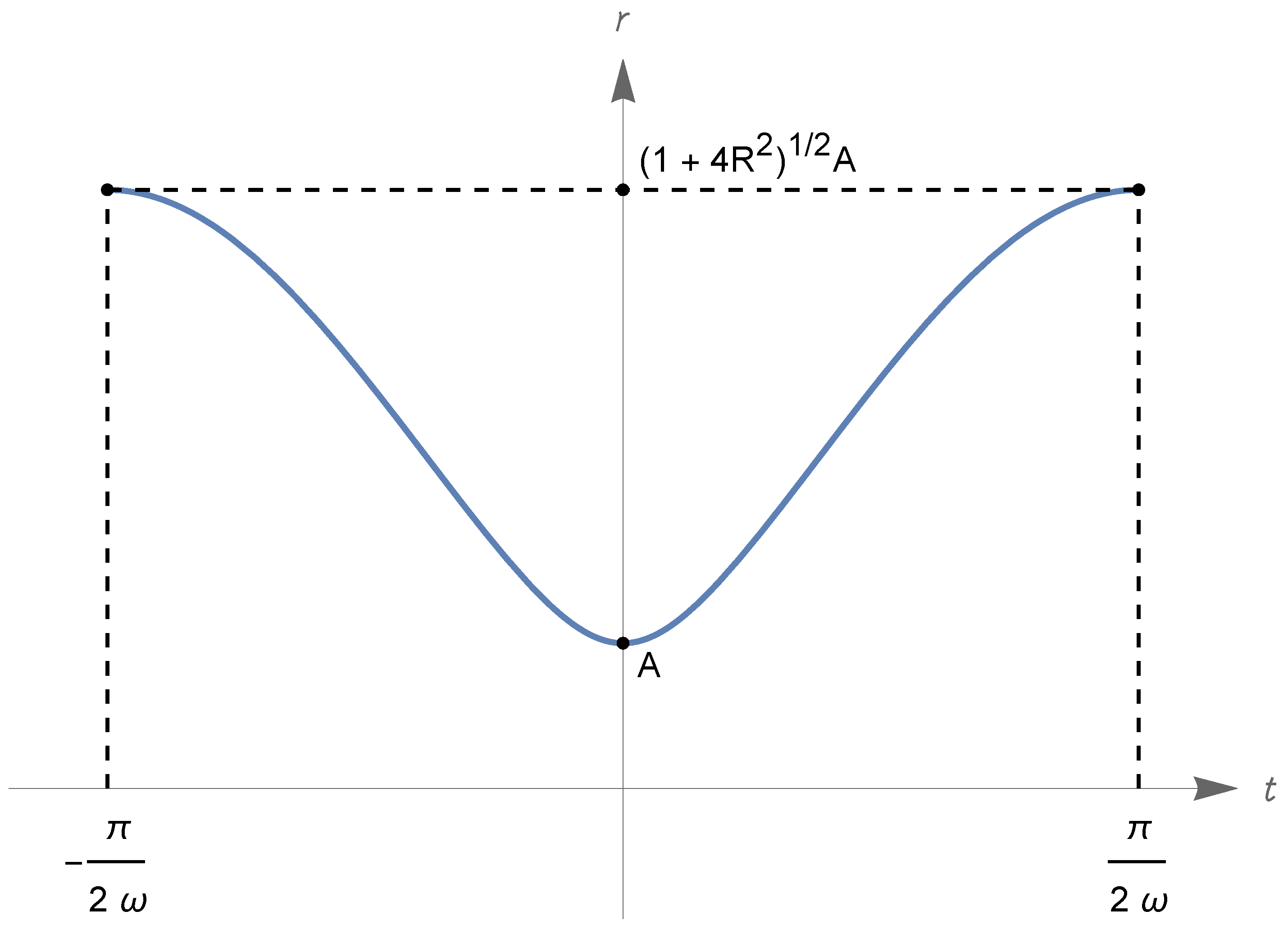
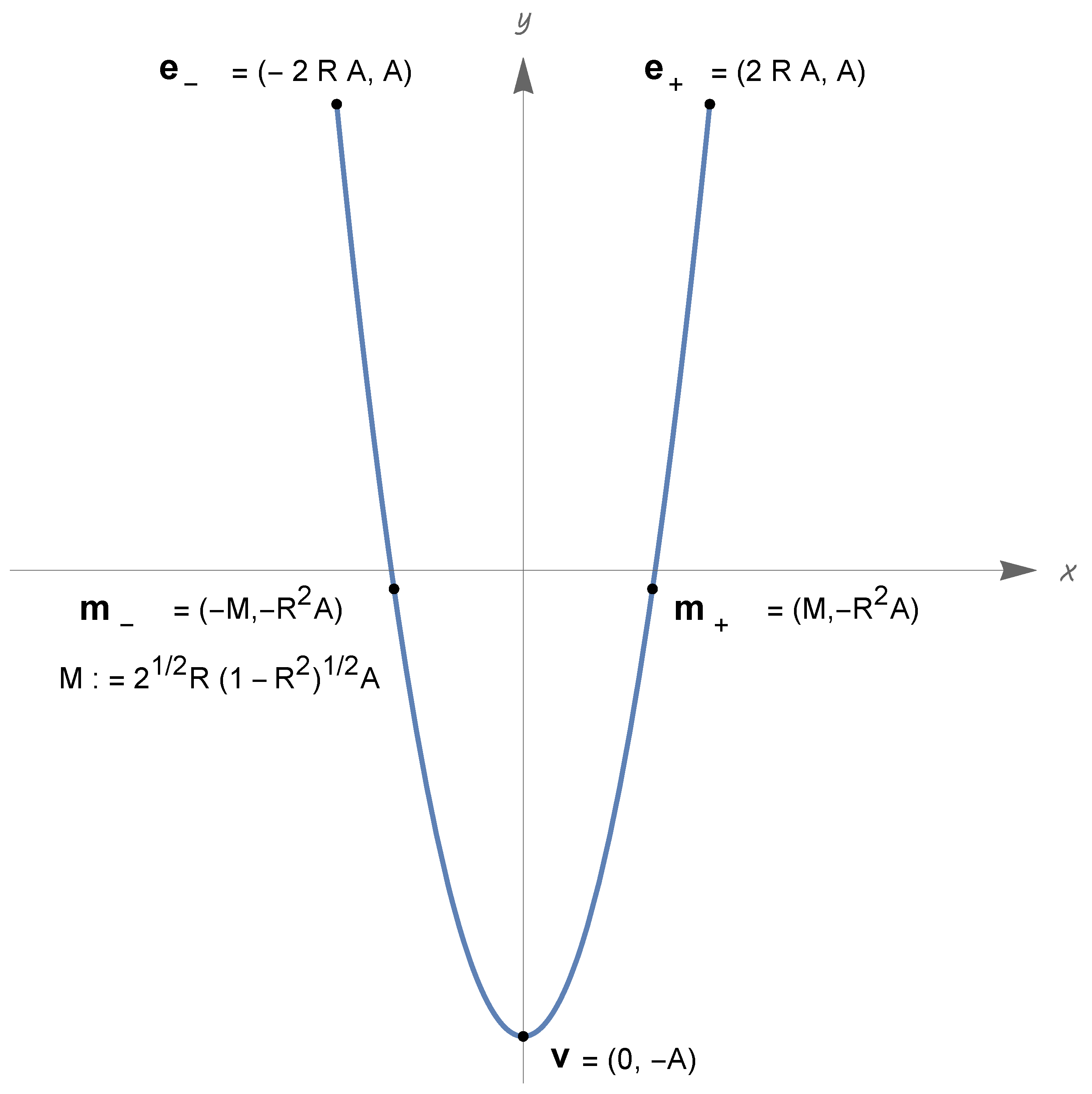

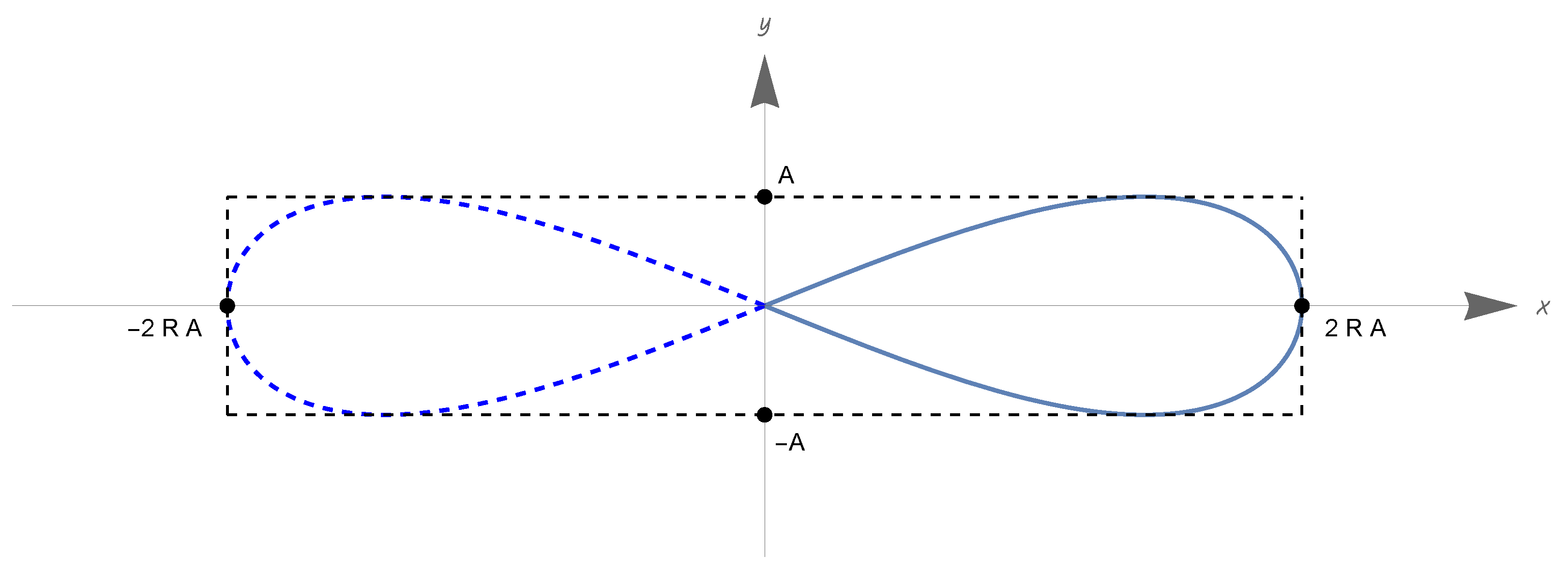
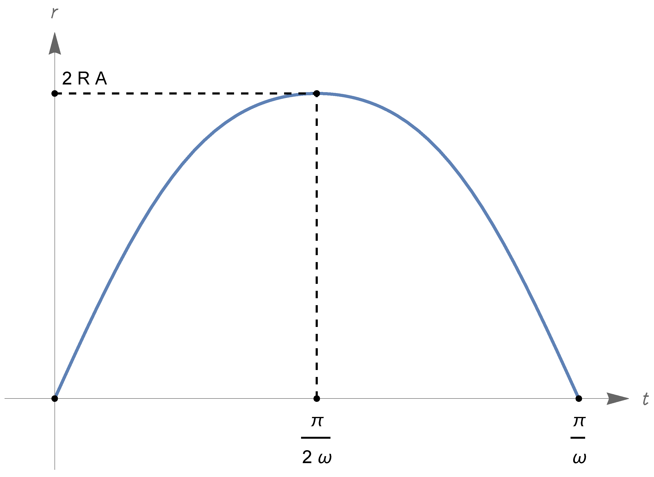
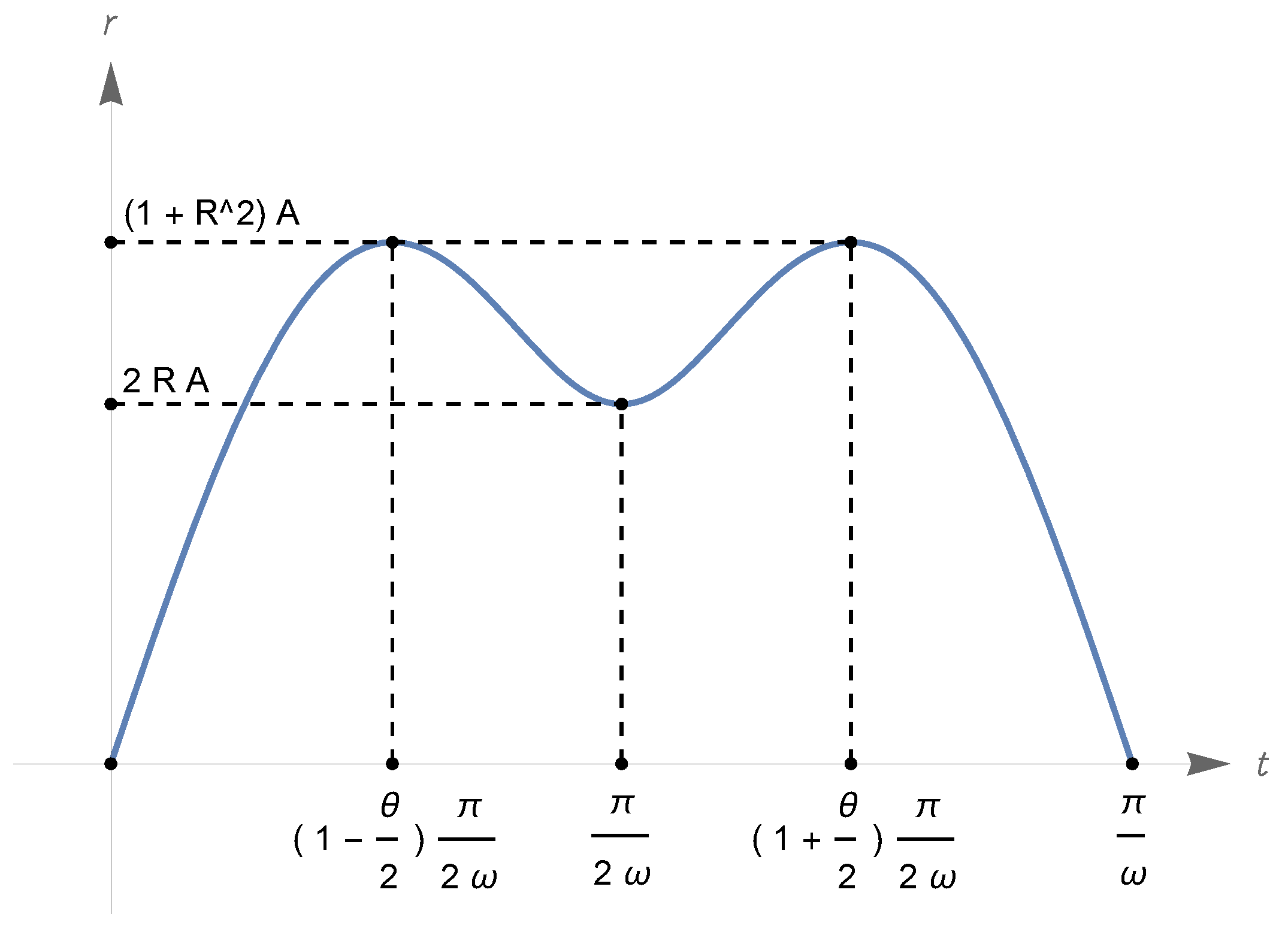
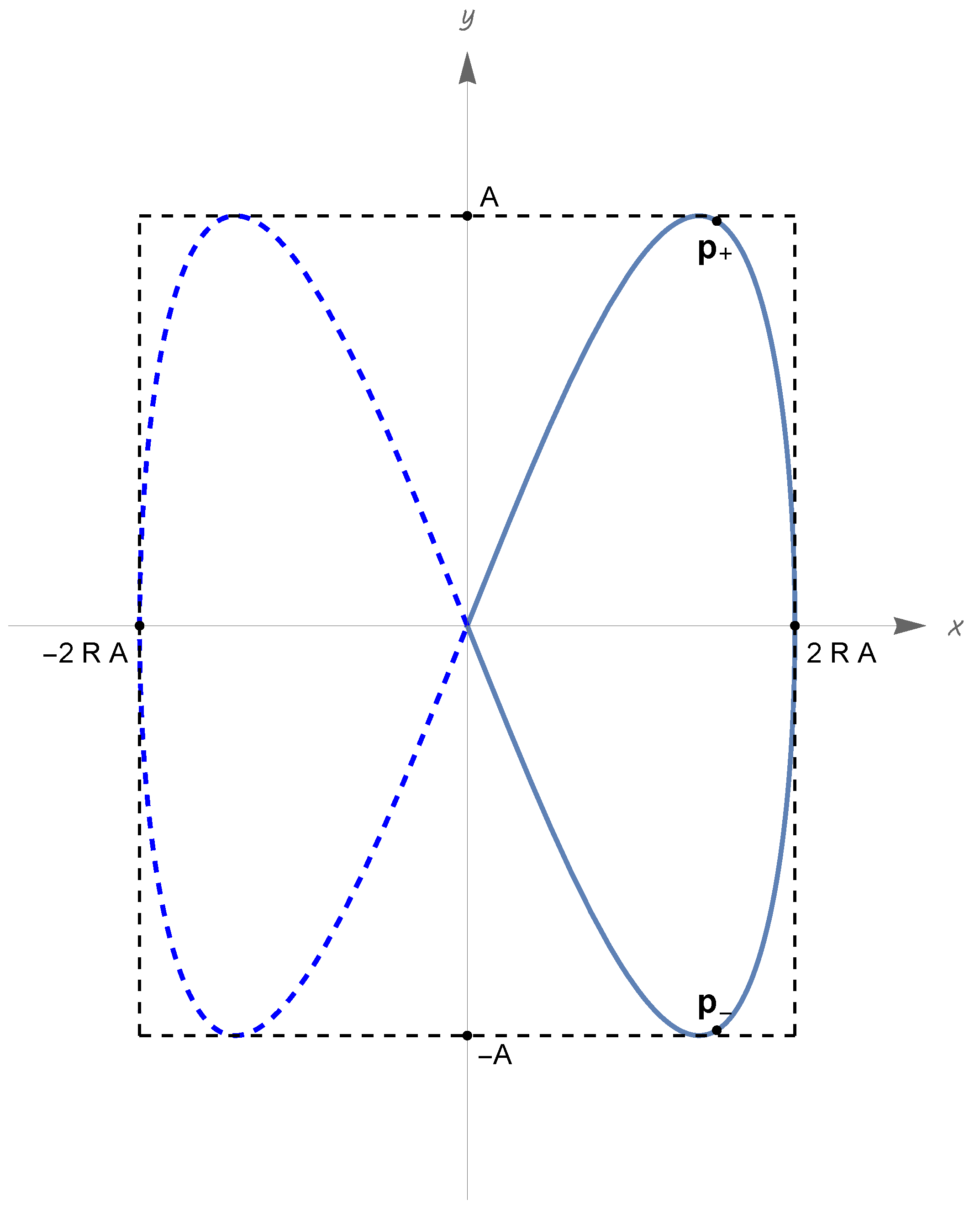
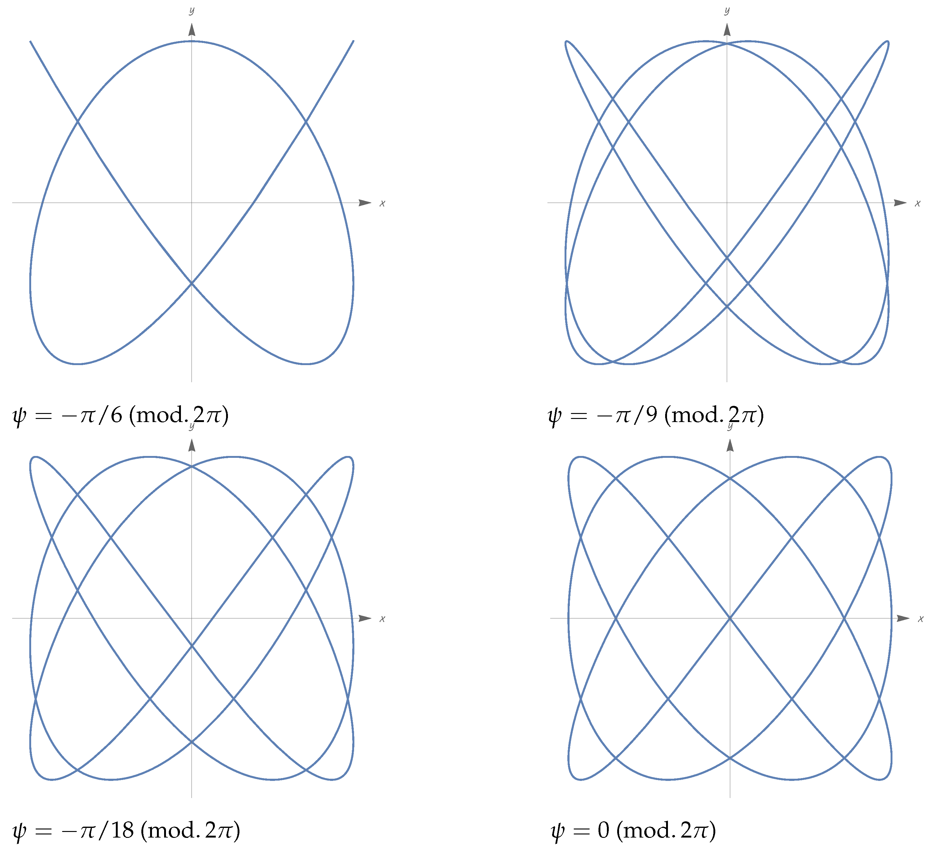
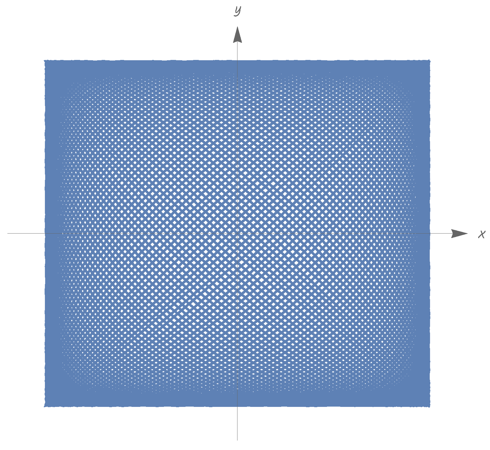
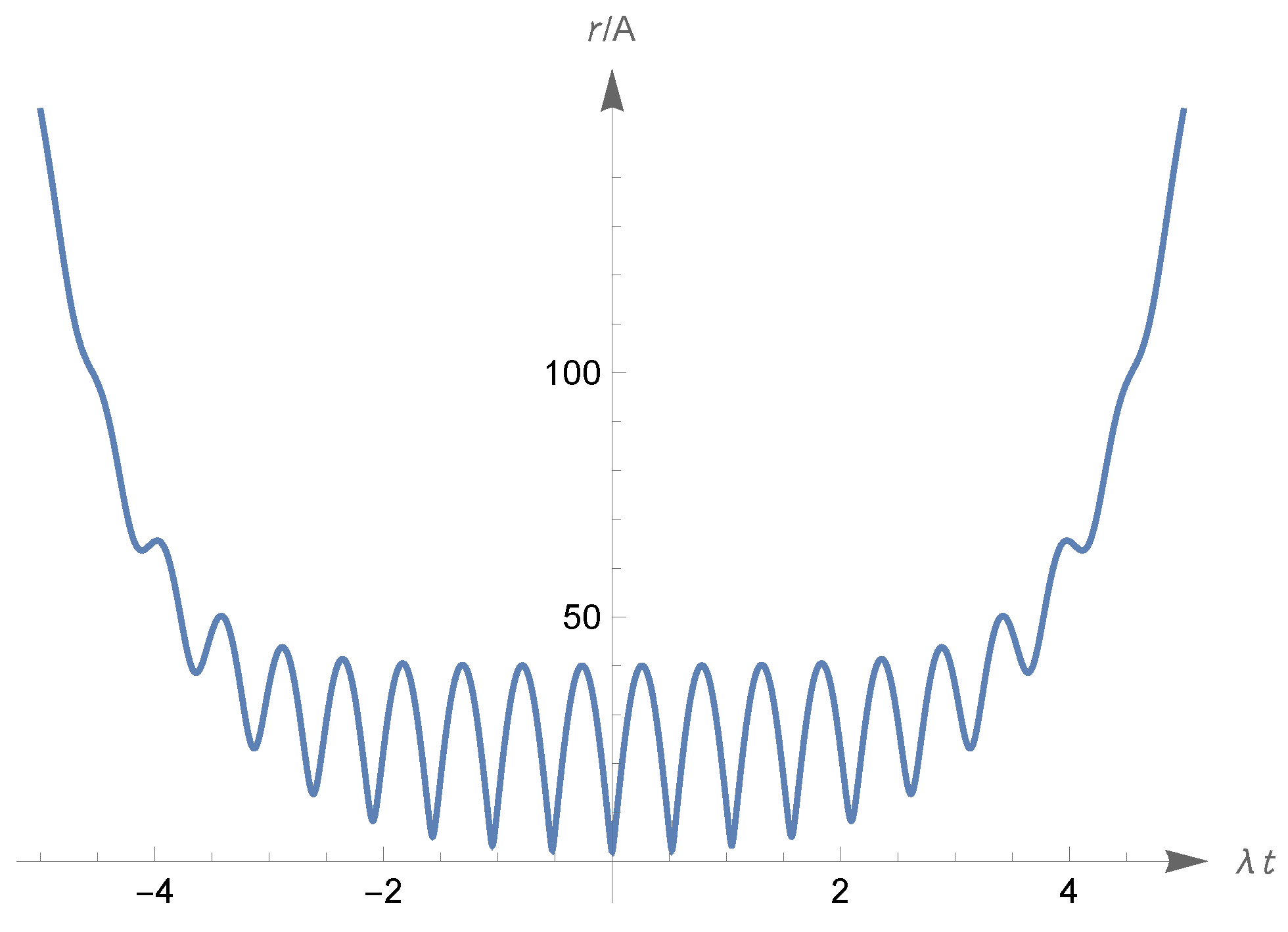
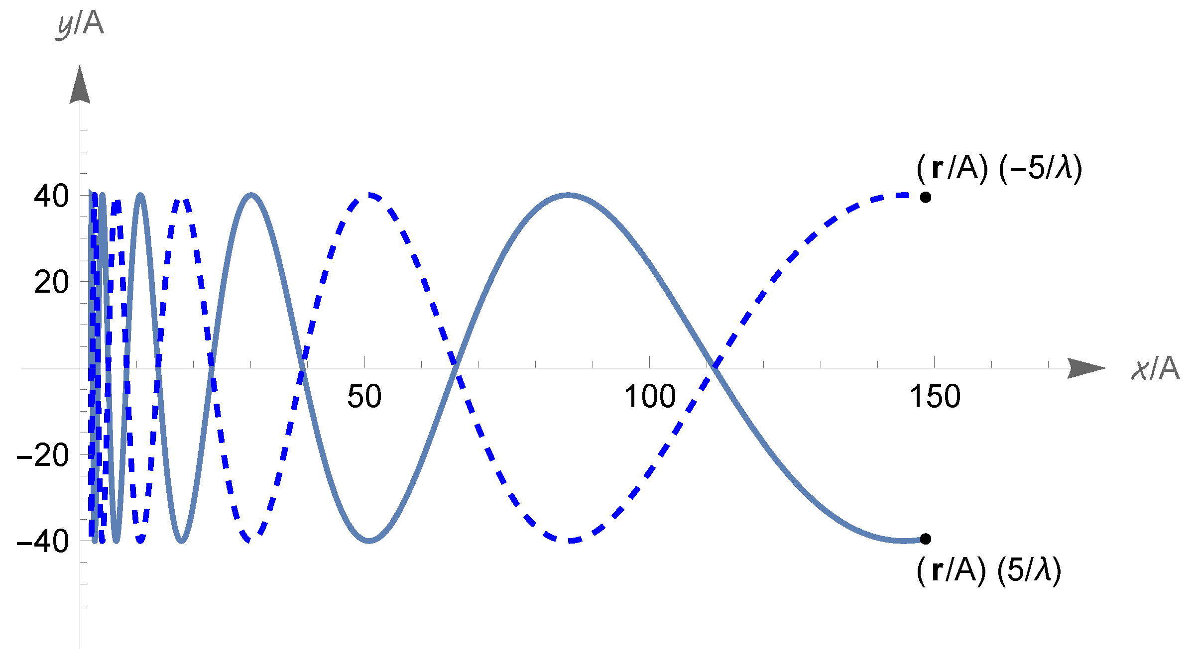
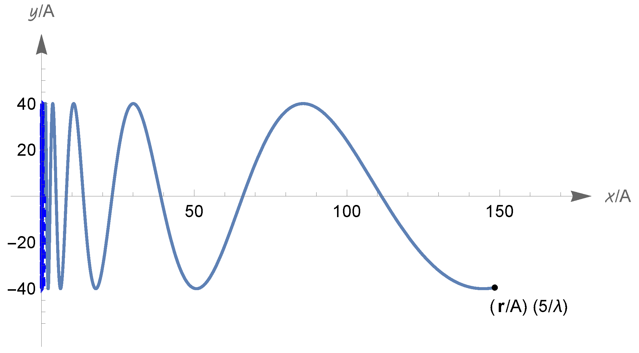
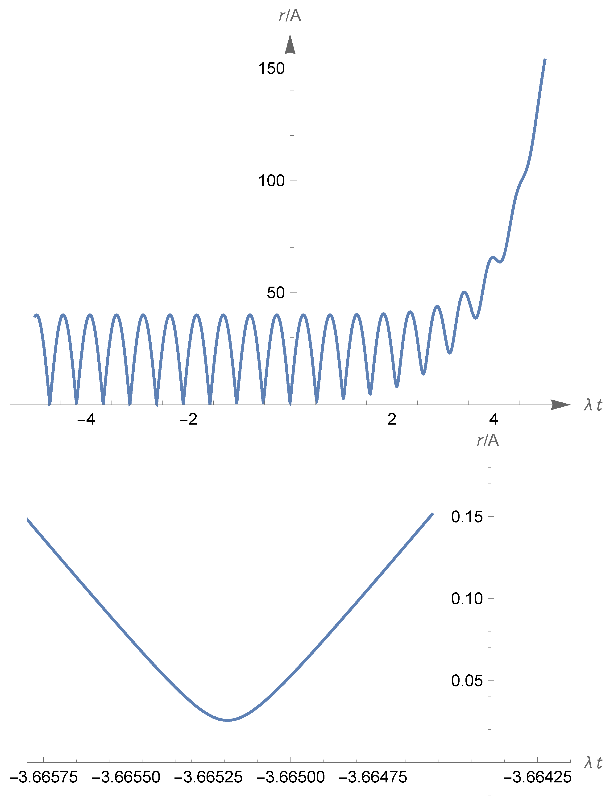
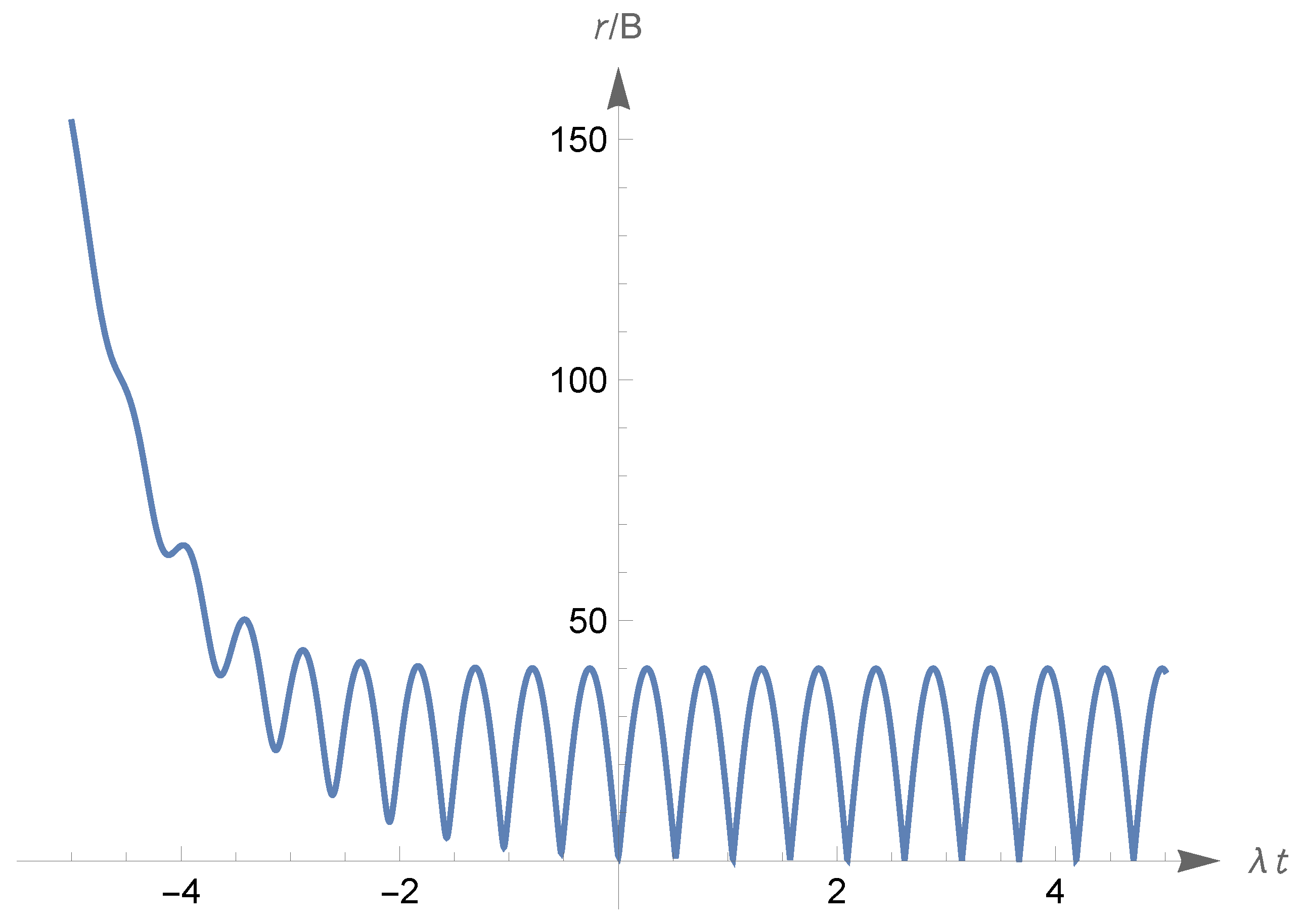
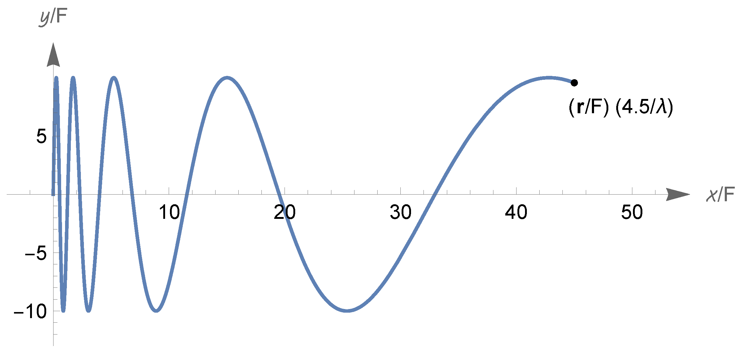
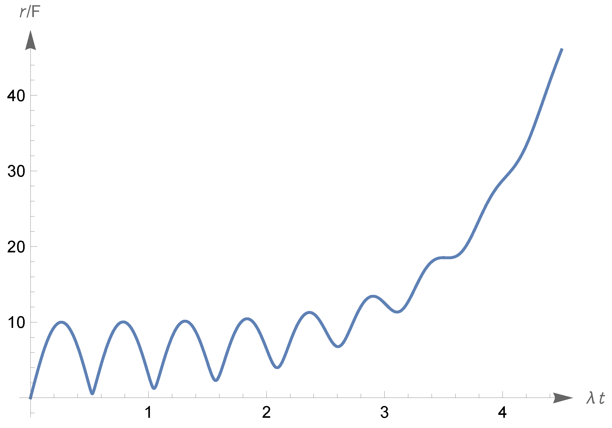
Disclaimer/Publisher’s Note: The statements, opinions and data contained in all publications are solely those of the individual author(s) and contributor(s) and not of MDPI and/or the editor(s). MDPI and/or the editor(s) disclaim responsibility for any injury to people or property resulting from any ideas, methods, instructions or products referred to in the content. |
© 2024 by the authors. Licensee MDPI, Basel, Switzerland. This article is an open access article distributed under the terms and conditions of the Creative Commons Attribution (CC BY) license (https://creativecommons.org/licenses/by/4.0/).