

Cosmologies with Perfect Fluids and Scalar Fields in Einstein’s Gravity: Phantom Scalars and Nonsingular Universes

Abstract
| Contents | ||
| 1. | Introduction | 4 |
| 2. | Generalities on Einstein’s Gravity, Perfect Fluids and Scalar Fields | 11 |
| 2.1. Dimensional Aspects | 11 | |
| 2.2. Conventions About Spacetime, the Einstein Equations, and the Gravitational Constant | 11 | |
| 2.3. Einstein’s Gravity with Perfect Fluids and a Scalar Field | 12 | |
| 3 | FLRW Cosmologies with Perfect Fluids and a Scalar Field | 14 |
| 3.1. Spacetime Structure | 14 | |
| 3.2. Conditions for Timelike or Lightlike Geodesic Completeness: Nonsingular FLRW Spacetimes | 15 | |
| 3.3. Hubble Parameter | 16 | |
| 3.4. The Perfect Fluids | 16 | |
| 3.5. The Scalar Field | 17 | |
| 3.6. The Total Stress–Energy Tensor | 17 | |
| 3.7. Einstein Equations | 17 | |
| 3.8. Klein–Gordon Equation | 18 | |
| 3.9. Conservation Law for the n-th Fluid | 18 | |
| 3.10. Summary of the Evolution Equations | 18 | |
| 3.11. Curvature Density; Normalized Densities | 18 | |
| 3.12. Stationary Points of the Scale Factor | 19 | |
| 3.13. Energy Conditions | 19 | |
| 3.14. The Scale Factor at a Special Time | 20 | |
| 3.15. Dimensionless Formalism | 20 | |
| 4. | Analysis of the Evolution Equations | 24 |
| 4.1. Determining the Fluids’ Densities | 24 | |
| 4.2. The Fluids’ Densities in the Linear Case | 26 | |
| 4.3. The Final Form of the Einstein and Klein–Gordon Equations | 26 | |
| 4.4. Lagrangian Formalism; Zero-Energy Constraint | 27 | |
| 4.5. Again on the Scale Factor at a Special Time | 28 | |
| 4.6. Maximal Solutions | 29 | |
| 5. | The Case with a Constant Potential for the Scalar Field: General Results on the Evolution of and | 29 |
| 5.1. Basic Setting | 29 | |
| 5.2. The Constant of Motion | 30 | |
| 5.3. Reduced Lagrangian | 30 | |
| 5.4. Zero-Energy Solutions of the Reduced System | 31 | |
| 5.5. Time Evolution of the Scalar Field | 32 | |
| 5.6. On Maximal Solutions | 32 | |
| 5.7. Hubble Parameter; Densities and Pressures | 33 | |
| 5.8. The Scale Factor at a Special Time | 33 | |
| 5.9. Comparison with the Literature | 34 | |
| 6. | Again on the Case of = Constant: Big Bounce from a Phantom Scalar | 34 |
| 6.1. Introducing a More Specific Setting | 34 | |
| 6.2. The Case of : Recovering the Standard Model of Cosmology | 36 | |
| 6.3. Introducing the Analysis of Cases with | 40 | |
| 6.4. Preparing the Analysis of the Phantom Case with | 40 | |
| 6.5. The Phantom Case with (Small) and : Analysis of the Potential and the Associated Function | 41 | |
| 6.6. The Phantom Case with (Small) and : Analysis of the Zero-Energy Solutions and Classicality Condition | 45 | |
| 6.7. The Phantom Case with (Small), and Specific Values for All the Parameters | 54 | |
| 6.8. The Phantom Case with (Small) and : Sketching the Basic Results | 57 | |
| 7. | Polar and Cartesian Coordinates for Phantom Cosmologies with a Periodic Field Potential | 62 |
| 7.1. Polar Coordinates (Under Periodicity Assumptions for the Field Potential) | 62 | |
| 7.2. Cartesian Coordinates | 63 | |
| 8. | An Explicitly Solvable Phantom Model with Dust and a Trigonometric Field | 63 |
| 8.1. Some Introductory Considerations | 63 | |
| 8.2. Introducing the Solvable Model | 64 | |
| 8.3. The Case () | 66 | |
| 8.4. Cosmologies with | 66 | |
| 8.5. Cosmologies with and Arbitrary | 69 | |
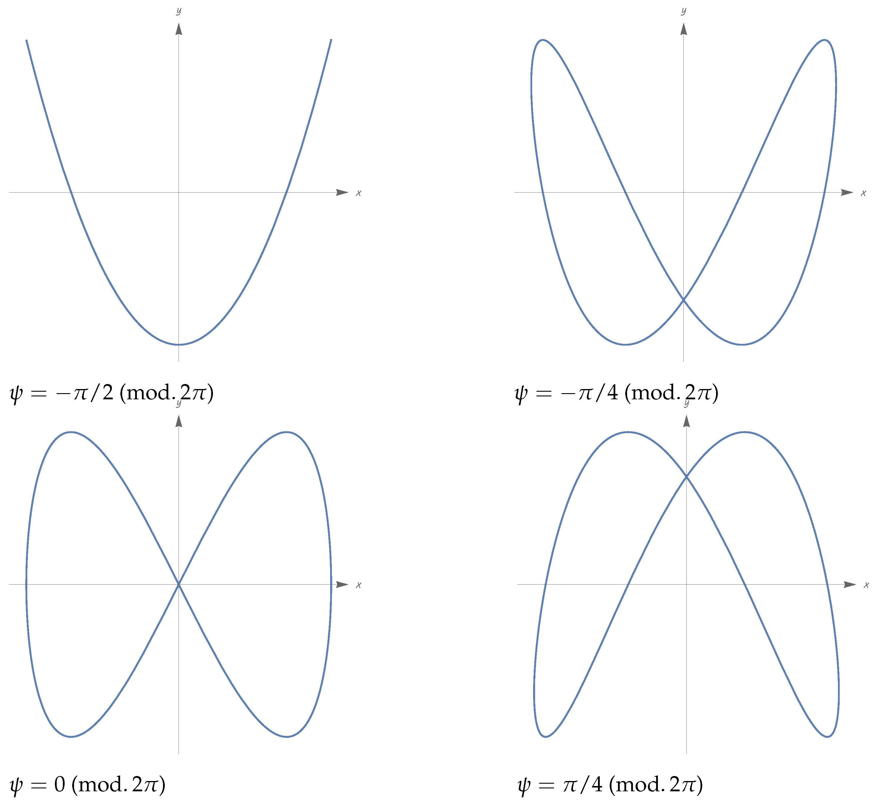
| 8.6. The Case (): Lissajous Cosmologies | 72 | |
| 8.7. Lissajous Cosmologies with | 72 | |
| 8.8. Lissajous Cosmologies with | 75 | |
| 8.9. On General Lissajous Cosmologies | 83 | |
| 8.10. The Case | 86 | |
| 8.11. Again on the Case , | 88 | |
| 9. | Concluding Remarks | 93 |
| Appendix A. | Riemannian Manifolds, Spacetimes, and Dimensional Analysis | 93 |
| Appendix B. | FLRW Spacetimes and Generalizations | 94 |
| Appendix C. | Time Orientation of a Spacetime: The Case of a Generalized FLRW Spacetime | 95 |
| Appendix D. | A Review on Geodesics and Several Associated Notions of Completeness, Mainly in Riemannian Manifolds and in Spacetimes. Nonsingular Spacetimes | 96 |
| Appendix E. | Geodesics and Geodesic Completeness of Generalized FLRW Spacetimes | 98 |
| Appendix F. | A Review the Energy Conditions | 106 |
| Appendix G. | On the Determination of the Fluids’ Densities | 106 |
| Appendix H. | Comparing the Zero Energy Motions of Two One-Dimensional Lagrangians | 107 |
| Appendix I. | The Descartes’ Rule of Signs | 107 |
| Appendix J. | Two Statements on a Class of Polynomials | 108 |
| Appendix K. | Proof of Statements (185) and (186) on the Potential of the Standard Cosmological Model | 110 |
| Appendix L. | Proof of Statements (a)–(d) in Section 6.5 about the Function of Equation (201) | 111 |
| Appendix M. | Proof of Statements (f)–(i) in Section 6.5 about the Function of Equation (220) | 114 |
| Appendix N. | Proof of Equation (250) (Including Convergence of an Integral Therein) | 116 |
| Appendix O. | Proof of Some Statements about in Equation (271) | 117 |
| Appendix P. | A Usefulf Inequality | 118 |
| Appendix Q. | Estimates on the Time in Equation (244) | 119 |
| Appendix R. | Further Estimates on the Time in Equation (244) | 122 |
| Appendix S. | On the Quantity in Equation (292) | 125 |
| Appendix T. | A More Detailed Description of the Model in Section 6.7 | 128 |
| Appendix U. | Proof of Statements (-) in Section 6.8 about the Function of Equation (201) | 128 |
| Appendix V. | Derivation of Equations (363)–(366) | 130 |
| Appendix W. | Derivation of Equations (401) and (402) | 132 |
| Notes | 132 | |
| References | 136 | |
1. Introduction
- (i)
- To review the general setting for FLRW cosmologies with non-interacting perfect fluids and with a (canonical or phantom) scalar field, possibly self-interacting and minimally coupled to gravity, with special attention to the Lagrangian formalism.
- (ii’-ii”)
- To explore some exactly solvable cases of the previous setting for FLRW cosmologies, which have received (to our knowledge) little or no attention in the literature; these special cases often involve phantom scalar fields and yield nonsingular cosmological models.
- (ii’)
- To discuss the case where the self-potential of the scalar field is constant, paying special attention to a subcase with pressureless matter, radiation, and a phantom scalar, yielding a Big Bounce cosmology.
- (ii”)
- To propose a solvable FLRW cosmological model with a phantom scalar, a specific self-interaction potential of trigonometric type and pressureless matter. This model is treated passing from the coordinates to suitably defined “Cartesian” coordinates ; when the coefficients of the self-interaction potential are negative, the trajectories of the model in the space are Lissajous curves.
2. Generalities on Einstein’s Gravity, Perfect Fluids and Scalar Fields
2.1. Dimensional Aspects
2.2. Conventions About Spacetime, the Einstein Equations, and the Gravitational Constant
2.3. Einstein’s Gravity with Perfect Fluids and a Scalar Field
- N species of non-interacting perfect fluids, all of them with the same - velocity. For any , we suppose that the n-th fluid has a positive mass–energy density and a pressure . We have and where is the space of mass densities mentioned in Section 2.1, which coincides with the space of pressures in our setting with . We assume a barotropic equation of state of the following form:The above-mentioned perfect fluids can include, for example, dust () and a radiation gas ().3
- A classical scalar field , minimally coupled to gravity and self-interacting with potential . We have , where is an appropriate real, one-dimensional, oriented vector space. For dimensional reasons that will soon be clarified, we require and . No direct interaction is assumed between the scalar field and the above-mentioned perfect fluids.
3. FLRW Cosmologies with Perfect Fluids and a Scalar Field
3.1. Spacetime Structure
3.2. Conditions for Timelike or Lightlike Geodesic Completeness: Nonsingular FLRW Spacetimes
- Past timelike complete, or past lightlike complete, or past complete if each maximal, future-directed geodesic of the timelike, lightlike , or of both types is past complete;
- Future timelike complete, or future lightlike complete, or future complete if each maximal, future-directed geodesic of the timelike, lightlike , or of both types is future complete;
- Timelike complete, lightlike complete or complete if it possesses the above-defined properties both in the past and future (meaning that the maximal geodesics of the types mentioned above are defined on the full interval ).
- Past timelike complete, if and only if
- Past lightlike complete, if and only if(without requiring );
- Future timelike complete, if and only if
- Future lightlike complete, if and only if(without requiring ).
3.3. Hubble Parameter
3.4. The Perfect Fluids
3.5. The Scalar Field
3.6. The Total Stress–Energy Tensor
3.7. Einstein Equations
3.8. Klein–Gordon Equation
3.9. Conservation Law for the n-th Fluid
3.10. Summary of the Evolution Equations
3.11. Curvature Density; Normalized Densities
3.12. Stationary Points of the Scale Factor
3.13. Energy Conditions
3.14. The Scale Factor at a Special Time
3.15. Dimensionless Formalism
- Past timelike complete, if and only if
- Past lightlike complete, if and only if(without requiring );
- Future timelike complete, if and only if
- Future lightlike complete, if and only if(without requiring ).
4. Analysis of the Evolution Equations
4.1. Determining the Fluids’ Densities
- (i)
- It isIn this case, for each , the function of (101) is defined implicitly by the following quadrature formula:(This formula actually individuates a unique smooth function ; see again Appendix G).
- (ii)
- It is
4.2. The Fluids’ Densities in the Linear Case
4.3. The Final Form of the Einstein and Klein–Gordon Equations
4.4. Lagrangian Formalism; Zero-Energy Constraint
- (i)
- The Einstein equation and the Klein–Gordon equation are equivalent to the Lagrange equations induced by L.
- (ii)
- The Einstein equation is equivalent to the zero-energy constraint ; along solutions of the Lagrange equations, this constraint is fulfilled at all times if and only if it is fulfilled at a particular time .
4.5. Again on the Scale Factor at a Special Time
- (i)
- There is a zero-energy solution of the Lagrange equations induced by L, such that , at some time .
- (ii)
- There are such that
4.6. Maximal Solutions
5. The Case with a Constant Potential for the Scalar Field: General Results on the Evolution of and
5.1. Basic Setting
5.2. The Constant of Motion
5.3. Reduced Lagrangian
5.4. Zero-Energy Solutions of the Reduced System
- (i)
- For all t in the (open, real) interval , one has . So, the image of the function is an interval contained in the following set:Of course, this is the union of the subsetswhich must be distinguished for a qualitative analysis of the solution.
- (ii)
- The equations and have well known implications. In particular, if is an instant, one has if and only if ; if, in addition, , then is an inversion time, i.e., is nonzero with different signs when t ranges in two suitable intervals and (this is readily inferred from the relations and ).
- (iii)
- If is an interval such that = constant for all , everywhere in this interval, we haveso that, by separation of variables,(If or is an endpoint of , in the above formula, or should be intended as the limit of for or ).
- (iv)
- The considerations in (iii) bring to our attention integrals of the following form:let us assume, e.g., and for all . If and , the integral (149) is certainly convergent. Convergence is also ensured if vanishes but is nonvanishing, at one or both endpoints . For example, let and ; then, by Taylor’s formula, for , we have , so that the integrand in (149) diverges in an integrable way near .
- (v)
- If is such that , , the constant function for all is a zero-energy solution (indicated in the sequel as an equilibrium solution).
- (vi)
- A nonconstant, zero-energy solution requires an infinite time to reach a point such that , . To explain this statement, let us consider, e.g., the case of a zero-energy solution such that at some time and assume, with , that and for . If the solution is maximal (i.e., if its time domain cannot be furtherly extended; see Section 4.6), for , it will exist, with , until reaching point . According to item (iii), will be reached at the time such thaton the other hand, the above integral diverges, i.e.,In fact, the assumptions , and Taylor’s formula grant the existence of such that for ; this implies , which ensures divergence of the integral in (150).The above argument has obvious variants. For example, again with and , let us consider a maximal zero-energy solution such that at some time and assume, with , that and for . Then, exists for until reaching in the past of ; this occurs at time .
- (vii)
- Under specific assumptions, one can also discuss the time required for a maximal solution to diverge to . In this discussion, one essentially uses Equation (148), sending to one of the extremes of integration; an example of these considerations will appear in Section 6.6, in the lines before Equation (241).
- (viii)
- Due to Equation (143) , we haveso, the concavity and the inflexion points in the graph of a solution can be determined by studying the sign of along the solution.
5.5. Time Evolution of the Scalar Field
- (i)
- Due to (136), for all , we havethe function is constant if , and strictly monotonic if .
- (ii)
- Consider an interval on which has constants sign , as in item (iii) of Section 5.4. Then, the function is a diffeomorphism between and the interval where and . We now consider the inverse function , and the composition . Recalling Equations (136) and (147), we findso that, integrating between and ,(as in the comment after Equation (148), here, or must be intended as a limit if or is an endpoint of ; the same can be said of or ).
5.6. On Maximal Solutions
5.7. Hubble Parameter; Densities and Pressures
5.8. The Scale Factor at a Special Time
- (i)
- There is a zero-energy solution of the Lagrange equations induced by L such that the canonically conjugate momentum of the scalar field has the assigned value , and , at some time .
- (i’)
- There is a zero-energy solution of the Lagrange equations induced by , with the assigned value , such that , at some time .
- (ii)
- It is
5.9. Comparison with the Literature
6. Again on the Case of = Constant: Big Bounce from a Phantom Scalar
6.1. Introducing a More Specific Setting
- (a)
- For the spatial dimension, we assume the realistic valuelet us recall Equation (4), involving the usual gravitational constant G.
- (b)
- There are fluids, referred to as radiation and matter and indicated with the labels r and m, respectively; consequently, all formulas of the previous sections will be rephrased assuming the values for the fluids’ index n. Radiation is described in the standard way and matter is supposed to behave like dust, so the corresponding equations of state are as follows:
- The spatial curvature has the general representation (71).
- Equation (158) for the normalized energy densities reads, in this case,with the dimensionless Hubble parameter.
- According to Equation (132), the present setting with a field potential const. can be rephrased in terms of the Einstein equations with a cosmological constant
- (c)
- It is(positive field potential or positive cosmological constant).
- (d)
- The values considered for the constants (), and are in any case related as follows:
6.2. The Case of : Recovering the Standard Model of Cosmology
6.3. Introducing the Analysis of Cases with
- (i)
- (phantom scalar field), (typically small), (i.e., );
- (ii)
- (phantom scalar field), (typically small), (i.e., );
- (iii)
- (canonical scalar field), ;
6.4. Preparing the Analysis of the Phantom Case with
6.5. The Phantom Case with (Small) and : Analysis of the Potential and the Associated Function
- (a)
- There is a unique point such thatin addition,and
- (b)
- Letthen, and . Moreover,(Note that the upper bound on in (209) implies the rougher bound ).
- (c)
- Let us consider the derivativeand assumeThen, there are just two points such thatmoreoverso that is a local minimum point, and is a local maximum point for . Also, we have the following (somehow rough) inequalities:
- (d)
- (e)
- For all , we have
- (f)
- Let us consider the derivativeThen, there is a unique point such thatmoreover,Due to these facts and to the asymptotics (222), is the absolute maximum point of andThe last inequality obviously implies so that, by comparison with (224), we also infer
- (g)
- Letthen, and . Moreover,(Note that the upper bound on in (231) implies the rougher bound .)
- (h)
- (i)
- Then,
6.6. The Phantom Case with (Small) and : Analysis of the Zero-Energy Solutions and Classicality Condition
6.7. The Phantom Case with (Small), and Specific Values for All the Parameters
- 0.
- . We repeat that and .
- 1.
- , i.e., : a field dominated era, with and ;we repeat that , and .
- 2.
- , i.e., : a radiation dominated era, with .We repeat that and ; according to 0., changes sign shortly after the beginning of this era.
- 3.
- , i.e., : a matter dominated era, with and ; we repeat that and .
- 4.
- , i.e., : a field dominated era, with and . This era contains the present time with and .
6.8. The Phantom Case with (Small) and : Sketching the Basic Results
- ()
- There are just two points as in Equation (212), reproduced here:Moreover, we have again the inequalities (213)so that is a local minimum point, and is a local maximum point for . Also, we have the (rough) inequalities
- ()
- ()
- We have
- ()
- Letthen,The sign of is determined by a comparison between and , and it determines the sign of on as in the forthcoming items () () ().
- ()
- We have the equivalence
- ()
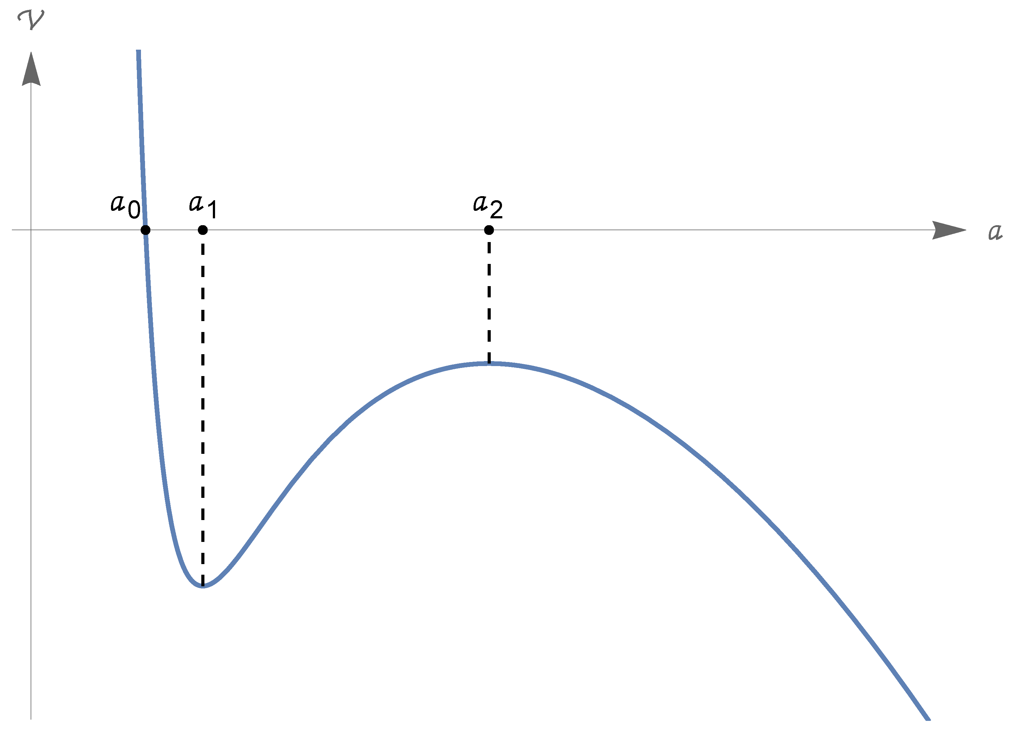
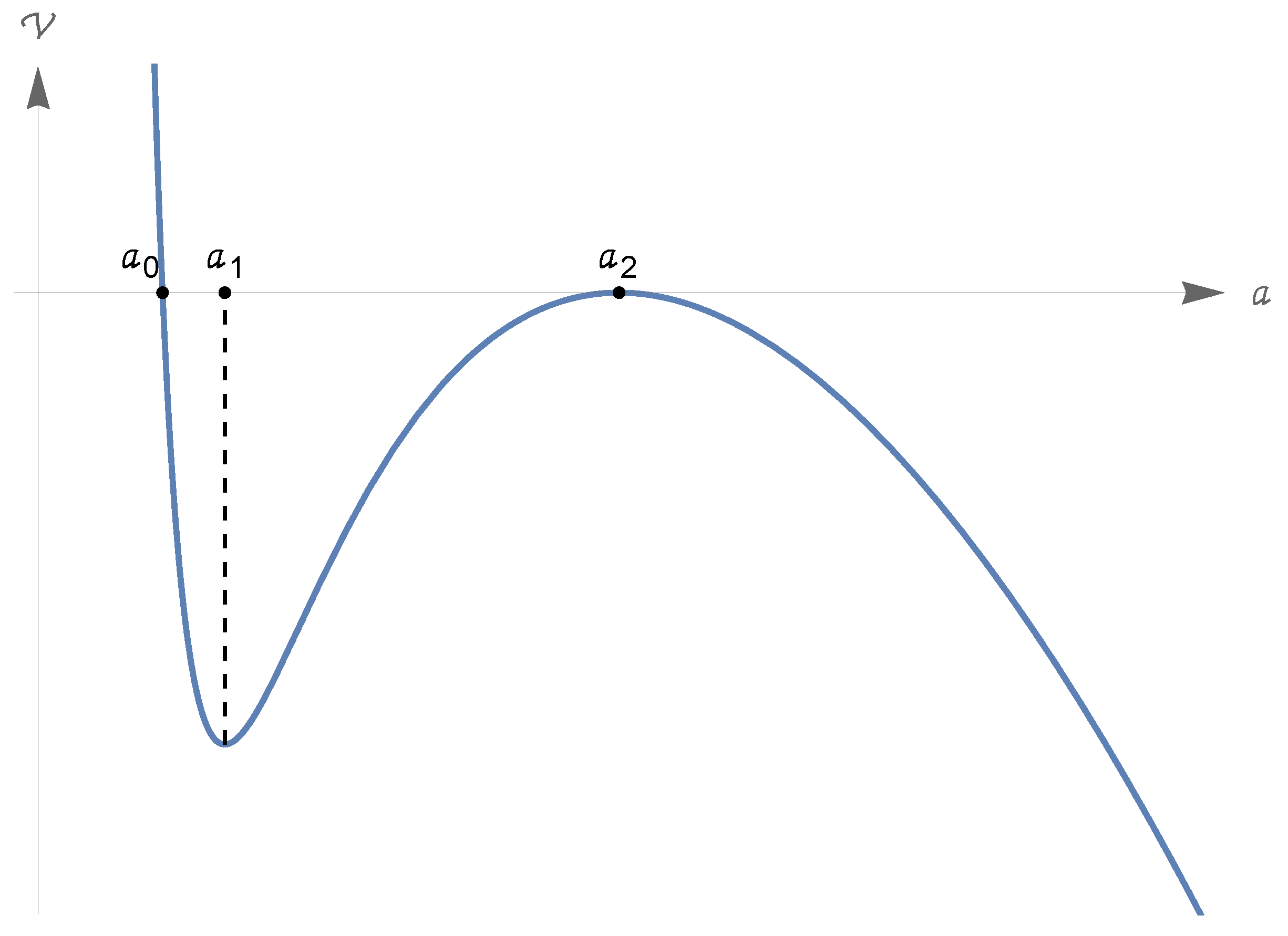
- We have the equivalenceIn the case (324), there is a unique point such that(i.e., has just two zeroes in ). We have again the inequality (322) . Moreover,(see Figure 6).
- ()
- We have the equivalence
- ()
- In any one of the cases ()–(), we have again the inequality (207) .
- ()
- Letthen, and . Moreover, in any one of the cases ()–(), we have
- Under the assumption (320), we have and . The behavior of a (maximal) zero-energy solution is similar to that described in the previous Section 6.6. So, is defined on the whole real axis with image . There is a Big Bounce at a time that we take conventionally to be , with ; moreover, and (exponentially) for .
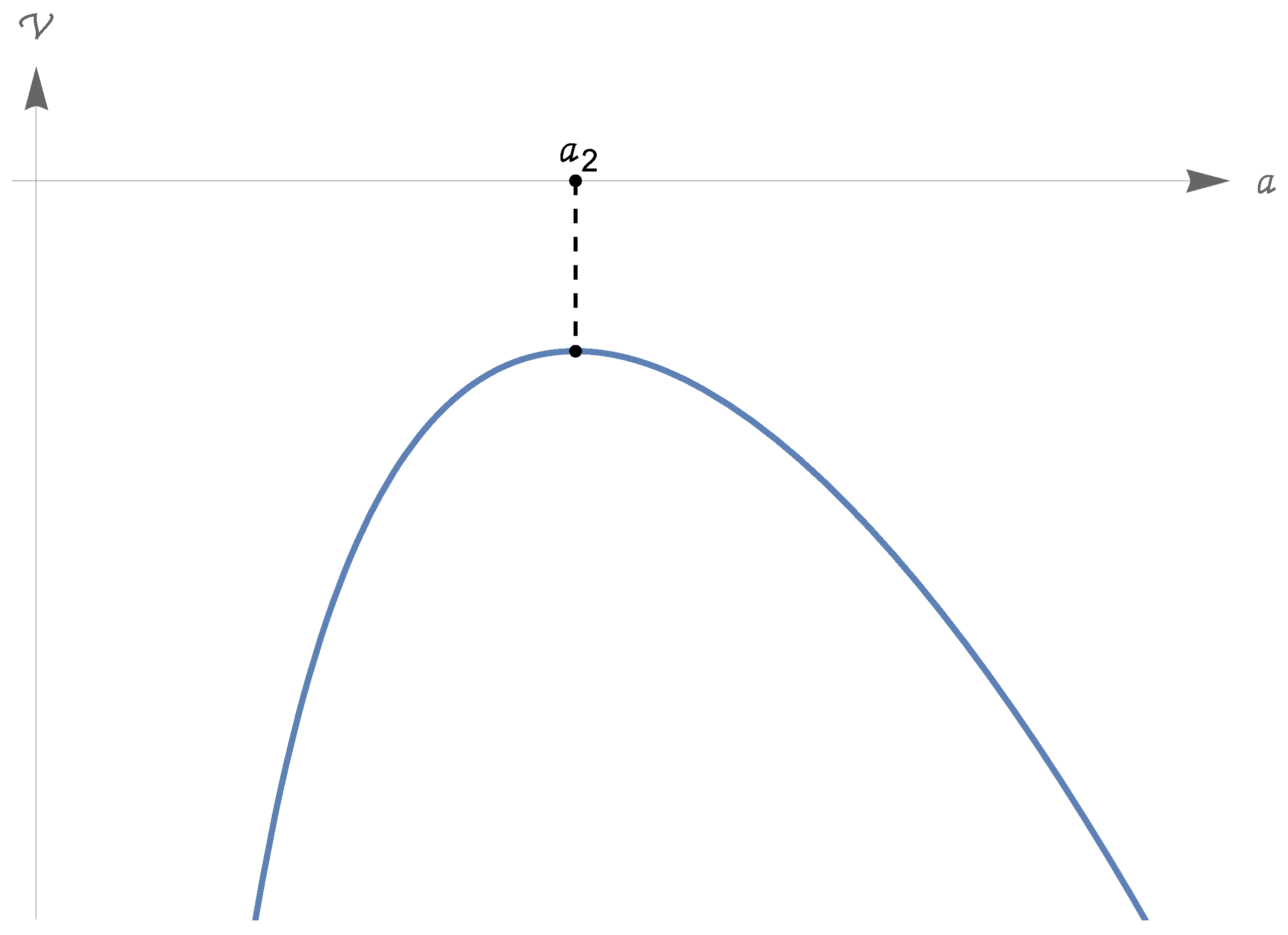
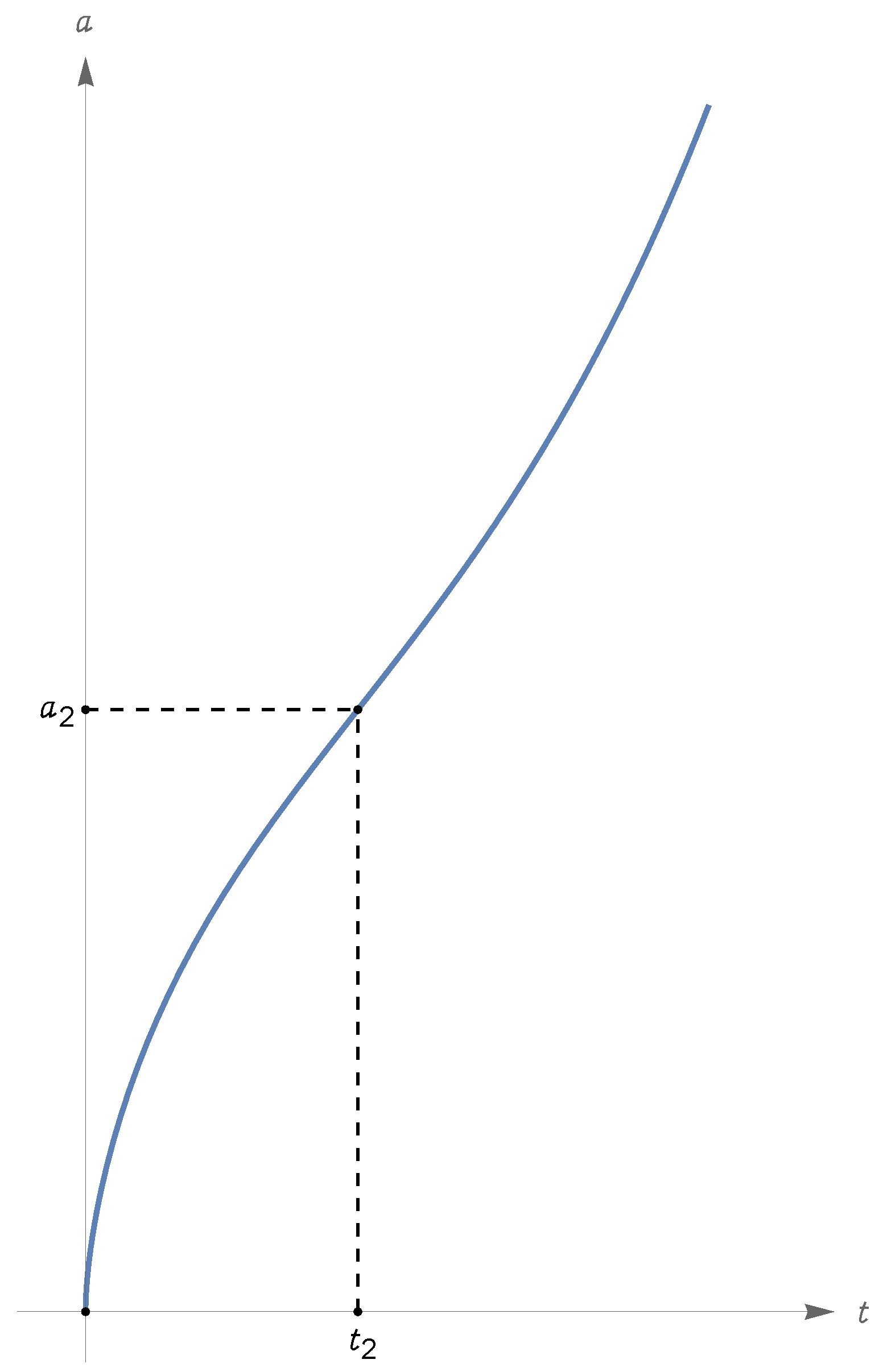
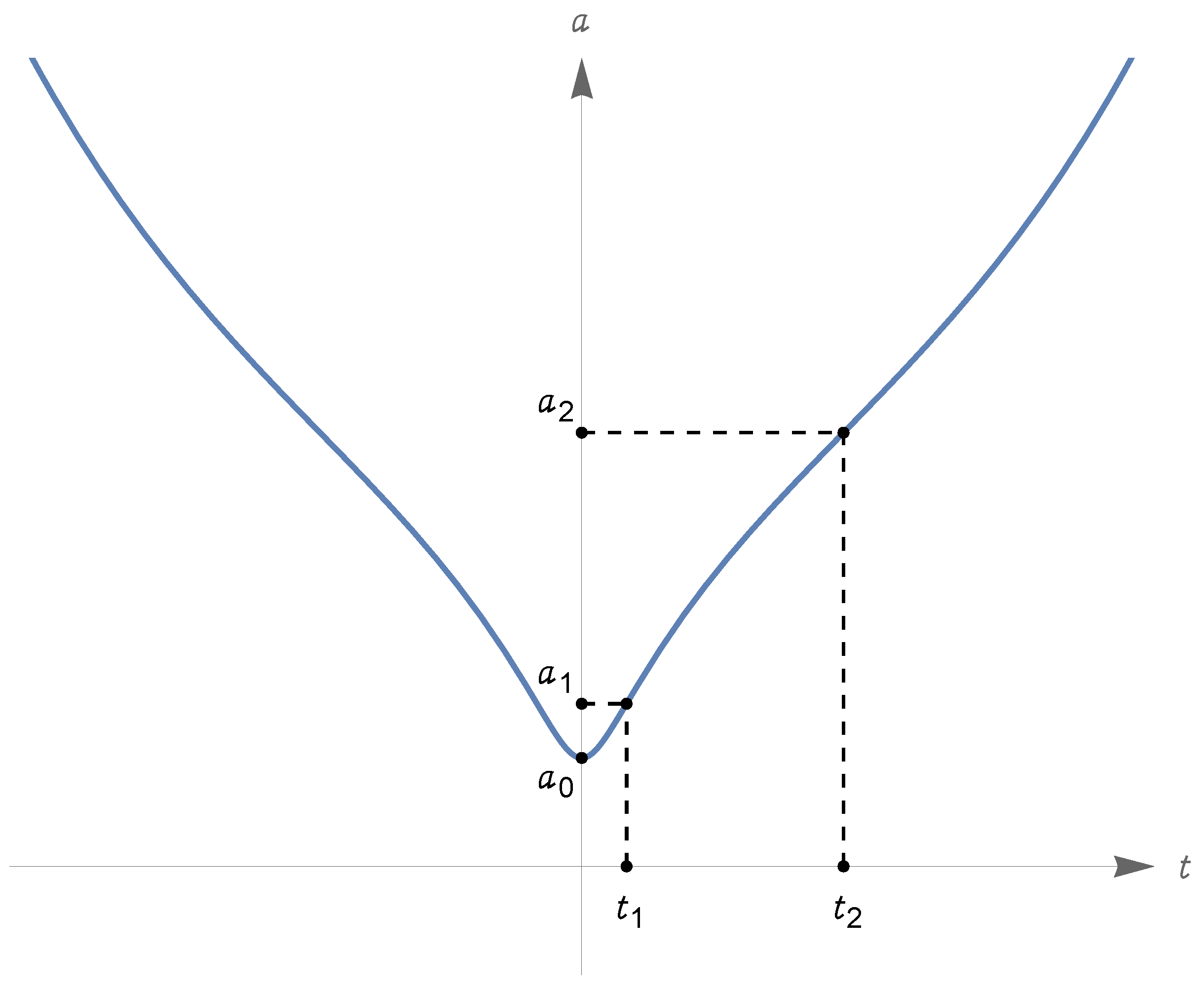
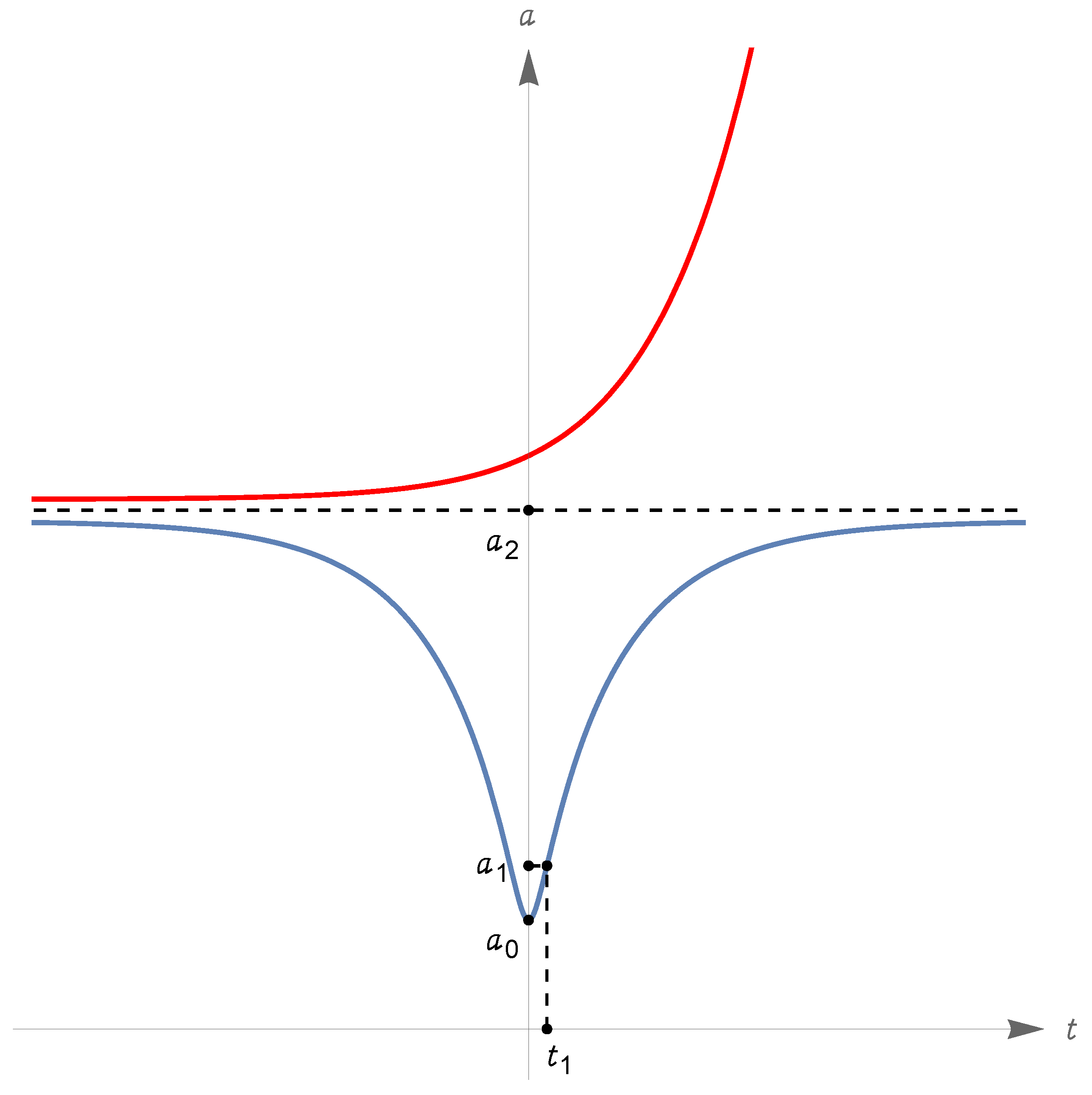
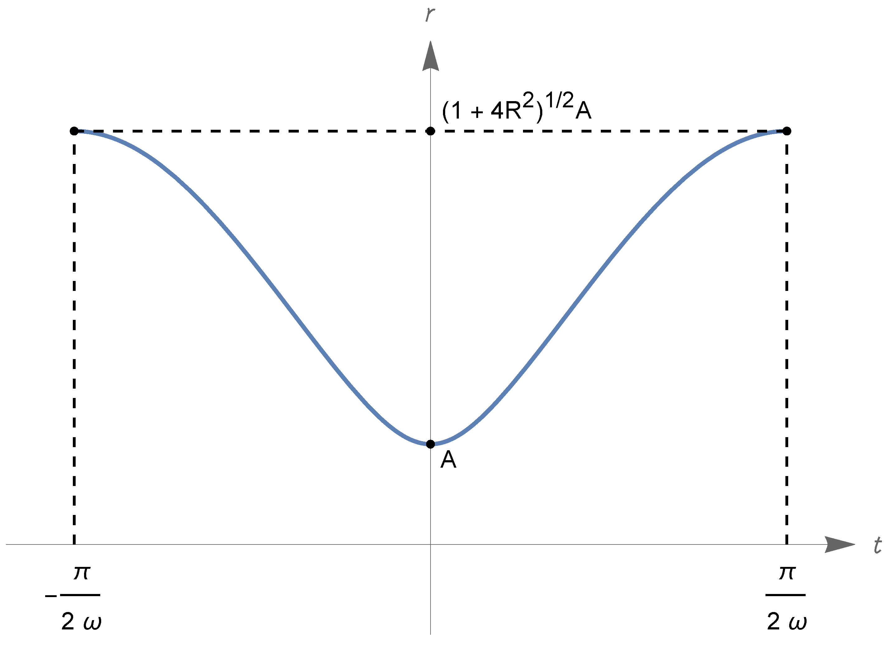
- Under the assumption (324), we have and , with and ; there are three types of zero-energy solutions, described hereafter.First type: There is a Big Bounce at , and is approached in the past and the future. We can assume the Big Bounce to occur at time , i.e., ; then, for all t. The function increases from to for and decreases from to for . The value is attained at times (see item (vi) in Section 5.4). In conclusion, has domain , range and . See Figure 8, where we also indicated the time such that ; recalling item (viii) in Section 5.4, we see that is an inflection point for the scale factor since and has different signs on the left and on the right of .Second type: has domain and range ; for all real t, or for all real t. If , we have for and for ; if , the values of the limits for are interchanged (the reason why the time required to reach is infinite is explained again by item (vi) in Section 5.4; the discussion of the time required for to diverge is related to item (vii) in the same section). In Figure 8, we illustrate the case .Third type: This corresponds to the equilibrium solution for all (see item (v) in Section 5.4).
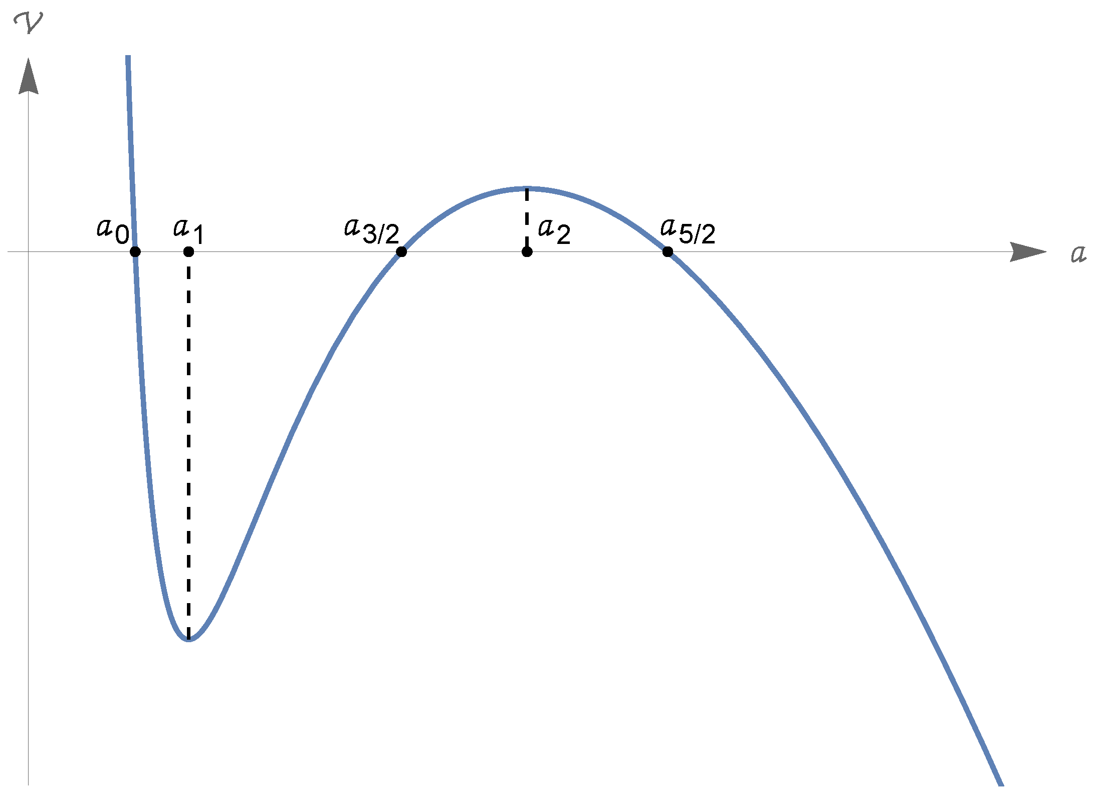
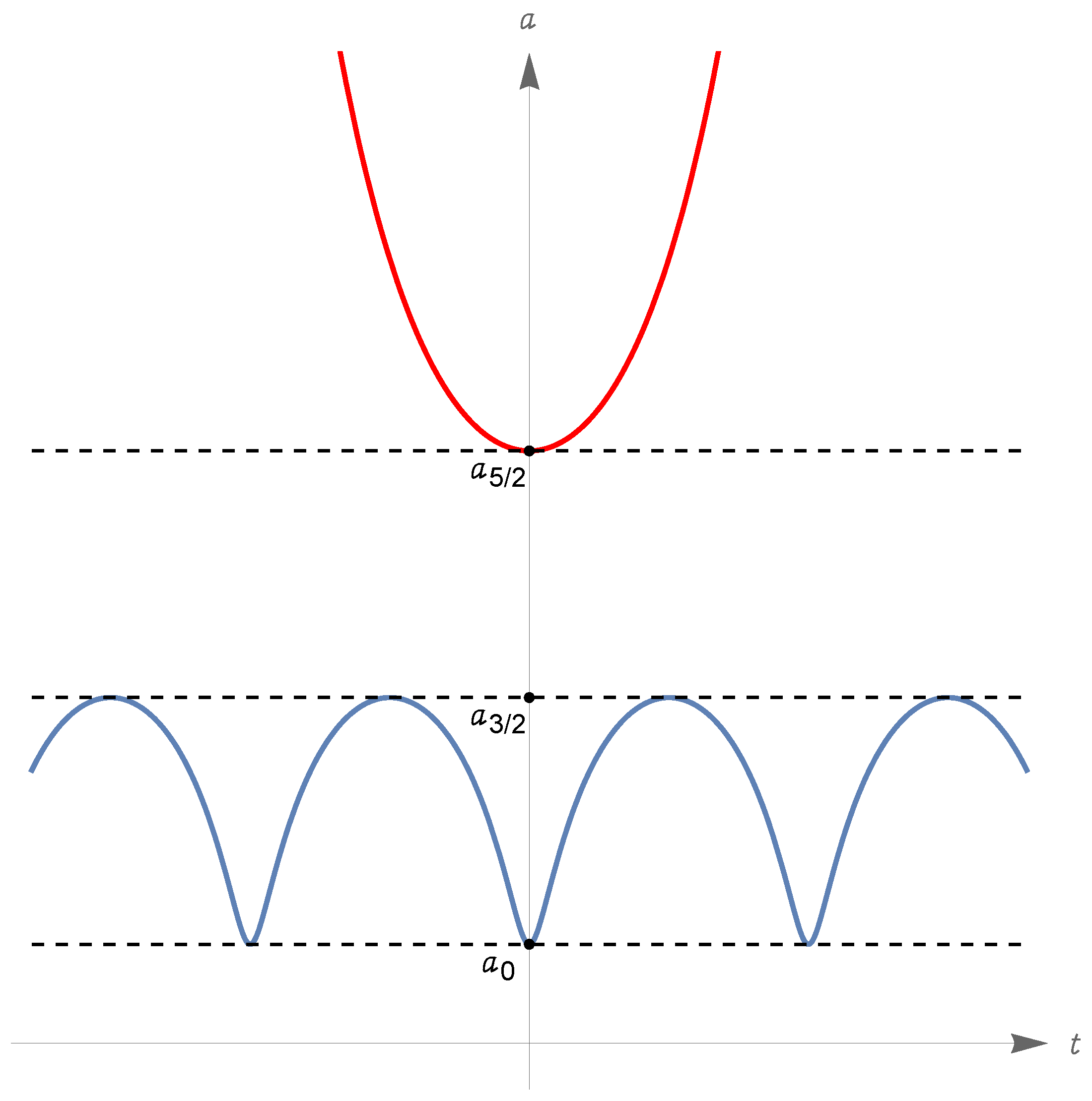
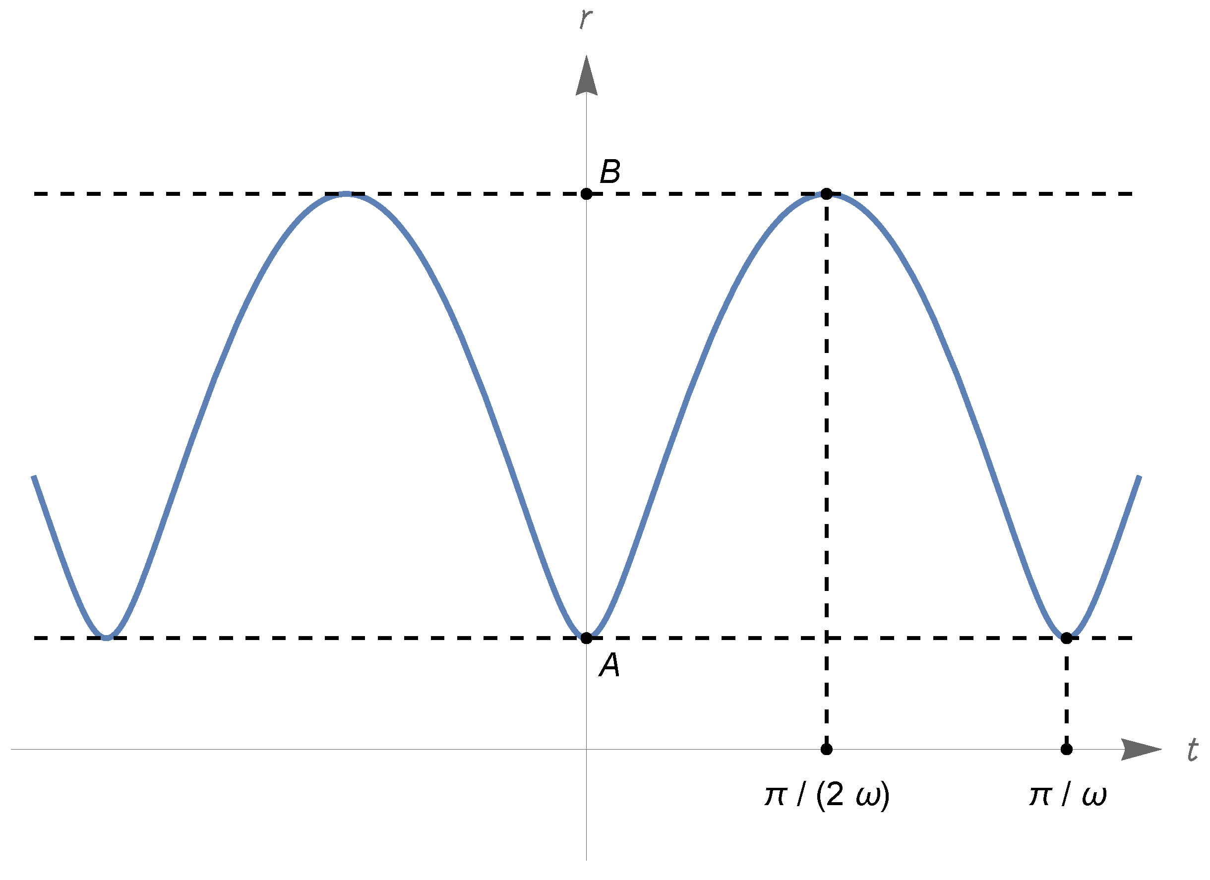
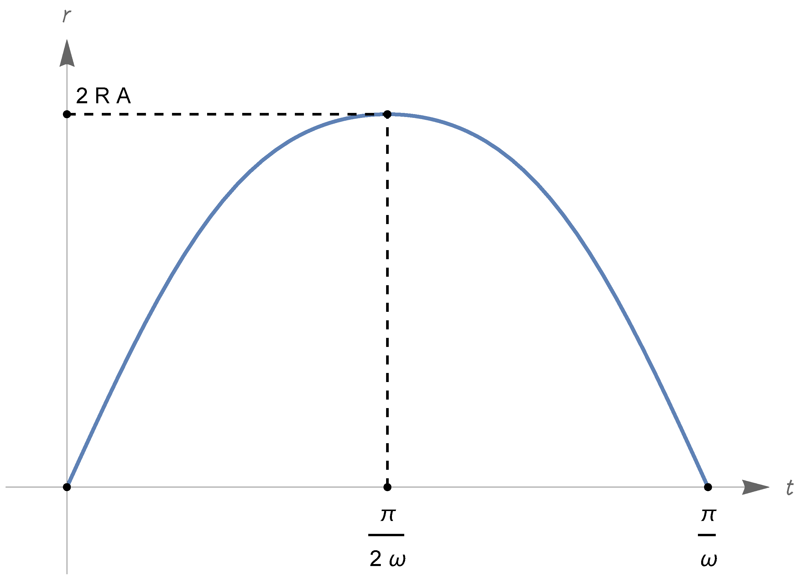
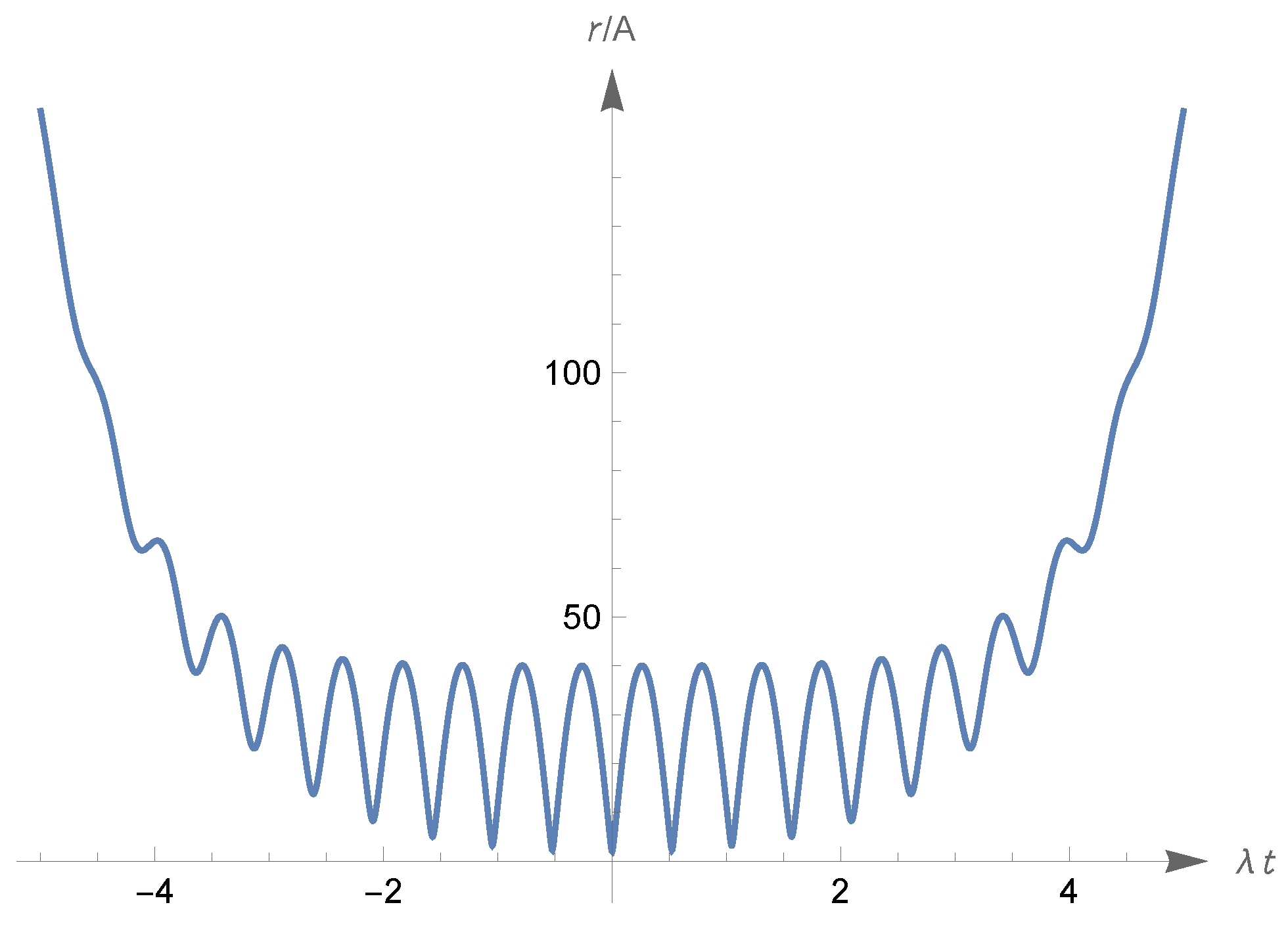
- Under the assumption (327), we have and , with , and ; there are two types of zero-energy solutions, described hereafter.First type: The function has domain and range ; it oscillates periodically with period(see items (ii)–(iv) in Section 5.4; the above convergent integral gives the time required for the scale factor to pass from to , that equals the time to return to ). This type of motion is represented in Figure 9 (note that the function has inflection points at the infinitely many times t such that ; these times are not indicated in the figure).Second type: The function has domain and range . There is a Big Bounce at the time when equals , which we can assume to be ; we have for all real t, is strictly increasing (resp., decreasing) on (resp., on ), and (exponentially) for . See Figure 9 again.
- In all the cases considered above, we have a cosmology with the time domain , in which the scale factor admits a strictly positive infimum. This is nonsingular in all senses considered in Section 3.2 and Section 3.15 (let us recall again Equation (69) and the related comments).
- Since the very beginning of the present study on cosmological models with matter, radiation, and a scalar field with constant self-potential, we have focused on the zero-energy solutions of the reduced system fulfilling at some time the condition , which is indeed equivalent to : see the discussion after Equation (177). Such a condition can either hold or fail for the solutions described above. For example, in the case (327), the requirement that at some time is fulfilled by the zero-energy solutions of the first type if and only if , and the zero-energy solutions of the second type if and only if .
7. Polar and Cartesian Coordinates for Phantom Cosmologies with a Periodic Field Potential
7.1. Polar Coordinates (Under Periodicity Assumptions for the Field Potential)
7.2. Cartesian Coordinates
8. An Explicitly Solvable Phantom Model with Dust and a Trigonometric Field Potential
8.1. Some Introductory Considerations
8.2. Introducing the Solvable Model
- There is only one perfect fluid of the dust type, i.e., with zero pressure. Thus,(to determine the expression of , we used Equation (114) with ); in the sequel we refer to this fluid with the generic denomination of “matter”. We assume the spatial curvature vanishes, so
- The function of Equation (337), giving the potential of the scalar field in terms of the coordinate , is assumed to have the form
8.3. The Case ()
8.4. Cosmologies with
- (i)
- We have
- (ii)
- We have
- (iii)
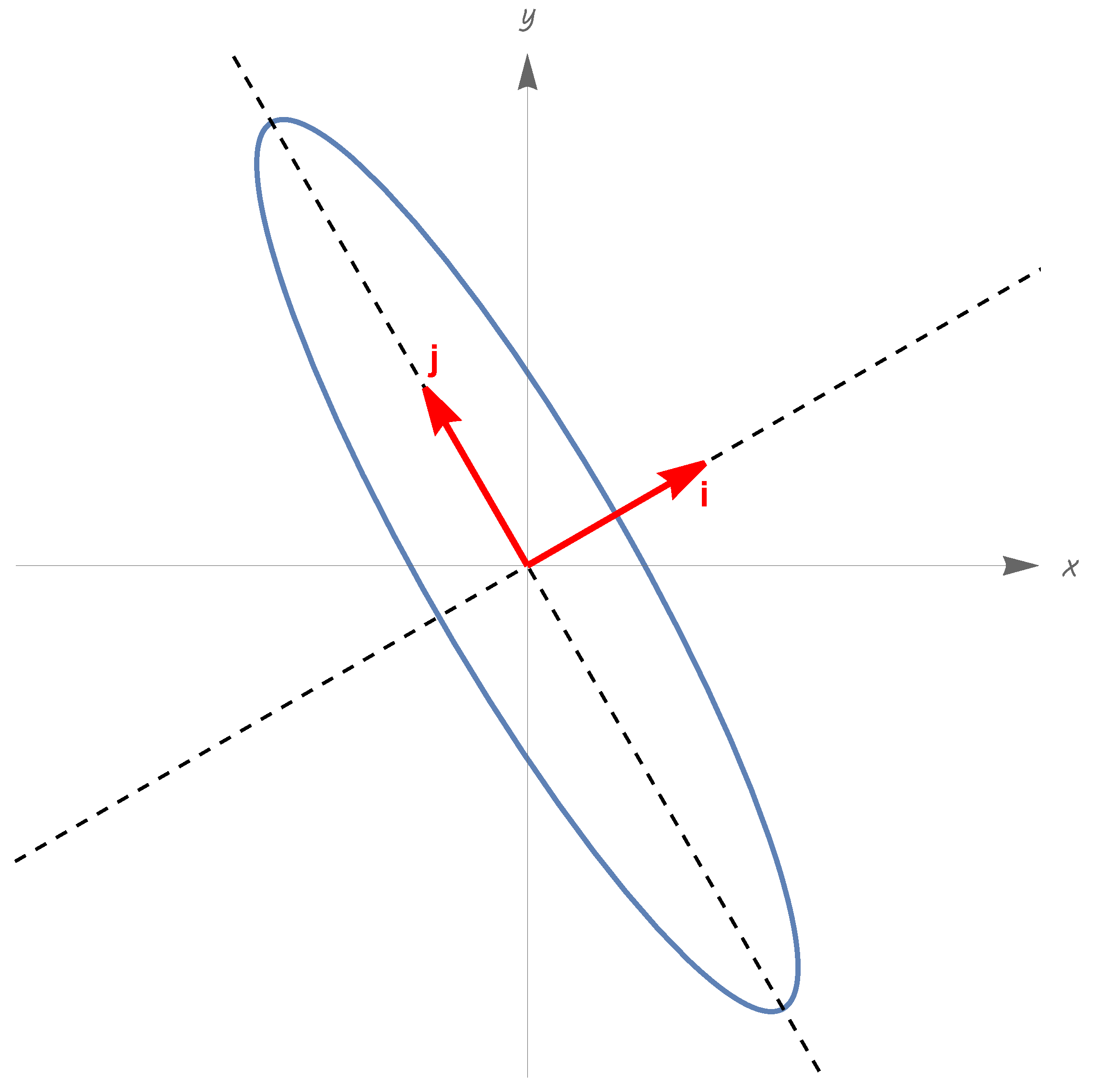
- Up to a time translation const., we havewhere( is the standard inner product of ; the previous conditions on indicate that this pair is an orthonormal basis of ).
8.5. Cosmologies with and Arbitrary
8.6. The Case (): Lissajous Cosmologies
8.7. Lissajous Cosmologies with
8.8. Lissajous Cosmologies with
8.9. On General Lissajous Cosmologies
- In rational case, where , the model is singular in any one of the senses considered in Section 3.2 and Section 3.15: in fact, any one of conditions (65)–(68) is violated (of course the times in the cited equations coincide with and , respectively).
8.10. The Case
8.11. Again on the Case ,
9. Concluding Remarks
Author Contributions
Funding
Data Availability Statement
Acknowledgments
Conflicts of Interest
Appendix A. Riemannian Manifolds, Spacetimes, and Dimensional Analysis
Appendix B. FLRW Spacetimes and Generalizations
Appendix C. Time Orientation of a Spacetime: The Case of a Generalized FLRW Spacetime
Appendix D. A Review on Geodesics and Several Associated Notions of Completeness, Mainly in Riemannian Manifolds and in Spacetimes. Nonsingular Spacetimes
- Past timelike complete if each maximal, future-directed timelike geodesic is past complete;
- Past lightlike complete if each maximal, future-directed lightlike geodesic is past complete;
- Past complete if it is both past timelike and past lightlike complete.
Appendix E. Geodesics and Geodesic Completeness of Generalized FLRW Spacetimes
- (i)
- is past timelike complete if and only ifIf all maximal, future-directed timelike geodesics are past incomplete. If and all maximal, future-directed timelike geodesics with nonconstant projection on are past incomplete.
- (ii)
- is past lightlike complete if and only if(note that (A69) does not require to be ).If all maximal, future-directed and nonconstant lightlike geodesics are past incomplete.
- (iii)
- is future timelike complete if and only ifIf all maximal, future-directed timelike geodesics are future incomplete. If and all maximal, future-directed timelike geodesics with nonconstant projection on are future incomplete.
- (iv)
- is future lightlike complete if and only if(note that (A71) does not require to be ).If all maximal, future-directed and nonconstant lightlike geodesics are future incomplete.
Appendix F. A Review the Energy Conditions
Appendix G. On the Determination of the Fluids’ Densities
Appendix H. Comparing the Zero Energy Motions of Two One-Dimensional Lagrangians
Appendix I. The Descartes’ Rule of Signs
Appendix J. Two Statements on a Class of Polynomials
- (i)
- LetThen, is well defined, and
- (ii)
- In addition, assumeand putThen, is well defined, and
Appendix K. Proof of Statements (185) and (186) on the Potential of the Standard Cosmological Model
Appendix L. Proof of Statements (a)–(d) in Section 6.5 about the Function of Equation (201)
Appendix M. Proof of Statements (f)–(i) in Section 6.5 about the Function of Equation (220)
Appendix N. Proof of Equation (250) (Including Convergence of an Integral Therein)
Appendix O. Proof of Some Statements about in Equation (271)
Appendix P. A Usefulf Inequality
Appendix Q. Estimates on the Time in Equation (244)
Appendix R. Further Estimates on the Time in Equation (244)
- According to (249), the time corresponds to the value of the scale factor; of course, we can set .
Appendix S. On the Quantity in Equation (292)
Appendix T. A More Detailed Description of the Model in Section 6.7
Appendix U. Proof of Statements (-) in Section 6.8 about the Function of Equation (201)
Appendix V. Derivation of Equations (363)–(366)
- (i)
- We have
- (ii)
- We have
- (iii)
- We havewhere(, are the standard norm and inner product of ).
Appendix W. Derivation of Equations (401) and (402)
| 1 | In models with a cosmological constant , the Einstein equations must be rephrased as with ; the energy conditions of the singularity theorems are required to hold for . The term individually fulfills the weak energy condition if and only if , and the strong energy condition if and only if . |
| 2 | Such tensorial constructions are described with great detail in two books by Matolcsi [65,66]. A technically different approach is developed in a paper by Janiška, Modugno, and Vitolo [67] and also sketched in a subsequent book by Janiška and Modugno [68]; these authors focus on the notion of one-dimensional semi-vector space, which can be interpreted as the positive part of a one-dimensional, oriented vector space. |
| 3 | In the general framework of Section 2, Section 3, Section 4 and Section 5 and Section 7, the fluids are not required to fulfill the usual (e.g., the weak or strong) energy conditions; however this happens in the applications of Section 6 and Section 8, where the fluids are in fact dust or a radiation gas. |
| 4 | Let us add some detail. A history of the n-th fluid is a congruence of timelike curves in ; such curves, one through any spacetime point, represent the world lines of the fluid’s particles. A history of the fluid determines a mass density , describing the spacetime distribution of the particles’ masses due to their motions. The fluid also possesses a (constitutive, history-independent) function , representing an elastic potential per unit mass; given a history with mass density , the corresponding mass–energy density is . Concerning the previous issues, see Section 3.3, Example 4 of the cited book [12] (this reference considers a single fluid, calling the mass density and the mass–energy density; here, we interchange the letters used for the two densities. The same reference considers the congruences of timelike curves without using the denomination of histories, which, however, is generally employed in variational calculus). |
| 5 | Let us add a comment on the pressures appearing in Equation (8). Variational calculations performed as in Section 3.3, Example 4 of [12], give the pressure of each fluid as a function of the mass density , determined by the elastic potential (see the previous note). More precisely, we have , where ′ is the derivative. We know that (see again the previous note); assuming that this relation can be inverted, we finally obtain as a function of , as in Equation (5). For example, if with two given constants , , we finally obtain . |
| 6 | Obviously enough, the previous considerations can be generalized to the case where we have a decomposition , with a constant and any smooth function. In this case, the Einstein equations can be put in the form (13), where the cosmological constant is given again by Equation (14), and is the stress–energy tensor of a scalar field with self-potential . |
| 7 | Appendix B also introduces the notion of generalized FLRW spacetime, which is used in some of the subsequent appendices and allows us to draw links with some of the references cited in the present work. However, in the main text of the present paper we always refer to an ordinary FLRW spacetime, as described in Section 3.1. |
| 8 | The notions of timelike and lightlike completeness date back to the pioneering works in this area; see, e.g., [44]. The definition of a nonsingular spacetime adopted in this work, based on the requirements of timelike and lightlike completeness, can be found in [12] (page 258). Other authors (see, e.g., [45] (page 215)) also require spacelike completeness, meaning that the maximal spacelike geodesics have domain ; we briefly return to this point in the subsequent note. |
| 9 | The results in the cited papers apply to a class of generalized FLRW spacetimes, described in Appendix B and Appendix E; as already indicated, the main text of the present work will only consider the usual FLRW spacetimes of Section 3.1. The studies [61,62] also prove the following result: if a generalized FLRW spacetime is lightlike complete, it is as well spacelike complete (in the sense of the previous note). |
| 10 | |
| 11 | |
| 12 | This expression for and the subsequent one for follow easily from the standard rules for the coordinate representation of covariant derivatives, as well as from the expressions for the Christoffel symbols of the spacetime metric reported in Appendix B. |
| 13 | The rest of the paper makes more and more clear that there are analogies between the fluids’ densities and the curvature density ; this is why, in Equation (46) and in many subsequent formulas, the term corresponding to the curvature density is written immediately after the terms related to the fluids’ densities. |
| 14 | |
| 15 | Let us recall Equation (26), and the note that accompanies it. |
| 16 | For a direct check, one can use the identity . Due to this identity, and ⇒ = constant; thus, , and at some time ⇒ (at all times). |
| 17 | By the standard theory of the Cauchy problem, this solution exists and is unique if we require it to be maximal, in the sense of the subsequent Section 4.6. |
| 18 | All figures presented in this paper were produced using Mathematica (version 12.3) by Wolfram Research Inc. (Champaign, Illinois); the same package was employed for all numerical computations. |
| 19 | The occurrence of a Big Bang in case (iii) is derived by the methods of Section 5.4 for the qualitative description of one-dimensional conservative systems. The essential reason for the Big Bang is the same holding for the standard model: for small a, decreases to . (As in the standard model, the singularity at is attained at a finite time since vanishes for , and thus is integrable in a right neighborhood of zero.) That said, let us remark that the asymptotics of is different in the two cases: in this limit, we have in the standard case (see Equation (184)), while (due to (168)) in case (iii); these facts imply different laws for the growth of the scale factor immediately after the Big Bang. |
| 20 | Let us consider the standard model with positive cosmological constant and, e.g., with nonpositive spatial curvature, displaying a Big Bang at time . In this case, we also have after a suitable time ; see Section 6.2. However, in this model, the SEC holds close to ; according to the singularity theorems mentioned in the Introduction, this is just the reason why the model presents a Big Bang! |
| 21 | One could argue that the condition justifying the classical treatment of gravity is , where is the total density without the curvature contribution . The discussion of this issue is nontrivial; regardless, in the application of the classicality condition presented in this paper (see Section 6.7), the spatial curvature vanishes, so that . |
| 22 | Of course the idea to put a condition on a cosmological model based on the Planck units, so as to justify the classical treatment of gravity, is not at all new: see, e.g., the condition on the Riemann curvature tensor presented after Equations (2) and (3) in [54]. |
| 23 | |
| 24 | Of course, the above expressions of via radicals are obtained noting that the cubes of these quantities fulfill algebraic equations of degree two. We could also express , via radicals, noting that their squares fulfill algebraic equations of degree three and using the Cardano formula. |
| 25 | |
| 26 | The cited Equation (197) also reports the value of a time , indistinguishable from the homonymous value in Equation (310). Indeed, after an extremely short time-lapse from the Big Bounce, the present model (with nonzero but extremely small ) becomes quantitatively indistinguishable in several aspects from the standard model (corresponding to ). |
| 27 | Here, we do not consider the values of a involved in comparisons with the curvature density , since the latter vanishes. |
| 28 | Let us repeat that all numerical computations mentioned in this paper were performed using Mathematica (version 12.3). |
| 29 | Here and in the sequel, is the set of relative integers. For each , we denote with the one-dimensional torus of period P, i.e., the quotient of with respect to the relation of equivalence mod. P (two real numbers are equivalent mod. P if there is such that ). For each , we often write (mod. P) for the equivalence class containing ; thus, (mod. P) . |
| 30 | For each , the quotient is defined like the quotient of the previous note, replacing with and P with F. |
| 31 | |
| 32 | See, in particular, Equation (19) of [25]; essentially, this can be re-obtained from our Equations (350) and (351) for the field potential setting . Let us also mention that our Cartesian coordinates have a role similar to the coordinates of [25] (more precisely, our variables are analogs for const. u and const. ). In our approach, (polar and) Cartesian coordinates are a rather natural choice in the Lagrangian setting, which subsequently results in individuating the potential (350) and (351) as one giving a solvable model. On the contrary, the potential of [25] and the coordinates used therein were individuated by applying the theory of Nöther symmetries to the general Lagrangian formalism for a phantom scalar in the presence of dust. |
| 33 | All works [26,27,28,30,31,32] consider a canonical scalar field with a potential that can be expressed in the dimensionless form , with a suitable normalization constant; V has a slightly different exponential form in [77] (where this model is considered for a peculiar reason: it is a preliminary step in the construction of an FLRW cosmology with degenerate, signature changing spacetime metric). Hereafter, with , we indicate the separation coordinates in any one of the cited papers; these can be interpreted as orthonormal coordinates on the two-dimensional Minkowski space, in which the line element reads . The scale factor of the corresponding cosmological model is expressed as const. , and this formula replaces our expression const. const. (see the present Equations (335) and (344)). So, the trajectories in the -space of [26,27,28,30,31,32,77] and the trajectories in the -space of the present paper have different cosmological meanings. |
| 34 | The model of [77] with a canonical scalar field and an exponential self-interaction also appears in a recent review by Jalalzadeh, Rasouli, and Moniz [78] on supersymmetric quantum cosmology, where it is considered for application of the Wheeler–DeWitt equation; the cited review mentions (with no analysis of the cosmological implications) that the uncoupled harmonic oscillators resulting from the model produce Lissajous curves. For the reasons indicated previously, the Lissajous curves of [78] and those considered in the present work have different cosmological interpretations. |
| 35 | See Section 8.9, and the subsequent note on the case . |
| 36 | For example, if , we have and , so that . This confirms the statements after Equation (430). |
| 37 | Here is the proof of the uniqueness of the zero of . Let be two times such that . According to Equations (446)–(448), we have and for some . These facts imply , i.e., by the explicit expressions in (446) and (447), . Due to the last equality, and are both nonvanishing or both vanishing. If it were and , we could infer from the last equality that , against the assumption that is irrational. Thus, and ; these equalities imply and , whence . |
| 38 | |
| 39 | The divergence of the integral in Equation (67) is checked by arguments very similar to those employed in the previous note. |
| 40 | For , and (), it turns out that if and only if (), with . As a domain for the corresponding cosmological model, we can assume any interval of the form , for example, the interval ; the model has a Big Bang at and a Big Crunch at . |
| 41 | In the present case, the ends of the time domain are , as required by Equations (65) and (67). The verification of the other nonsingularity conditions is simple; the less obvious statement is the divergence of the integral in Equation (65), where is arbitrarily chosen. In order to clarify this point, after fixing , we note that Equation (467) implies
|
| 42 | |
| 43 | Needless to say, the coordinate description of is defined for such that is in the domain of the coordinate system. In Equation (A21), indicates the map . One could make similar comments on other expressions, appearing in Appendix D and Appendix E. |
| 44 | Of course, the distance between two points in the infimum of the lengths of the (piecewise smooth) curves joining the points, defining such lengths via h. The equivalence between geodesic completeness and completeness in the distance induced by h is proved, e.g., in [83]. |
| 45 | A (parametrized) curve is said to be timelike, lightlike or spacelike if so is its velocity at any p. |
| 46 | |
| 47 | |
| 48 | |
| 49 | Here and in the rest of Appendix F, should be understood as abstract indexes in the sense of Penrose, while are concrete labels. |
| 50 | Even though for , we cannot grant a strict inequality in (A98) since could be empty. |
| 51 |
References
- Brans, C.; Dicke, H. Mach’s principle and a relativistic theory of gravitation. Phys. Rev. 1961, 124, 925–935. [Google Scholar] [CrossRef]
- Linde, A.D. Chaotic inflation. Phys. Lett. B 1983, 129, 177–181. [Google Scholar] [CrossRef]
- Madsen, M.S.; Coles, P. Chaotic Inflation. Nucl. Phys. B 1988, 298, 701–725. [Google Scholar] [CrossRef]
- Ratra, B.; Peebles, P.J.E. Cosmological consequences of a rolling homogeneous scalar field. Phys. Rev. D 1988, 37, 3406–3427. [Google Scholar] [CrossRef]
- Caldwell, R.R.; Dave, R.; Steinhardt, P.J. Cosmological imprint of an energy component with general equation of state. Phys. Rev. Lett. 1998, 80, 1582–1585. [Google Scholar] [CrossRef]
- Peebles, P.J.E.; Vilenkin, A. Quintessential inflation. Phys. Rev. D 1999, 59, 063505. [Google Scholar] [CrossRef]
- Bekenstein, J.D. Nonsingular general-relativistic cosmologies. Phys. Rev. D 1975, 11, 2072–2075. [Google Scholar] [CrossRef]
- Parker, L.E.; Toms, D.J. Quantum Field Theory in Curved Spacetime: Quantized Fields and Gravity; Cambridge University Press: Cambridge, UK, 2009. [Google Scholar]
- Avsajanishvili, O.; Chitov, G.Y.; Kahniashvili, T.; Mandal, S.; Samushia, L. Observational Constraints on Dynamical Dark Energy Models. Universe 2024, 10, 122. [Google Scholar] [CrossRef]
- Saini, T.D.; Raychaudhury, S.; Sahni, V.; Starobinsky, A.A. Reconstructing the Cosmic Equation of State from Supernova Distances. Phys. Rev. Lett. 2000, 85, 1162–1165. [Google Scholar] [CrossRef]
- Perlmutter, S.; Aldering, G.; Goldhaber, G.; Knop, R.A.; Nugent, P.; Castro, P.G.; Deustua, S.; Fabbro, S.; Goobar, A.; Groom, D.E.; et al. Measurements of Omega and Lambda from 42 high redshift supernovae. Astrophys. J. 1999, 517, 565–586. [Google Scholar] [CrossRef]
- Hawking, S.W.; Ellis, G.F.R. The Large Scale Structure of Space-Time; Cambridge University Press: Cambridge, UK, 1975. [Google Scholar]
- Maeda, H.; Martínez, C. Energy conditions in arbitrary dimensions. Prog. Theor. Exp. Phys. 2020, 2020, 043E02. [Google Scholar] [CrossRef]
- Fermi, D.; Pizzocchero, L. Local Zeta Regularization and the Scalar Casimir Effect. A General Approach Based on Integral Kernels; World Scientific Publishing, Co.: Singapore, 2017. [Google Scholar]
- Fermi, D.; Pizzocchero, L. On the Casimir effect with δ-like potentials, and a recent paper by Ziemian, K. Ann. Henri Poincaré 2023, 24, 2363–2400. [Google Scholar] [CrossRef]
- Nojiri, S.; Odintsov, S.D. Quantum de Sitter cosmology and phantom matter. Phys. Lett. B 2003, 562, 147–152. [Google Scholar] [CrossRef]
- Ellis, H. Ether flow through a drainhole: A particle model in general relativity. J. Math. Phys. 1973, 14, 104–118. [Google Scholar] [CrossRef]
- Bronnikov, K.A. Scalar-tensor theory and scalar charge. Acta Phys. Polon. 1973, B4, 251–266. [Google Scholar]
- Caldwell, R.R. A phantom menace? Cosmological consequences of a dark energy component with super-negative equation of state. Phys. Lett. B 2002, 545, 23–29. [Google Scholar] [CrossRef]
- Carroll, S.M.; Hoffman, M.; Trodden, M. Can the dark energy equation-of-state parameter w be less than −1? Phys. Rev. D 2003, 68, 023509. [Google Scholar] [CrossRef]
- Capozziello, S.; Nojiri, S.; Odintsov, S.D. Unified phantom cosmology: Inflation, dark energy and dark matter under the same standard. Phys. Lett. B 2006, 632, 597–604. [Google Scholar] [CrossRef]
- Elizalde, E.; Nojiri, S.; Odintsov, S.D.; Sáez-Gómez, D.; Faraoni, V. Reconstructing the universe history, from inflation to acceleration, with phantom and canonical scalar fields. Phys. Rev. D 2008, 77, 106005. [Google Scholar] [CrossRef]
- Fermi, D.; Gengo, M.; Pizzocchero, L. On the necessity of phantom fields for solving the horizon problem in scalar cosmologies. Universe 2019, 5, 76. [Google Scholar] [CrossRef]
- Faraoni, V. Cosmology in Scalar-Tensor Gravity; Kluwer Academic Publishers: Dohrdrecht, The Netherlands, 2004. [Google Scholar]
- Capozziello, S.; Piedipalumbo, E.; Rubano, C.; Scudellaro, P. Noether symmetry approach in phantom quintessence cosmology. Phys. Rev. D 2009, 80, 104030. [Google Scholar] [CrossRef]
- de Ritis, R.; Marmo, G.; Platania, G.; Rubano, C.; Scudellaro, P.; Stornaiolo, C. New approach to find exact solutions for cosmological models with a scalar field. Phys. Rev. D 1990, 42, 1091–1097. [Google Scholar] [CrossRef] [PubMed]
- Piedipalumbo, E.; Scudellaro, P.; Esposito, G.; Rubano, C. On quintessential cosmological models and exponential potentials. Gen. Rel. Grav. 2012, 44, 2611–2643. [Google Scholar] [CrossRef]
- Rubano, C.; Scudellaro, P. On some exponential potentials for a cosmological scalar field as quintessence. Gen. Rel. Grav. 2002, 34, 307–327. [Google Scholar] [CrossRef]
- Capozziello, S.; de Ritis, R.; Rubano, C.; Scudellaro, P. Nöther symmetries in cosmology. Riv. Nuovo C. 1996, 19, 1–114. [Google Scholar] [CrossRef]
- Fré, P.; Sagnotti, A.; Sorin, A.S. Integrable scalar cosmologies, I. Foundations and links with string theory. Nucl. Phys. B 2013, 877, 1028–1106. [Google Scholar] [CrossRef]
- Gengo, M. Integrable Multidimensional Cosmologies with Matter and a Scalar Field. Ph.D. Thesis, Doctoral Program in Mathematical Sciences, Università degli Studi di Milano, Milano, Italy, 2019. Available online: https://air.unimi.it/handle/2434/613446 (accessed on 3 August 2024).
- Fermi, D.; Gengo, M.; Pizzocchero, L. Integrable scalar cosmologies with matter and curvature. Nucl. Phys. B 2020, 957, 115095. [Google Scholar] [CrossRef]
- Ellis, G.F.R.; Madsen, M.S. Exact scalar field cosmologies. Class. Quantum Gravity 1991, 8, 667–676. [Google Scholar] [CrossRef]
- Easther, R. Exact superstring motivated cosmological models. Class. Quantum Gravity 1993, 10, 2203–2215. [Google Scholar] [CrossRef]
- Dimakis, N.; Karagiorgos, A.; Zampeli, A.; Paliathanasis, A.; Terzis, P.A. General analytic solutions of scalar field cosmology with arbitrary potential. Phys. Rev. D 2016, 93, 123518. [Google Scholar] [CrossRef]
- Barrow, J.D.; Paliathanasis, A. Observational constraints on new exact inflationary scalar-field solutions. Phys. Rev. D 2016, 94, 083518. [Google Scholar] [CrossRef]
- Chervon, S.; Fomin, I.; Yurov, A. Scalar Field Cosmology; Series on the Foundations of Natural Science and Technology; World Scientific: Singapore, 2019; Volume 13. [Google Scholar]
- Ivanov, G.G. Friedmann cosmological model with nonlinear scalar field. Gravitaciya Teor. Otnos. 1981, 18, 54–60. Available online: http://www.stfi.ru/journal/STFI_2020_03/STFI_2020_03_Ivanov.pdf (accessed on 1 November 2024).
- Salopek, D.S.; Bond, J.R. Nonlinear evolution of long-wavelength metric fluctuations in inflationary models. Phys. Rev. D 1990, 42, 3936–3962. [Google Scholar] [CrossRef]
- Chervon, S.V.; Panina, O.G. The exact cosmological solutions for phantom fields. Vestn. Samar. Gos. Tekhn. Univ. Ser. Fiz.-Mat. Nauki 2011, 3, 129–135. [Google Scholar]
- Geroch, R.P. Singularities in closed universes. Phys. Rev. Lett. 1966, 17, 445–447. [Google Scholar] [CrossRef]
- Hawking, S.W. Occurrence of singularities in open universes. Phys. Rev. Lett. 1965, 15, 689–690. [Google Scholar] [CrossRef]
- Hawking, S.W.; Penrose, R. The singularities of gravitational collapse and cosmology. Proc. R. Soc. A 1970, 314, 529–548. [Google Scholar]
- Penrose, R. Gravitational collapse and space-time singularities. Phys. Rev. Lett. 1965, 14, 57–59. [Google Scholar] [CrossRef]
- Wald, R.M. General Relativity; The University of Chicago Press: Chicago, IL, USA, 1984. [Google Scholar]
- Novello, M.; Bergliaffa, S.E.P. Bouncing cosmologies. Phys. Rep. 2008, 463, 127–213. [Google Scholar] [CrossRef]
- Boisseau, B.; Giacomini, H.; Polarski, D.; Starobinsky, A.A. Bouncing universes in scalar-tensor gravity models admitting negative potentials. J. Cosmol. Astropart. Phys. 2015, 2015, 2. [Google Scholar] [CrossRef]
- Bekenstein, J.D. Exact solutions of Einstein-conformal scalar equations. Ann. Phys. 1974, 82, 535–547. [Google Scholar] [CrossRef]
- Dabrowski, M.P. Oscillating Friedman cosmology. Ann. Phys. 1996, 248, 199–219. [Google Scholar] [CrossRef]
- Dabrowski, M.P.; Stachowiak, T.; Szydlowski, M. Phantom cosmologies. Phys. Rev. D 2003, 68, 103519. [Google Scholar] [CrossRef]
- Dabrowski, M.P.; Stachowiak, T. Phantom Friedmann cosmologies and higher-order characteristics of expansion. Ann. Phys. 2006, 321, 771–812. [Google Scholar] [CrossRef]
- Parker, L.; Fulling, S.A. Quantized matter fields and the avoidance of singularities in general relativity. Phys. Rev. D 1973, 7, 2357–2374. [Google Scholar] [CrossRef]
- Starobinskii, A.A. On a nonsigular isotropic cosmological model. Sov. Astron. Lett. 1978, 4, 82–84. [Google Scholar]
- Starobinsky, A.A. A new type of isotropic cosmological models without singularity. Phys. Lett. 1980, 91, 99–101. [Google Scholar] [CrossRef]
- Gurovich, V.T.; Starobinsky, A.A. Quantum effects and regular cosmological models. Sov. Phys. JETP 1979, 50, 844–845. [Google Scholar]
- Anderson, P. Effects of quantum fields on singularities and particle horizons in the early universe. Phys. Rev. D 1983, 28, 271–285, Erratum in Phys. Rev. D 1983, 28, 2695. [Google Scholar] [CrossRef]
- Anderson, P. Effects of quantum fields on singularities and particle horizons in the early universe II. Phys. Rev. D 1984, 29, 615–625. [Google Scholar] [CrossRef]
- Dappiaggi, C.; Fredenhagen, K.; Pinamonti, N. Stable cosmological models driven by a free quantum scalar field. Phys. Rev. D 2008, 77, 104015. [Google Scholar] [CrossRef]
- Ashtekar, A.; Pawlowski, T.; Singh, P. Quantum nature of the Big Bang: An analytical and numerical investigation. Phys. Rev. D 2006, 73, 124038. [Google Scholar] [CrossRef]
- O’Neill, B. Semi-Riemannian Geometry with Applications to Relativity; Pure and Applied Mathematics Series; Academic Press: San Diego, CA, USA, 1983. [Google Scholar]
- Romero, A.; Sanchez, M. On the completeness of certain families of semi-Riemannian manifolds. Lett. Math. Phys. 1994, 53, 103–117. [Google Scholar] [CrossRef]
- Sanchez, M. On the geometry of generalized Robertson-Walker spacetimes: Geodesics. Gen. Relativ. Gravit. 1998, 30, 915–932. [Google Scholar] [CrossRef]
- Weisstein, E.W. Lissajous Curve. In MathWorld—A Wolfram Web Resource. Available online: https://mathworld.wolfram.com/LissajousCurve.html (accessed on 3 August 2024).
- Arnold, V.I. Mathematical Methods of Classical Mechanics; Graduate Texts in Mathematics; Springer: New York, NY, USA, 1989; Volume 60. [Google Scholar]
- Matolcsi, T. A Concept of Mathematical Physics. Models for Space-Time; Akadémiai Kiaidó: Budapest, Hungary, 1984. [Google Scholar]
- Matolcsi, T. Spacetime without Reference Frames, 2nd ed.; Society for the Unity of Science and Technology: Budapest, Hungary, 2018. [Google Scholar]
- Janiška, J.; Modugno, M.; Vitolo, R. An algebraic approach to physical scales. Acta Appl. Math. 2010, 110, 1249–1276. [Google Scholar]
- Janiška, J.; Modugno, M. An introduction to covariant quantum mechanics. In Fundamental Theories of Physics; Springer: Cham, Switzerland, 2022; Volume 205. [Google Scholar]
- Mansouri, R.; Nayeri, A. Gravitational coupling constant in higher dimensions. Grav. Cosm. 1998, 4, 1–10. [Google Scholar]
- Gott, J.R., III; Simon, J.Z.; Alpert, M. General relativity in a (2 + 1)-dimensional spacetime: An electrically charged solution. Gen. Rel. Grav. 1986, 18, 1019–1035. [Google Scholar] [CrossRef]
- Wolf, J.A. Spaces of Constant Curvature; AMS Chelsea Publishing: Providence, RI, USA, 2011. [Google Scholar]
- Planck Collaboration. Planck 2018 results I. Overview and the cosmological legacy of Planck. Astron. Astrophys. 2020, 641, A1. [Google Scholar] [CrossRef]
- Planck Collaboration. Planck 2018 results VI. Cosmological parameters. Astron. Astrophys. 2020, 641, A6. [Google Scholar] [CrossRef]
- Dabrowski, M.P.; Kiefer, C.; Sandhöfer, B. Quantum phantom cosmology. Phys. Rev. D 2006, 74, 044022. [Google Scholar] [CrossRef]
- Ryden, B.S. Introduction to Cosmology; Addison Wesley: San Francisco, CA, USA, 2003. [Google Scholar]
- Weinberg, S. Cosmology; Oxford University Press: Oxford, UK, 2008. [Google Scholar]
- Dereli, T.; Tucker, R.W. Signature dynamics in general relativity. Class. Quantum Gravity 1993, 10, 365–373. [Google Scholar] [CrossRef]
- Jalalzadeh, S.; Rasouli, S.M.M.; Moniz, P. Shape Invariant Potentials in Supersymmetric Quantum Cosmology. Universe 2022, 8, 316. [Google Scholar] [CrossRef]
- Castagnino, M.A.; Giacomini, H.; Lara, L. Dynamical properties of the conformally coupled flat FRW model. Phys. Rev. D 2000, 61, 107302. [Google Scholar] [CrossRef]
- Faraoni, V. Coupled oscillators as models of phantom and scalar field cosmologies. Phys. Rev. D 2004, 69, 123520. [Google Scholar] [CrossRef]
- Levitan, B.M.; Zhikov, V.V. Almost Periodic Functions and Differential Equations; Cambridge University Press: Cambridge, UK, 1982. [Google Scholar]
- Penrose, R.; Rindler, W. Spinors and Space-Time: Two-Spinor Calculus and Relativistic Fields; Cambridge University Press: Cambridge, UK, 1984; Volume 1. [Google Scholar]
- Kobayashi, S.; Nomizu, K. Foundations of Differential Geometry; Interscience Publishers: New York, NY, USA; London, UK, 1963; Volume I. [Google Scholar]
- Dickson, L.E. First Course in the Theory of Equations; Wiley: New York, NY, USA, 1922. [Google Scholar]
- Mitrinović, D.S. Analytic Inequalities (in Cooperation with P.M. Vasić); Springer: New York, NY, USA; Berlin/Heidelberg, Germany, 1970. [Google Scholar]


Disclaimer/Publisher’s Note: The statements, opinions and data contained in all publications are solely those of the individual author(s) and contributor(s) and not of MDPI and/or the editor(s). MDPI and/or the editor(s) disclaim responsibility for any injury to people or property resulting from any ideas, methods, instructions or products referred to in the content. |
© 2024 by the authors. Licensee MDPI, Basel, Switzerland. This article is an open access article distributed under the terms and conditions of the Creative Commons Attribution (CC BY) license (https://creativecommons.org/licenses/by/4.0/).
Share and Cite
Cimaglia, M.; Gengo, M.; Pizzocchero, L. Cosmologies with Perfect Fluids and Scalar Fields in Einstein’s Gravity: Phantom Scalars and Nonsingular Universes. Universe 2024, 10, 467. https://doi.org/10.3390/universe10120467
Cimaglia M, Gengo M, Pizzocchero L. Cosmologies with Perfect Fluids and Scalar Fields in Einstein’s Gravity: Phantom Scalars and Nonsingular Universes. Universe. 2024; 10(12):467. https://doi.org/10.3390/universe10120467
Chicago/Turabian StyleCimaglia, Michela, Massimo Gengo, and Livio Pizzocchero. 2024. "Cosmologies with Perfect Fluids and Scalar Fields in Einstein’s Gravity: Phantom Scalars and Nonsingular Universes" Universe 10, no. 12: 467. https://doi.org/10.3390/universe10120467
APA StyleCimaglia, M., Gengo, M., & Pizzocchero, L. (2024). Cosmologies with Perfect Fluids and Scalar Fields in Einstein’s Gravity: Phantom Scalars and Nonsingular Universes. Universe, 10(12), 467. https://doi.org/10.3390/universe10120467