Abstract
The motion of gravitational axion-like particles (ALPs) around a Kerr black hole is analyzed, paying attention to the resonance and distribution of spectral radiation. We first discuss the computation of and its implications with Pontryagin’s theorem, and then a detailed analysis of Teukolsky’s master equation is carried out. After carefully analyzing the Teukolsky master equation, we show that this system exhibits resonance when , where is the mass of the ALP, while the homogeneous part of the solution exhibits the superradiance. A skew-normal distribution can approximate the energy distribution of the resonant modes, and we give explicit expressions for its lifetime.
1. Introduction
Dark matter permeates much of the current cosmology and particle physics research because it can help solve many long-standing problems. However, the search for dark matter encounters difficulties along the way, and, so far, one of the most plausible candidates is a very light particles called an axion.
Axions are pseudoscalars that were proposed in [1,2,3] to solve the strong CP problem and have become the cornerstone of modern particle physics and cosmology.
The axion is described by,
where is the Pontryaguin density for an electromagnetic field, and g is a coupling constant with dimension .
The nature of the interaction implies that is a pseudoscalar and the solutions of the equation (plus Maxwell equations),
provide the ingredients for axion-detection arguments [4]. This approach is also useful as a way to study magnetogenesis [5,6,7,8], as has been discussed in recent years [9].
In this research, we would like to focus on a different coupling; namely, let us consider the replacement
where is the Pontryagin–Riemann density, which is
This kind of system will obey the following system of equations:
where is the Laplace–Beltrami operator, is a coupling constant, and is defined as [10] (Cotton’s tensor)
with the energy-momentum tensor for the (pseudo)scalar field in a curved background.
At first sight, the system above retains many properties of the conventional axion but also differs substantially because, when coupled to gravity, it dynamically becomes a very different system. These gravitational axions are denoted generically as ALPs. Additionally, the coupling in (3) is physically well-motivated [11] by the gravitational anomaly and, in analogy with the chiral anomaly where [12,13], we might also expect the decay , where g are gravitons. It is important to note that this process at this level is theoretical, as there is currently no existing quantum theory of gravity. On the other hand, our reasoning here is based on the analogy that a process of this nature will likely also emerge in quantized gravity.
In this paper, we study the problem of ALPs in a Kerr black hole background, and we focus mainly on resonance and radiation. There are two important reasons to carefully consider the phenomenon of resonance. The first is because our research is probably the first example in which Teukolsky’s master equation can be explicitly worked out order by order, and the resonance is a manifest phenomenon. The second reason is that a careful analysis of resonance not only extracts information about the properties of the ALPs but also can be seen directly from the spectral radiation curves.
It is important to note that, while Detweiler also examined Kerr’s black holes in a different context in [14], his findings are not relevant to our current discussion due to various technical reasons that are unique to the Pontryaguin source that we are utilizing.
The paper is structured as follows.
In Section 2, we begin by studying scalar perturbations and focus on the technical details of the problem. Section 3 considers scalar perturbations and their implications with ALPs. We will also explain the separation of variables in the Teukolsky equation. Section 4 explains the radial equation with a source in detail and solves it asymptotically. In Section 5, we study the emission of gravitational radiation by axion-like particles and numerically calculate the spectral distribution of radiation. Finally, in Section 6, we give our discussion and conclusions. The properties and essential formulas are in Appendix A.
2. Axions as Scalar Perturbations
In this section, we address the problem of solving the equation for axion-like particles in a Kerr background with a Pontryaguin source. The no-source case has been discussed for a long time by Press and Teukolsky [15] and Damour et al. [16,17], and updated references can be found in [18,19,20].
However, Detweiler, in [21], developed a calculation strategy that seems to us to better fit our purpose that we use here. Basically, the idea developed in [14,21] is to consider a Klein–Gordon equation in a Kerr background, and, instead of looking for exact solutions, asymptotic solutions can be analyzed to capture the essential physical aspects.
The action is
with as the coupling constant. The Kerr metric is assumed, and, in Boyer–Lindquist coordinates, it is
where
and relates the angular momentum with the mass of the black hole.
Note that, when , the angular momentum vanishes, and Metric (10) reduces to the Schwarschild one. The singularities appear when , and we have the event horizons
which correspond to the inner and outer event horizons.
The relation implies that, for and , the metric component is the true singularity of the Kerr metric. Indeed, the Kretschmann scalar for is , showing that (together with ) is a singularity that is independent of coordinates.
The calculation of the source term for the scalar field given the action in (8), in the Kerr background, yields [22]
Equation (12), although correct, cannot be complete because, otherwise, the topological properties of a Kerr black hole would have no physical effect. Several reasons indicate that this is not the case, and vorticity is an example that indicates that a turbulent stage of a Kerr black hole must be important in the final dynamics.
Although we do not address the turbulence problem, we would like to point out that the analog of quantized circulation is
where , and (13) is a standard theorem in geometry [23].
In our case, the direct calculation yields
since, due to (12), the Pontryagin density depends only on r and . The static metric (stationary in this case) does not induce topological properties, and therefore, (14) vanishes and the winding number .
However, if , Integral (14) is not well-defined for a stationary metric, and we should regularize it using some reasonableness criterion. Which criterion? We think it is enough that Pontryagin’s theorem is satisfied [24].
Thus, we propose the following modification for the source:
which is consistent with (13).
The above result has a very interesting physical implication because the factor induces an initial condition to produce gravitational radiation.
Two technical aspects are responsible for these consequences, namely, (i) since the source depends on r and , the angular momentum along is conserved, and the general solution of the Teukolsky master equation is a function of , and t; (ii) since the LHS is time-dependent, the presence of the -function in the RHS becomes mandatory.
3. Scalar Perturbations
After discussing these mathematical issues, scalar perturbations for a Kerr black hole can all be written in terms of the Teukolsky master equation [25], which, for the scalar case, reads
with a constant with canonical dimension , so that LHS and RHS of the previous equation have dimension .
The source term turns out to be
Since the source is -independent, we look for solutions so that Equation (17) reads
Then, we look for solutions with the form
where the angular function satisfies the equation [26,27,28]
with , and is the separation constant, which must be determined (see Appendix A for details).
The radial equation reads
with defined through
that is, the coefficients of the source, , spanned in the base .
Explicitly,
It is hard to find analytical solutions of (20), so let us carry out some proper redefinitions. It is convenient to define dimensionless variables
so that the radial equation now reads
with
and
Note that
Finally, note also that, here, M has dimensions of energy−1 and, therefore, has dimensions of energy, the same dimension as . Then, we define
and then the fully dimensionless radial equation can be written as
The following sections are devoted to the study of numerical solutions to this equation, and also to the analysis of asymptotic structure.
4. Radial Equation: Asymptotic Analysis
In this section, we make an asymptotic analysis of the radial equation, which, as we show below, has important physical consequences in the Teukolsky master equation for pseudoscalar fields.
In effect, Pontryagin’s term is a very special source because, in the case that we consider a function of the form , this implies that, for even values of ℓ, the source vanishes while, for odd values, this is not the case.
To analyze the asymptotic regions, we first change coordinates to tortoise coordinates defined through
Equation (27) reads
where all functions of y are understood as functions of through , while . By defining the function through
That is, satisfies the Schrödinger-type equation
We are interested in the solutions of (31) in the asymptotic regions (solution at infinity) and (the near-horizon solution).
We first study the behavior of the source in these limits.
4.1. The Source
It can be shown that coefficients B have the following property:
and, therefore,
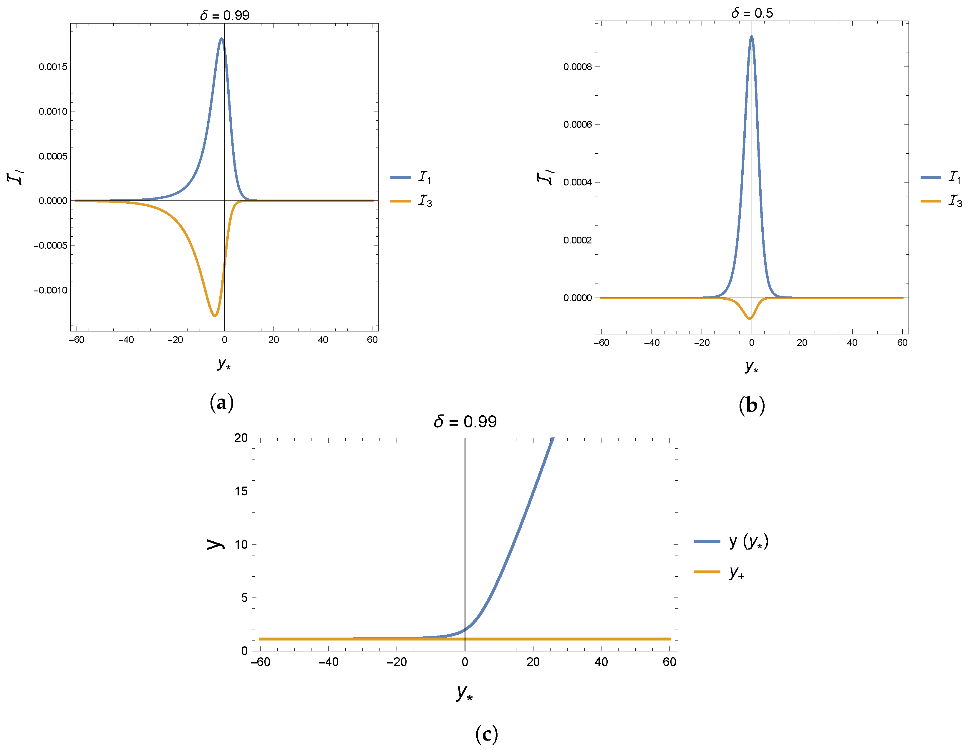
In our numerical analysis, we consider ; then, the relevant functions for us are and , shown in Figure 1 for two different values of . The maximal contribution occurs in the region , that is, toward the outer horizon, while contributions from are negligible.
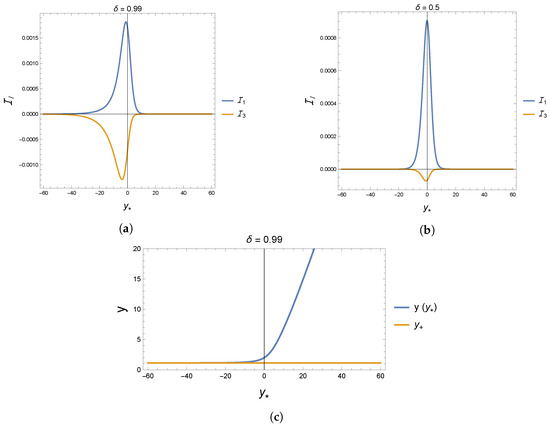
Figure 1.
Panels (a) and (b) show the function defined in (34) for two different black holes’ rotation velocity , for and . Panel (c) shows and the coincidence of (the horizon) with . (a) Function vs. rescaled tortoise coordinate for , (b) Function vs rescaled tortoise coordinate for , (c) The coordinate y as function of and the horizon .
In Figure 1c, we can check that, for , the horizon is reached at . Then, numerically, is a good approximation for the limits .
The source terms in (31) is, therefore, zero for even values of ℓ, while, for the two other cases under analysis, they are
with given in Appendix A, and
4.2. Numerical Solutions
The potential in the limits previously discussed has the following asymptotic behavior:
with . We can treat the equation as an homogeneous equation in these limits since the source can be taken to be zero there, as shown in Figure 1.
The asymptotic solutions are, therefore
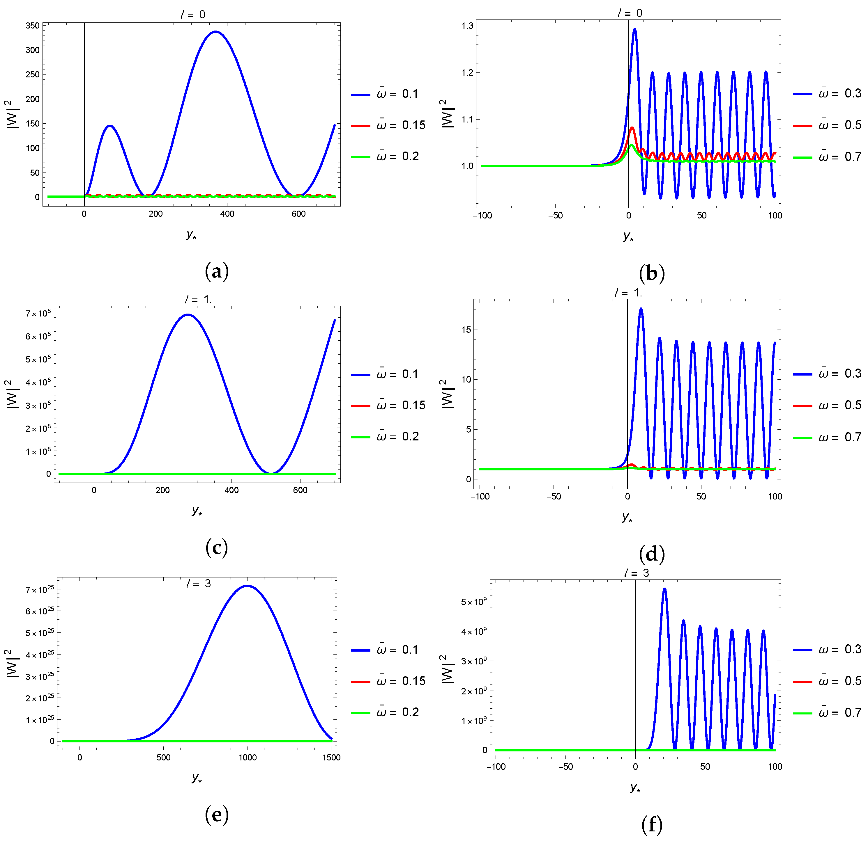
Following [14], we choose . Numerical solutions for this choice are displayed in Figure 2 for .
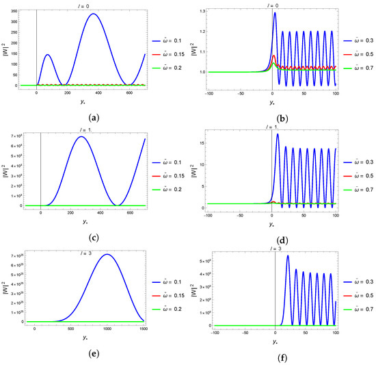
Figure 2.
The amplitude for , , and for different values of . (a) for and , (b) for and , (c) for and , (d) for and , (e) for , and , (f) for , and .
As we pointed out before, the source components are non-zero for odd ℓ (shown in Figure 1a,b). It is interesting to compare with the sourceless case.
In Figure 3, we plot the case and for different values of , comparing the solution with and without the source.
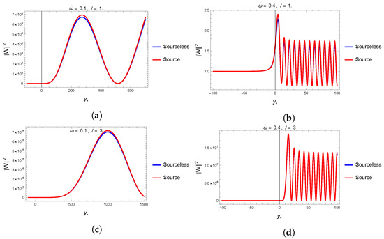
Figure 3.
The amplitude for , , and for the cases with and without source term. (a) for and . Effect of the source term. (b) for and . Effect of the source term. (c) for and . Effect of the source term. (d) for and . Effect of the source term.
The source mainly affects the maxima (peaks) of , but not the position of these peaks. Additionally, the amplitude increases for higher values of ℓ, and the highest amplitudes occur for . This last condition, , corresponds to the longwave approximation.
Indeed, Equation (22) is analogous to the partial wave method in quantum mechanics theory but with spheroidal harmonics instead of Legendre polynomials.
In (24), we can write , where is the momentum of the scalar field, and, therefore, the limit is equivalent to , which is the well-known long-wave approximation (LWA) introduced by Isaacson [29] in gravitational radiation. However, we emphasize, and we must not lose sight of this, that must be understood, of course, as .
In this approximation,
and .
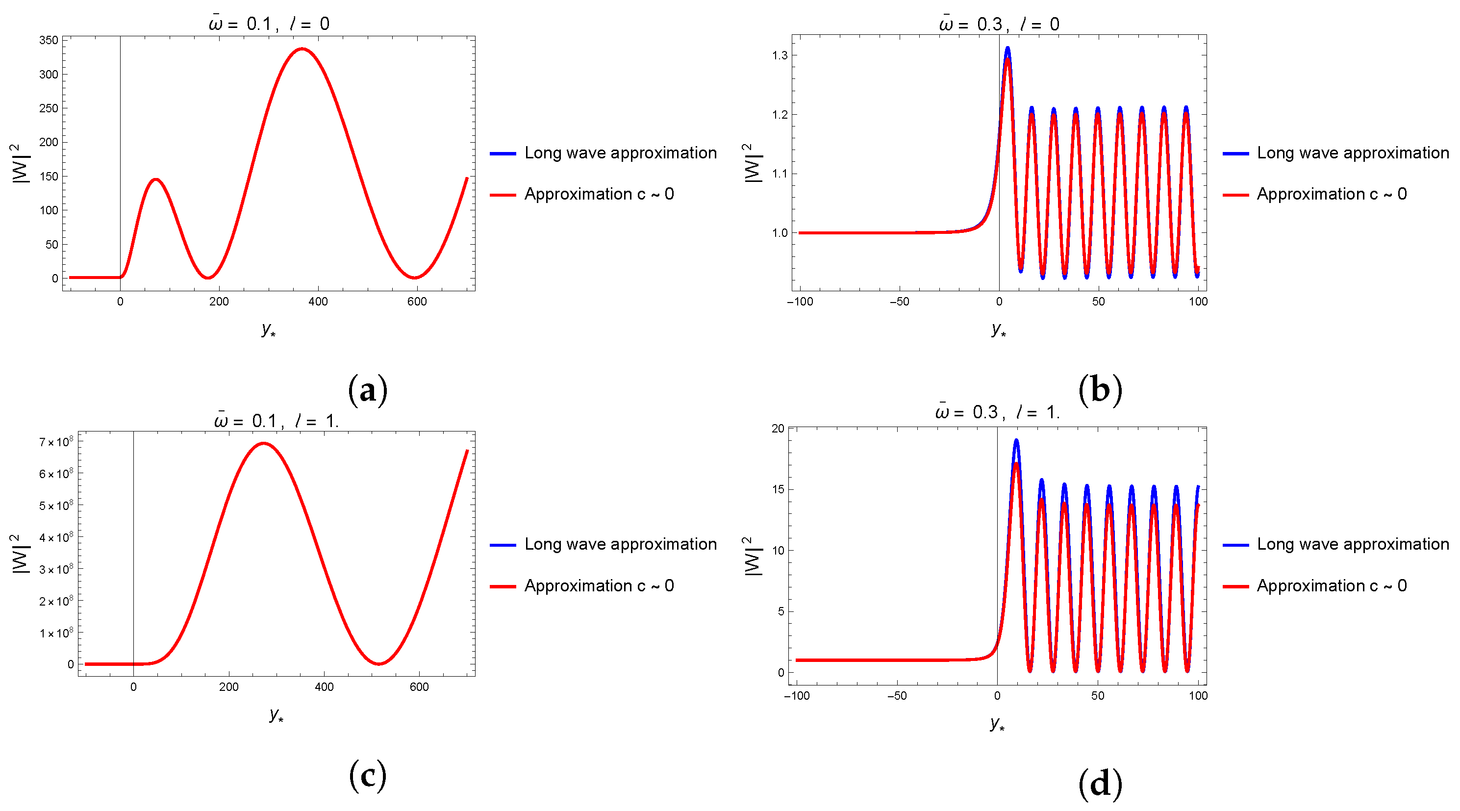
We can compare the solutions obtained by setting with those coming from the general treatment in the Appendix A. The results are shown in Figure 4.

Figure 4.
Compared amplitudes for , , and different ℓ. In one case, we use the long-wave approximation, while the other corresponds to the solution calculated with the perturbative approach described in the Appendix A. (a) obtained in the long-wave approximation compared with the approximated solution for and . (b) obtained in the long-wave approximation compared with the approximated solution for and . (c) obtained in the long-wave approximation compared with the approximated solution for and . (d) obtained in the long-wave approximation compared with the approximated solution for and .
The numerical solutions presented in Figure 1, Figure 2, Figure 3 and Figure 4 show that (a) the source considered in the present work is relevant in the region near the horizon, but, in the limit , the equation for the scalar field can be safely taken as (31) with the asymptotic form of the effective potential given in (41) and sourceless; (b) for numerical purposes, the choice is enough to guarantee that we are close enough to the horizon and infinity (depending on the sign of ); (c) the case can be treated using the long-wave approximation, or the expressions for obtained in the Appendix A.
In the following section, we discuss the radiation pattern of the solutions analyzed here.
5. Emission of Radiation
Following [14], the emission of axions’ radiation due to the source in (12), per unit frequency interval per solid angle , is
The angular term depends on but we omit this in the analysis since it represents a small contribution, as seen in the appendix, where this term is plotted as a function of the frequency.
Another interesting quantity to characterize the radiation emission is the fractional energy gain from the monochromatic wave sent from infinity. In our case, this quantity is
where is calculated in a similar way as :
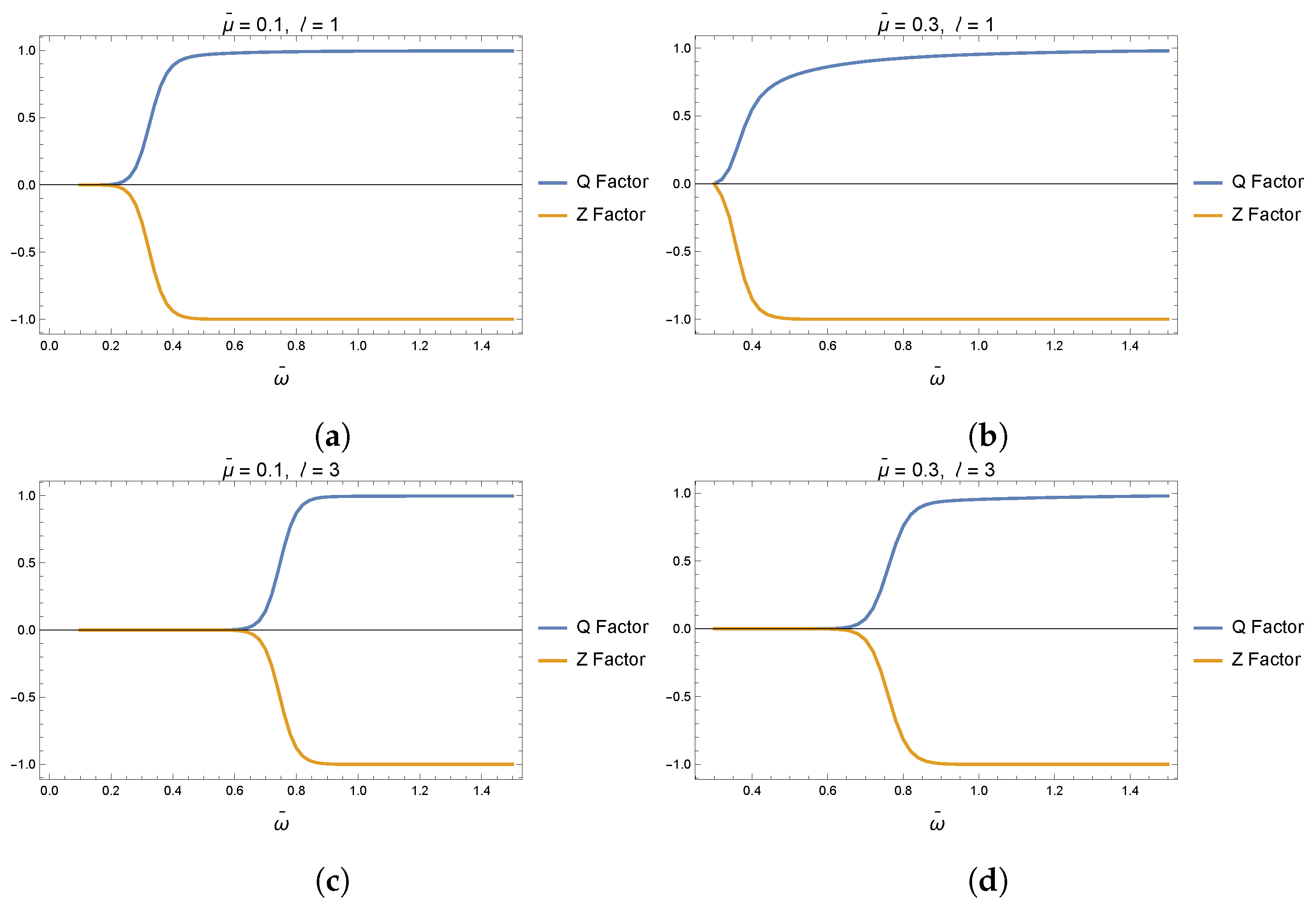
Figure 5 shows Q and Z for and . For the case (and for all even values of ℓ), the source term is zero; however, for even values of ℓ, the source is relevant. Figure 5c,d shows how different the factors Z and Q are when the source is considered.
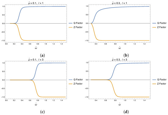
Figure 5.
Factors Q and Z defined in the text for different values of ℓ and . In all panels, . (a) Factors Q and Z for and . (b) Factors Q and Z for and . (c) Factors Q and Z for and . (d) Factors Q and Z for and .
With these results, we numerically calculate the total energy radiated to infinity up to the constant coming from the solid angle integration, that is,
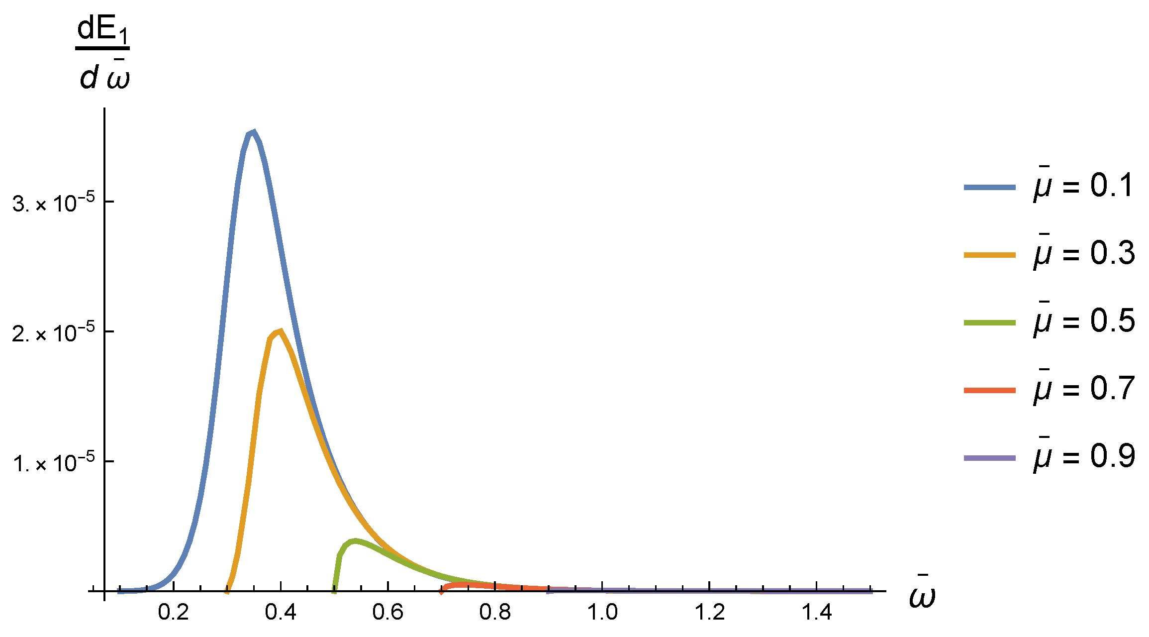
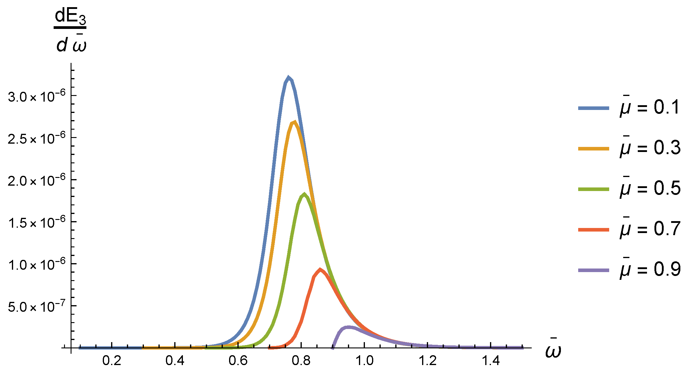
which is not zero only for odd values of ℓ. In our case, this is . The results are plotted in Figure 6.
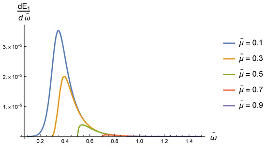
Figure 6.
Radiated energy as a function of for different masses and . Factors Q and Z for .
Let us comment on the results shown in this numerical analysis. According to Detweiler in [14], a sharp maximum in Q signals a resonant frequency at which a black hole resonance occurs. In our case, this resonance does not happen, as seen in Figure 5.
To understand this, first note that our initial condition (numerical integration condition) is near the horizon ( or, numerically, ). On the other hand, functions Z and Q start from zero at the initial frequency , then Z increases while Q decreases, which happens during a frequency interval, let us say . By denoting the half of such an interval as , the function Z behaves as follows:
and a similar expression for Q, changing the last line to 1.
From the definition of Q and Z, previous behavior is understood due to the following. For , the denominator in (46) produces a divergence that is responsible for . Instead, for Z, such divergence is not present since Z depends on the ratio (see the definition of in (48)) and then, for this frequency range, .
Instead, for , the conditions and are consistent with the behavior of the Z and Q factors.
The Z factor is the fractional energy gain of a wave of frequency sent from infinity that is scattered from the BH. In the zone where , part of the incoming wave is scattered (indeed, in this frequency range, , while, in the region in which , no scattered wave is present, indicating a complete absorption of the signal).
Therefore, the energy radiated should be centered in the transition zone, the region. Figure 6 and Figure 7 precisely show this behavior.
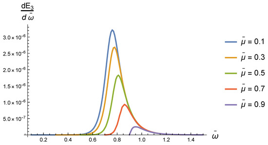
Figure 7.
Radiated energy as a function of for different masses and . Factors Q and Z for .
6. Conclusions
This research paper explores the movement of gravitational axions in a Kerr black hole background using analytical and numerical methods. One interesting finding is that resonance occurs when , similar to the Detweiler resonance discussed in [14]. However, the Detweiler resonance is related to a massless scalar. This research concludes that this resonance always occurs if ℓ is odd and a Pontryaguin-like source is present.
Another important observation is that Figure 6 and Figure 7 show that the spectral maxima shift to the right and the radiated power decreases with . Additionally, the maximum becomes significantly smaller when ℓ grows. However, it is interesting to note qualitatively that the curves can be reasonably approximated as Gaussian for small .
For , the Gaussian starts to be asymmetric with a deviation to the right. We found that the function
is well-fitted to the curves of the radiated power. Here, is the error function
The function f in (51) is proportional to the probability density of a skew-normal distribution, with proportionality constant a and, for this distribution, it is known that the mean value is
and the variance is
We summarizes these results in Table 1.

We estimate the mean lifetime of these resonances as (dimensionful quantities)
Then, for example, primordial black holes with their masses ranging from Planck mass () to masses of order will cause pulses with a mean lifetime from [s] up to [s] years, that is (in the last case), a mean lifetime well beyond the universe’s age.
It is worth noting that the resonance for gravitational axions discussed in this paper is distinct from the one studied in Detweiler’s work. In Detweiler’s case [14], the resonance is observed as a divergence of the factor , whereas, in our case, approaches 1 as tends to infinity.
In conclusion, observing sharp resonances in radiation patterns is possible, depending on the black holes’ mass. For instance, if the black holes have masses between 100 and 1000 , the lifetime of these resonances falls within the range of observability in LIGO [18].
Finally, it is important to point out that superradiance is a phenomenon that appears naturally in the homogeneous part of Equation (17), and it is for this reason that it is not relevant in the treatment of the Teukolsky equation.
Author Contributions
All authors (J.G. and F.M.) have equally contributed to the manuscript. All authors have read and agreed to the published version of the manuscript.
Funding
This research was funded by The Alexander von Humboldt Foundation(JG), and FONDECYT through the grants 1221463 (J.G.), and DICYT-USACH through the grant 042231MF (F.M.)
Data Availability Statement
No new data were created or analyzed in this study.
Acknowledgments
J.G. thanks Christophe Grojean for the pleasant hospitality in DESY (Hamburg); he also thanks Thomas Biekötter and Mathias Pierre for the pleasant discussions at the DESY lunch, and also mainly to Andreas Ringwald and Pierre Sikivie for sharing their knowledge of axions with him. We thank Manu Paranjape for clarifying discussions on subtle aspects of this paper.
Conflicts of Interest
The authors declare no conflict of interest.
Appendix A. The Angular Equation
In this appendix, we review the solution of (19) following the analysis by S. Teukolsky in [25]. First, define, as usual, , so that the angular equation is now
In reference [25], a method for treating the case of any spin s and third component of angular momentum, m, is discussed. However, we restrict here to the case of interest for us, that is, and , which is just the previous equation.
The idea is to treat the term as a perturbation (not necessarily infinitesimal). The order-zero operator is
with the known (normalized) solution
with (), and is the Legendre’s polynomial of degree ℓ.
The continuation method [30] for calculating eigenfunction and eigenvalues in (A1) considers c as a parameter, and then the equation under study is
with ′ denoting derivatives with respect to x and .
By taking the derivative with respect to c in the previous equation (denoted by a dot in what follows), one obtains
From here, it is possible to find a set of first-order differential equations for and . Indeed, multiplying the last equation by followed by an x integration, one obtains
The first term can be integrated by parts twice, giving (boundary terms cancel)
Then, the first and second terms cancel in (A6). Finally,
with .
We repeat the calculation, but multiplying now by with , and performing the integral to obtain
Finally, with the help of the completeness relation, one obtains
Equations (A8) and (A10) are a system of differential equations to be solved (numerically) to determine the eigenvalues and eigenfunctions in Equation (A1).
In this perturbative approach, the solution of the problem at zero order is given by (A3); then, we look for solutions of (A8) and (A10) with the form
which, once replaced in the equations, give rise to
with
Equations must be solved with the following initial conditions:
Expressions (A12) and (A13) are those in [25]. In Teukolsky’s approach, the normalization is assumed, specified in our case for the massive scalar field, and the third component of angular momentum equals zero.
The case can be treated similarly, and the only effect is a change of signs in the RHS of (A12) and (A13). However, this case is not interesting since it produces divergent solutions for .
Our analysis focuses on the cases . The numerical solutions are obtained by summing up to in (A11) and subsequent expressions. The solutions are fitted to a polynomial function, and we found that the best fit (for ) is obtained for order-five or higher polynomials.
The results for eigenvalues with are the following:
These coefficients are the non-zero ones, which are relevant to our approximation. For example,
and similar expressions for , with the coefficient listed before.
Finally, note that, for the radiation emission, the quantities of interest are , which, once integrated into the solid angle, will be 1. However, our approach has an explicit dependence on c:
Figure A1 shows that, even if there is such a dependence, these integrals can be approximated to 1 in our numerical analysis.
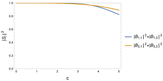
Figure A1.
Contribution of to the normalization of functions.
Figure A1.
Contribution of to the normalization of functions.

References
- Peccei, R.D.; Quinn, H.R. CP Conservation in the Presence of Instantons. Phys. Rev. Lett. 1977, 38, 1440–1443. [Google Scholar] [CrossRef]
- Weinberg, S. A New Light Boson? Phys. Rev. Lett. 1978, 40, 223–226. [Google Scholar] [CrossRef]
- Wilczek, F. Problem of Strong P and T Invariance in the Presence of Instantons. Phys. Rev. Lett. 1978, 40, 279–282. [Google Scholar] [CrossRef]
- Sikivie, P. Experimental Tests of the Invisible Axion. Phys. Rev. Lett. 1983, 51, 1415–1417, Erratum in Phys. Rev. Lett. 1984, 52, 695. [Google Scholar] [CrossRef]
- Kandus, A.; Kunze, K.E.; Tsagas, C.G. Primordial magnetogenesis. Phys. Rept. 2011, 505, 1–58. [Google Scholar] [CrossRef]
- Anzuini, F.; Maggi, A. Axions and primordial magnetogenesis: The role of initial axion inhomogeneities. J. Cosmol. Astropart. Phys. 2024, 8, 011. [Google Scholar] [CrossRef]
- Grasso, D.; Rubinstein, H.R. Magnetic fields in the early universe. Phys. Rept. 2001, 348, 163–266. [Google Scholar] [CrossRef]
- Soliman, N.H.; Hopkins, P.F.; Squire, J. Dust Battery: A Novel Mechanism for Seed Magnetic Field Generation in the Early Universe. arXiv 2024, arXiv:2410.21461. [Google Scholar]
- Domcke, V.; Ema, Y.; Mukaida, K. Chiral Anomaly, Schwinger Effect, Euler-Heisenberg Lagrangian, and application to axion inflation. J. High Energy Phys. 2020, 2, 55. [Google Scholar] [CrossRef]
- Jackiw, R.; Pi, S.Y. Chern-Simons modification of general relativity. Phys. Rev. D 2003, 68, 104012. [Google Scholar] [CrossRef]
- Alvarez-Gaume, L.; Witten, E. Gravitational Anomalies. Nucl. Phys. B 1984, 234, 269. [Google Scholar] [CrossRef]
- Adler, S.L. Axial vector vertex in spinor electrodynamics. Phys. Rev. 1969, 177, 2426–2438. [Google Scholar] [CrossRef]
- Bell, J.S.; Jackiw, R. A PCAC puzzle: π0→γγ in the σ model. Nuovo Cim. A 1969, 60, 47–61. [Google Scholar] [CrossRef]
- Detweiler, S.L. Resonant oscillations of a rapidly rotating black hole. Proc. Roy. Soc. Lond. A 1977, 352, 381–395. [Google Scholar]
- Press, W.H.; Teukolsky, S.A. Floating Orbits, Superradiant Scattering and the Black-hole Bomb. Nature 1972, 238, 211–212. [Google Scholar] [CrossRef]
- Damour, T.; Deruelle, N.; Ruffini, R. On quantum resonances in stationary geometries. Lett. Nuovo Cim. 1976, 15, 257–262. [Google Scholar] [CrossRef]
- Dolan, S.R. Instability of the massive Klein-Gordon field on the Kerr spacetime. Phys. Rev. D 2007, 76, 084001. [Google Scholar] [CrossRef]
- Jung, S.; Kim, T.; Soda, J.; Urakawa, Y. Constraining the gravitational coupling of axion dark matter at LIGO. Phys. Rev. D 2020, 102, 055013. [Google Scholar] [CrossRef]
- Fujita, T.; Obata, I.; Tanaka, T.; Yamada, K. Resonant gravitational waves in dynamical Chern-Simons-axion gravity. Class. Quant. Grav. 2021, 38, 045010. [Google Scholar] [CrossRef]
- Myung, Y.S. Superradiant instability of a massive scalar on the Kerr spacetime. arXiv 2022, arXiv:2206.14953. [Google Scholar]
- Detweiler, S.L. Equations governing electromagnetic perturbations of the Kerr black-hole. Proc. Roy. Soc. Lond. A 1976, 349, 217–230. [Google Scholar]
- Alexander, S.; Yunes, N. Chern-Simons Modified General Relativity. Phys. Rept. 2009, 480, 1–55. [Google Scholar] [CrossRef]
- Eguchi, T.; Gilkey, P.B.; Hanson, A.J. Gravitation, Gauge Theories and Differential Geometry. Phys. Rept. 1980, 66, 213. [Google Scholar] [CrossRef]
- Deriglazov, A.A.; Ramírez, W.G. Ultrarelativistic Spinning Particle and a Rotating Body in External Fields. Adv. High Energy Phys. 2016, 2016, 1376016. [Google Scholar]
- Teukolsky, S.A. Perturbations of a rotating black hole. 1. Fundamental equations for gravitational electromagnetic and neutrino field perturbations. Astrophys. J. 1973, 185, 635–647. [Google Scholar] [CrossRef]
- Abramowitz, M.; Stegun, I.A. Handbook of Mathematical Functions with Formulas, Graphs, and Mathematical Tables; Dover Publications: New York, NY, USA, 1965. [Google Scholar]
- Breuer, R.A.; Ryan, M.P.; Waller, S. Some properties of spin-weighted spheroidal harmonics. Proc Roy. Soc. 1977, 358, 71. [Google Scholar]
- Flammer, C. Spheroidal Wave Functions; Dover Publications: Mineola, NY, USA, 2014. [Google Scholar]
- Isaacson, R.A. Gravitational Radiation in the Limit of High Frequency. I. The Linear Approximation and Geometrical Optics. Phys. Rev. 1968, 166, 1263–1271. [Google Scholar] [CrossRef]
- Wasserstrom, E. A new method for solving eigenvalue problems. J. Comp. Phys. 1972, 9, 53. [Google Scholar] [CrossRef]

Disclaimer/Publisher’s Note: The statements, opinions and data contained in all publications are solely those of the individual author(s) and contributor(s) and not of MDPI and/or the editor(s). MDPI and/or the editor(s) disclaim responsibility for any injury to people or property resulting from any ideas, methods, instructions or products referred to in the content. |
© 2024 by the authors. Licensee MDPI, Basel, Switzerland. This article is an open access article distributed under the terms and conditions of the Creative Commons Attribution (CC BY) license (https://creativecommons.org/licenses/by/4.0/).