Abstract
Energy efficiency and consumers’ role in the energy system are among the strategic research topics in power systems these days. Smart grids (SG) and, specifically, microgrids, are key tools for these purposes. This paper presents a three-stage strategy for energy management in a prosumer nanogrid. Firstly, energy monitoring is performed and time-space compression is applied as a tool for forecasting energy resources and power quality (PQ) indices; secondly, demand is managed, taking advantage of smart appliances (SA) to reduce the electricity bill; finally, energy storage systems (ESS) are also managed to better match the forecasted generation of each prosumer. Results show how these strategies can be coordinated to contribute to energy management in the prosumer nanogrid. A simulation test is included, which proves how effectively the prosumers’ power converters track the power setpoints obtained from the proposed strategy.
1. Introduction
The reinforcement of consumers’ role in energy systems and the improvement of energy efficiency, in general, are among the key actions established in the European Strategic Energy Technology (SET) Plan [1]. This paper deals with some of the main topics in this SET Plan—energy monitoring and forecasting, consumers’ role in demand response (DR), and energy production and storage management—to achieve a higher renewable energy penetration and to improve energy efficiency. It is focused on a prosumer nanogrid [2], where prosumers have generation and energy storage systems (ESS) and they have control over their demand. Many studies about each of those topics can be found in the recent scientific literature. However, the combination of them in a whole management strategy has been hardly addressed in other works.
Wide attention has been paid to energy management systems (EMS) in microgrids, which may be applied to small-scale nanogrids, although they are not usually focused on prosumer-based microgrids. Literature on microgrids EMS is usually focused on defining the objective function to optimize the economic benefit within the microgrid [3,4]. Energy trading among different agents, like microgrids [5,6] or prosumers [7], has also been studied, with the aim of defining an incentive scheme for energy trading. However, none of these works provide a joint perspective of energy monitoring and forecasting, DR, and storage management, which is the main contribution of this proposal. All these aspects are essential to move towards Renewable Energy Communities, encouraged by the European Union in Directive (EU) 2018/2001 [8].
Mass digitization and the Internet of Things (IoT) are transforming many industries (Industry 4.0) and residential zones. This implies that the latest advances related to communication technologies, monitoring devices, and multiple data processing algorithms constitute qualitative progress that makes it possible to introduce more monitoring points as part of the Advanced Metering Infrastructure (AMI) [9] in the SG at all voltage levels [10,11].
The methods for permanent monitoring of power quality (PQ) and reliability analysis have to be adapted to large-scale deployments and campaigns, where time and space compression plays a special role. For this reason, the market for industrial and manufacturing PQ equipment is growing significantly, and consequently, several areas of knowledge are converging and pushing it up (e.g., Statistical Signal Processing and Instrumentation). In fact, while traditional PQ instruments have been devoted to developing specific measurement campaigns with the goal of capturing certain types of events, the current electrical network demands a flexible strategy capable of measuring new types of PQ disturbances as a result of non-optimized managements. Consequently, the number of fixed PQ analyzers has increased, and massive data are managed according to different measurement strategies, depending on the European country [12]. The SG demands an enhanced role for individual customers and prosumers taking part in the decisions in a new market model [13], where new energy profiles are appearing [14] and learning-based systems help empower customers to select companies according to the price and electricity fulfillment [15]. In this sense, it is crucial to fill in the gap between the energy delivered by utilities, and how end users assess its quality. According to the current nanogrid framework, it would be desirable to monitor the energy delivery and the PQ in the point of common coupling (PCC) and within the prosumers’ sides. In addition, weather and energy should be forecasted to guarantee that the smart appliances (SA) operate properly.
Popularly, SA are recognized for having some modern computer-based communication technology to make their tasks faster, cheaper, or more energy efficient. For example, smart washing machines can independently regulate the washing powder and the detergent to be used depending on the weight of the load and the type of fabric. They can also automatically send alerts when the detergent runs out. However, in the energy field, within the framework of SG, the term “smart” refers to those appliances capable of modulating their electricity demand in response to signal request from the electrical system [16,17,18]. Thus, household appliances could incorporate different DR strategies.
Generally, DR policies can be divided into direct (explicit DR) through aggregation, or indirect (implicit DR). Explicit DR (also called incentive-based DR program) is divided into traditional (e.g., direct load control—DLC, interruptible pricing) and market-based (e.g., emergency DR programs, capacity programs, demand bidding programs, and ancillary services market programs). On the other hand, implicit DR (sometimes called price-based DR programs) refers to the voluntary program in which consumers are exposed to electricity prices that vary over time, for example, time-of-use prices, prices at critical peaks, and real-time prices. For appliances, this would take the form of load-shifting strategies, which change their period of operation from peak to non-peak hours, or load-modulating strategies, which directly reduce or avoid energy use during peak hours [19].
EMS requires flexibility to match demanded energy with generated energy. As well as DR techniques, ESS definitely contribute to such flexibility. In microgrids, ESS usually have functions related to peak shaving and mitigation of intermittent generation fluctuation, typical of some renewable energy sources, like photovoltaic (PV) [20]. ESS management also aims to obtain economic advantages in literature [3,4]. In this paper, the role of ESS focuses on collaborating with DR techniques to outperform the management capability of the nanogrid energy.
Figure 1 depicts a scheme of the different stages of the proposed strategy. The first stage constitutes a forecasting tool, which can be used to estimate the PV generation power profile, as well as the weather variables, which influence energy consumption; the second stage performs a DR technique to optimize the consumption power profile; finally, the first stage schedules the ESS power profile with the aim of reducing the nanogrid dependence on the main grid. A simulation of the prosumer-based nanogrid is then carried out to test the results.
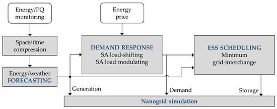
Figure 1.
Scheme of the stages of the proposed energy management system for the nanogrid.
This paper is organized as follows: Section 2 is focused on energy monitoring and forecasting; a DR method based on SA is proposed in Section 3; Section 4 is devoted to optimizing the ESS scheduling within the nanogrid; Section 5 presents a simulation test of power converters control to track obtained power setpoints; Finally, Section 6 summarizes conclusions.
2. Nanogrid Energy Monitoring and PQ Forecasting
Some recent works on the role played by forecasting in demand and storage management are related to managing uncertainties from renewable generation, electric load demand, temperature, and PV energy storage. Different energy demand strategies are proposed from the demand side and the generation side based on operating and environmental costs. Operational optimization of hybrid renewable energy systems (HRES), such as solar, wind, and diesel generation as backup resources and battery storage, helps manage system sizing in a local framework [21]. Additionally, coordinating virtual ESS using electric vehicles as more flexible resources, introducing intra-hour adjustment stage. The objectives are to adjust the different forecasting errors and to monitor the response characteristics based on scenarios [21,22].
Indeed, optimal economical dispatch plays an important role in order to minimize the microgrid operating costs and reduce the energy costs compared with different strategies [21,23]. Hierarchical control structure and alternative forecasting techniques are implemented using autoregressive integrated moving average (ARIMA), exponential smoothing, and neural networks [24]. Some other optimal EMS incorporate the stochastic approach for microgrids using optimization algorithms of mixed-integrated linear programming (MILP), and GAMS (general algebraic modeling system) implementation using power optimization at minimum operational costs.
Along with this, weather forecasting strategies are needed in order to update the energy models to the local conditions and improve energy dispatch, taking advantage of all the energy resources. The introduction of weather forecasting models in predictive control [21,24] allows forecasting studies in a smaller scale (e.g., single residential buildings and tertiary buildings).
Nevertheless, none of these previous strategies introduces the power quality issues on the nanogrid energy forecasting management. This section points to space and time compression as the main forecasting solutions to manage data within the frame of an instrumental technique, which is, at the same time, extensive to all PQ disturbance types and applicable downstream and upstream of a nanogrid energy forecasting system. In addition, an easy-to-implement PQ index is proposed which is intended for prosumers and house-hold appliances (Figure 2).
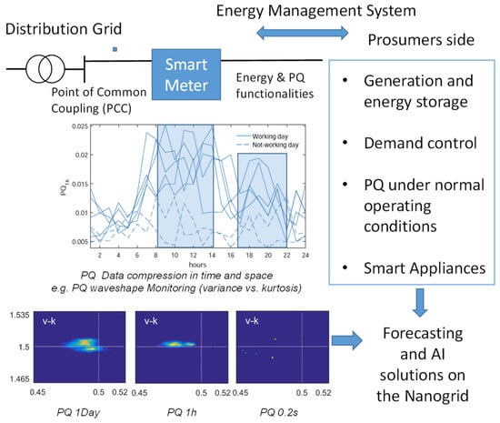
Figure 2.
Energy and power quality (PQ) monitoring strategy, previous step to forecasting and artificial intelligence (AI) on the nanogrid [25].
The reporting levels along with the allocations within the entire network are usually interpreted through the PQ triangle [9], in which time and space compression are concepts of high importance when monitoring PQ. Time compression implies reducing one time-series to a number and usually converts one unit (e.g., Volts) into another different unit (e.g., root mean square - RMS). Space compression consists of the reduction of the same measurement taken from several locations at the same level (e.g., site index) with the goal of characterizing an area (e.g., feeder index) within a microgrid, or a prosumer in a nanogrid. The proposed method for massive data acquisition and representation may consist of scheduled data acquisition and processing data and can be applied on a nanogrid. Given a time window of length Δt, the M time-series of measurements are compressed in the time domain, as each N-point register is reduced to a single data point in the 2D space. The statistic versus statistic representation allows a better understanding of the system’s dynamic, as the evolution of the vector indicates the energy fluctuation. Depending on the total elapsed time (multiple of Δt), the trajectory accounts for PQ or reliability operation.
The proposed unified PQ index is calculated via (1), in which the averaged differences among the measurements sij and the ideal values (associated with a healthy power-line signal) of the statistics are computed.
The role of this index consists of monitoring the energy state within transactions between the actors in the system under normal operating conditions, i.e., the role of the monitoring system is to check if contractual conditions are fulfilled (e.g., frequency, voltage levels) to guarantee an adequate power supply that outperforms the management capability of the nanogrid. This strategy is an approximation to match PQ and energy forecasting data so as to enable adequate supply, i.e., to perform a forecast when the energy can be supplied or when the supply is most convenient (Figure 2). Hereinafter, we show the performance of real-life instrumental examples within a week measurement campaign.
3. Demand Response by Means of Smart Appliances
In order to test the effectiveness of the most common DR techniques, a control platform composed of four blocks has been proposed, that collects and exchanges information, aiming to minimize the demand peaks and, therefore, to reduce the electricity bill by means of the DLC. Figure 3 refers to the architecture of the proposed platform, in which the core application developed with LabVIEW is in charge of processing the data provided by the rest of subsystems.
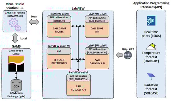
Figure 3.
Block diagram of the proposed smart appliances control platform, including the GAMS (general algebraic modeling system) engine and middleware in charge of linking it to LabVIEW, the application core and Application Programming Interfaces (APIs) that provide the data.
To achieve the abovementioned goal, DR policies will be implemented through an optimization model, specifically an MILP model that includes in its constraints details such as the SA nature, the people’s behavior, and the amount of available energy that could be imported from the main sources taken into account. As can also be depicted from Figure 3, the optimization engine of GAMS was used due to its flexibility, as it makes it possible to state the mathematical formulation without regarding the number of decision variables, and also a straightforward way of interaction from many environments. A middleware written in C++ which internally uses the object-oriented Application Programming Interface (API) that the company provides for interacting purposes makes possible the link with the application core. In this sense, the MILP model that will be raised in the following lines can be solved simply by calling this middleware with the appropriate parameters. The block on the right of Figure 3 is related to the APIs that furnish the data to the optimization model (real-time prices—RTP, temperature and radiation forecast), therefore, three LabVIEW subVIs have been dedicated for managing the communication between them via HTTP.
Concerning the model, this paper proposes a novel MILP to optimize the cost of the daily household energy consumption and thus ensure the peak demand minimization using a strategy based on the DLC. Equation (2) refers the objective function f (in €) and the daily cost of the energy, where Pgrid(t) (in kW), RTP(t) (in €/kWh) and Δt (in hours) are the power imported from the utility, the hourly price of the energy at time slot t ∈ [1, …T], and the time resolution given by , being T equal to 24 h. This means a resolution of 1 h, which is more than enough for the platform, as it is devised to work in the highest control layer of the nanogrid (tertiary control).
The rest of the equations are related to the power balance and user preferences and have been expressed as constraints within the model. Equation (3) refers to the power balance at each time slot , being the foregoing power Pgrid(t) and the PV production Ppv(t) (in kW) on the generation side. On the demand side is the non-shiftable power Pns(t) (in kW), coming from uncontrollable loads such as lighting and small devices or simply the standby consumption. Pwm(t), Pdw(t), and Ptd(t) (in kW) are also on this side and represent the power consumption of the well-known SAs that can be found within a residential environment, in particular, the washing machine (WM), the dishwasher (DW), and the tumble drier (TD) respectively, the averaged consumption of the water heater (WH) has been expressed by Pwh(t) (in kW). Equation (4) establishes the upper limit of the power taken from the grid by means of , which represents this value.
The previous power demands of each SA are expressed in Equations (5)–(7) through their averaged consumption profiles Dwm, Ddw, and Dtd (in kW), which are vectors with T components: the first two represent the averaged consumption and the rest of them are zero, since the time cycle of these SAs has been chosen to be 2 h. The employed strategy entailed building as many rotated demand profiles as the vectors DVwm, DVdw, and DVtd indicate for each SA, where each one of their components DVwm(i), DVdw(j), and DVtd(k), denote the number of slots that the original demand profiles Dwm, Ddw, and Dtd must be rotated to the right to generate a new possibility (in this case, one slot matches one hour, since T = 24). The number of rotated profiles is denoted by dwm, ddw, and dtd, respectively, for each SA. Furthermore, these rotated demands have also been associated with each component Swm(i), Sdw(j), and Std(k) of the binary decision vectors Swm, Sdw, and Std, which represent their states: when the model is solved, these variables may be 1 or 0 and thus this rotated demand will be the final scheduled demand or not. Equation (8) forces the number of binary variables of each decision vector that are equal to 1 and thus the number of cycles.
Equation (9) describes the WH dynamic and regards its thermal inertia as well as parameters such as the instantaneous energy flow with the environment, , and the energy supplied by the inlet water, and the heating element, , for each time slot t. Parameters such as ρ (in kg/m3) and Cp (in J/kg∙K) model essential supply water characteristics like its density and specific heat, while Tinlet refers to its average temperature, which is typically computed over a one-month time horizon. The WH design and dynamic also influence the tank capacity and the loss factor Cwh (in m3) and gwh (in W/K), respectively. Twh(t) and Twh(t − 1) (in K) are the current and the last value of the water temperature inside the tank. Finally, the user assumes an active role again by selecting the hourly water demand Dwt(t) (in m3) and the temperature limits in Equation (10), where the vector represents the minimum temperature of the water for each hour and the maximum admissible temperature, both in K. Starting from the user selection, the vector is generated according to Dw(t): if the water demand in t is zero, the minimum temperature matches the Tinlet, otherwise, the minimum temperature is set to the temperature selected by the user.
where:
Under this framework, a case of study of a typical dwelling found in residential environments with a PV system of 2 kW and maximum power,, of 3.6 kW located in Cordoba (Spain) was chosen according to the platform scheme followed. The WH parameters were selected according to specifications that commercial electric water heaters provide for the selected capacity (Cwh = 150 L): and set at 65 °C and 90 °C, respectively, and gwh equal to the standard value 15 W/K. The inlet water temperature, Tinlet, depends on the month of the year and the worst case (6 °C) suggested by the report [26] was selected. Besides these parameters previously fixed, Figure 4a–c shows the demand profiles selected that model the consumption of the common-use SA [27] to obtain 1 h resolution power profiles to be used by LabVIEW. Furthermore, the daily hot water demand (see the purple line in Figure 4d) used in this case study was based on [28], which considers the household usage (i.e., showering, cooking, or dishwashing). The non-shiftable power (red demand of Figure 4d) was obtained by monitoring the active power for a 24-h workday in one of the laboratory circuits. Subsequently, this profile was adapted to be used with the LabVIEW platform, which works with 1-h intervals, by computing the average. A scenario was assumed in which the user scheduled multiple SAs during the day under study, using a tariff with no hourly discrimination.
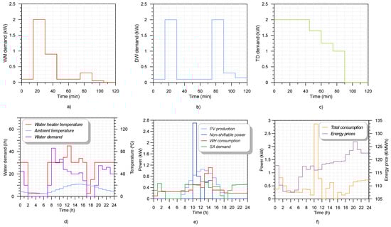
Figure 4.
(a–c) Smart appliances power demands; (d) hot water demand, ambient temperature, and water heater (WH) temperature once the model is solved; (e) photovoltaic (PV) production, non-shiftable power, WH demand, and decoupled demand of the SA; and (f) total demand consumption and real time prices.
Three SAs were scheduled with only one cycle of operation in this case example showing a 24-h pattern. Specifically, the WM was scheduled within the period 8:00–18:00, TD within 10:00–22:00, and DW to be launched at 13:00 h, which was added to the non-shiftable power described above. With respect to the results, note the relationship between the PV production and the water heater consumption from Figure 4d: at 12:00, the highest power consumption (around 0.6 kW) and the highest generation (around 1.1 kW) took place, showing the strategy followed by the WH, which consisted of increasing the temperature to store energy in high generation periods to be used at peak demand hours, and thus avoid more expensive energy hours due to its thermal inertia. Its temperature, shown in Figure 4d, also reached almost the maximum allowed at this time slot, which supports this operation principle. Clearly, Figure 4e shows the SA isolated demand and thus the hours allocated for them, which were the period 10:00–12:00 h for both the WM and the TD, since this time interval entails the highest power consumption of the day, approximately 2.8 kW, and satisfies the user preferences and the DW, which was scheduled in fixed mode, started its operation at 13:00. Through this case, it can be inferred that the platform considers it more suitable to use the available PV production as a more optimum power source than that provided by the grid, even in the cheapest energy hours. Finally, Figure 4f shows the daily profiles of the real-time prices (tariff with no hourly discrimination), and the power taken from the grid (still without ESS) from which the objective function was computed.
4. Cooperative Storage Management within the Prosumer Nanogrid
The households whose demands are managed are integrated within a nanogrid, which is composed of two neighbor households, among whose loads there are SAs which are managed as in Section 3. The same PV installation and production are assumed for both prosumers and each of them also has battery ESS with a capacity of 6 kWh and a maximum charging/discharging power of ±2 kW (Figure 5). Generation and initial demand hourly active power of each prosumer are shown in Figure 6a,b. It can be observed that the initial demand of prosumer 1 is the result of demand management performed in the case study of Section 3. A different demand profile is assumed for prosumer 2 to illustrate the storage management. In this final stage of nanogrid energy management, the energy interchange with the main grid is aimed to be minimized. Therefore, the schedule of charging/discharging power of both batteries is performed with this target.
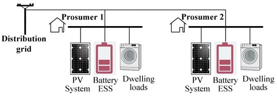
Figure 5.
Schematic of the demand and energy resources of each prosumer in the nanogrid under study.
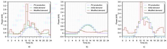
Figure 6.
Profiles of generation, initial demand, and modified demand for: (a) prosumer 1 individual scheduling; (b) prosumer 2 individual scheduling; and (c) global (prosumer 1 + prosumer 2) coordinated scheduling.
Generation and initial demand hourly power values are collected in 24-element vectors Ppv(t) and PD(t), respectively, with t = 1, 2, …, 24 h. PD vector equals the left part of Equation (3). A new 24-element vector PBi(t) is defined to collect the scheduled battery hourly power. When individual scheduling is performed, Ppv(t), PD(t) and PBi(t) correspond to each prosumer. However, if a coordinated operation is performed, Ppv(t) and PD(t) are the sum of prosumers’ generation and demand, and PB(t) is composed of 48 elements, i.e., two strings of the 24-hourly power values of each of the batteries, PBi(t). Elements of PBi(t) are the variables to be obtained as a result of the optimization process proposed. Once it has been obtained, a modified demand vector PDmod(t) is calculated with (11). Adopted sign criterion for PBi(t) is positive values when charging and negative values when discharging. Under this criterion, battery power behaves as demanded power, and it can be added to the consumers’ initial demand to obtain the modified demand, which better matches the generation profile.
The optimization process tries to find proper values for every PBi(t) vector with the aim of optimizing the balance between generation and modified demand, i.e., minimizing the power in the connection point with the distribution grid at every hour [29]. This target is directly related to the concept of energy autarky, because it aims to maximize both self-consumption (SC) and self-sufficiency (SS) of the nanogrid, thus optimizing the exploitation of the distributed energy resources. The objective function is shown in Equation (12).
Economic profits are usually the preferred objective function in grid-connected microgrid energy management [3,4]. However, when network tariffs are considered and self-consumption aids are not granted, the proposed objective function presents economic advantages as well as technical ones, as discussed in [30].
The optimization problem is also subjected to several constraints (further explanation in [29]): (i) The state of charge (SoC) of batteries must be kept within a safe operational range. In this work (20%, 100%) was assumed for this range; (ii) The discharging/charging power must not exceed the rated power of the battery’s power converter. In this work, maximum discharging and charging power rates were −2 and 2 kW; (iii) With the aim of smoothing batteries’ SoC variations, a maximum power gradient of 0.3 kW between consecutive hours was established.
Genetic algorithms (GA) were chosen to search for a proper solution for the optimization process. Although GA are not formally classified as optimization techniques, they have been widely used for energy management purposes, due to their ability to find a global solution even in non-convex, non-linear, and non-smooth optimization problems, and with either positive or negative values for the variables [29]. Both individual and cooperative operations were performed, to illustrate the advantages of energy sharing in the context of microgrids. The optimization results are depicted in Figure 6, where modified demand, once battery power was added to initial demand, is shown together with the initial demand and generation. It can be observed that both in individual and in a coordinated operation, modified demand better matches the generation profile, thus reducing the remaining power, which must be interchanged with the main grid at each hour.
Table 1 quantifies the results in terms of SC and SS (13) indices and absolute values of daily imported (Eimp) and exported (Eexp) energy. It can be observed that SC and SS indices increase due to the action of batteries in both individual and cooperative operation. In the case of total energy interchange with the main grid, cooperative scheduling of batteries clearly outperforms the situation without batteries as well as their individual operation.

Table 1.
Self-consumption (SC) and self-sufficiency (SS) indices and imported and exported energy as a result of batteries management.
5. Simulation of the Nanogrid
A nanogrid with two prosumers was simulated with Matlab/Simulink® to validate the performance of the proposed strategy in each prosumer’s power converters. The topology of the system was the same in both prosumers and it is depicted in Figure 7. The electric circuit in Figure 7 was modeled using Simulink/Power System Blockset. Switching devices of power converters were insulated gate bipolar transistors (IGBT)/diode pairs controlled by firing pulses produced by a Pulse Width Modulation (PWM) generator. Filters were built with passive elements and consumer load was a constant RL shunt impedance. A lead-acid battery model from the Power System Blockset modeled the storage device.
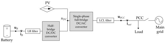
Figure 7.
Circuit scheme of each prosumer’s system, including PV generation, battery based energy storage systems (ESS), power converters and load.
The PV installation was assumed to be a current source, tracking its maximum power point (MPP). Two control loops were defined and programmed in the simulation model (by means of Simulink basic blocks and math operations): one for the battery current (which controls the DC/DC converter) and another one for the inverter output current (which generates the switching signals for the DC/AC converter). Both prosumers were connected to each other at the point of common coupling (PCC) bus.
The battery current reference was obtained from the algorithm of Figure 8. A proportional-integral (PI) controller, with constants KP = 0.4 and KI = 0.008, obtained the first term of the reference current, starting from the error between measured and reference values of the DC-link voltage (tuning guidelines for PI controllers can be found in [31]). Afterwards, once the system was connected to the grid, a second term, obtained from the planned power and the measured voltage of the battery, was added.
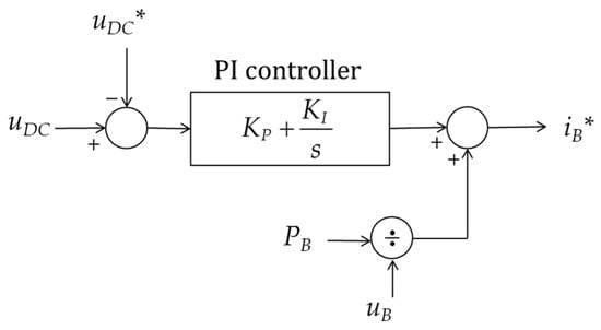
Figure 8.
Algorithm to obtain the battery current reference.
In this figure, uDC and uDC* are measured and reference values for the DC-link voltage, respectively; PB is the planned power for the battery, obtained from the optimization process described in Section 4; uB is the measured voltage of the battery; iB* is the resulting reference current; and KP and KI are the PI controller constants.
A dead-beat controller was used to obtain the duty cycle for the DC/DC converter that connected the battery to the other elements, as shown in (14) [32]. Switching signals for the converter gates were obtained from this duty cycle by means of a pulse width modulation (PWM) technique.
where dB is the duty cycle for the converter; iB is the measured value of battery current; RB and LB are the resistance and inductance of the filter (RB = 0.3 Ω, LB = 8 mH); and Ts is the sampling period (Ts = 1 × 10⁻⁴ s).
As was previously mentioned, the second control loop tried to track a reference in the output AC current of the inverter.
The reference current iout* was obtained in this paper from the single-phase PQ theory in the αβ reference frame [33]:
where P* is the active power output setpoint for the inverter (P* = Ppv − PB), Q* is the reactive power output (Q* = 0) and uPCCα and uPCCβ are the αβ components of the measured voltage in the PCC, uPCC, obtained by means of a Second Order Generalized Integrator—Phase-Locked Loop (SOGI-PLL) [33].
Once the reference current was calculated, a proportional-resonant (PR) controller was used to obtain the modulation signal for the inverter, as shown in Figure 9. This kind of controller is usually used in current controllers when a conversion from αβ to dq stationary frame is not required and, therefore, can be avoided [33]. The modulation signal enabled the switching signals for the gates in the DC/AC converter by means of a sinusoidal pulse width modulation (SPWM) technique.
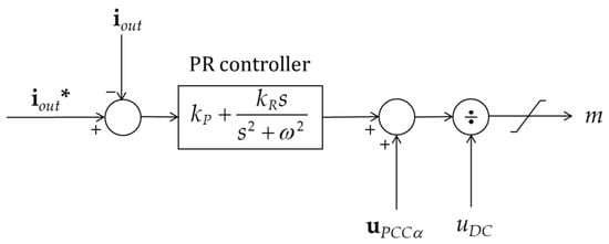
Figure 9.
Inverter output current control algorithm.
In this figure, iout is the measured output current, and kP and kR (20 and 2000 are the respective values, tuning guidelines for PR controllers can be found in [34]) are the controller constants.
The system was started and connected to the grid, according to the following event sequence: firstly, the battery adjusted the DC-link voltage up to a reference value of 400 V; secondly, the nanogrid was connected to the main grid; finally, the current controller for the DC/AC converter was activated, the PV installation connected, and the reference current for the battery was updated, starting from the planned battery power. Power values assumed for the test were those corresponding to the coordinated scheduling during period 13–14 h (Figure 6c), and they are detailed in Table 2.
Table 2.
Power values for each prosumer for the simulation test.
Figure 10 and Figure 11 show the simulation results. In Figure 10, the output current of both prosumers’ converters is depicted, along with the voltage signal in PCC (this one has been scaled for better visibility). Sinusoidal currents in phase with voltage were obtained in both cases. On the other hand, Figure 11 shows how, after a short transient period since control was activated, the active power output of each converter properly tracked the desired setpoints with a stable behavior.
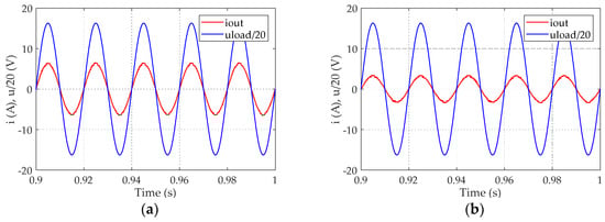
Figure 10.
Output current and point of common coupling (PCC) voltage signals for: (a) prosumer 1; (b) prosumer 2.
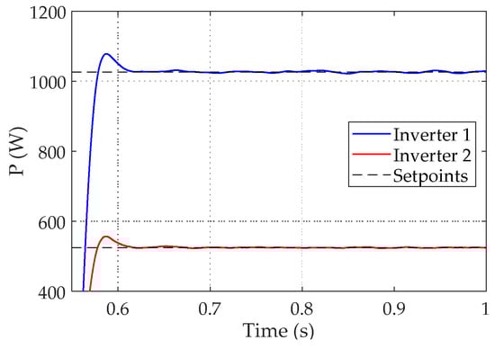
Figure 11.
Output power for both prosumers.
6. Conclusions
In this paper, an EMS for a prosumer nanogrid was defined in three stages. Firstly, a monitoring and data processing technique was proposed as a previous step towards energy forecasting. This forecasting was necessary to perform the following stages, which were based on forecasted energy production and demand to optimally manage demand and storage. Secondly, a DR technique for scheduling SA in nanogrid households was proposed. By means of an MILP technique, SA demand was shifted and WH was optimally scheduled to minimize the cost of the purchased energy. The last stage dealt with the coordinated management of each ESS with the aim of minimizing the power interchange of the nanogrid with the distribution grid, by means of GA. Results show that the energy balance within the nanogrid and in the interconnection with the main grid was significantly improved, outperforming the generation-demand match and resulting in noticeably higher SC and SS indices. Finally, a simulation test was designed, along with control loops for prosumers’ power converters, which validated the ability of converters to track the power setpoints previously obtained.
Previous forecasting strategies based on artificial intelligence tools that introduce energy and power quality issues could have potential for more realistic scenarios considering nanogrids under normal operating conditions.
It is worth noting that although this work was focused on residential prosumer-based nanogrids, the proposed methodology is suitable for EMS of any communities or industrial facilities with DR capability, generation, and ESS. The strength of the method lies in its generalization capability, by using objective functions for the optimization processes, which are applicable to any other energy environment without dependence on economic country policies. The DR process based on splitting the different kinds of consumption devices can be adapted to any other demand scheme, although knowledge of individual demand of devices is required. On the other hand, the battery scheduling method is valid for any other ESS and generation technology, with the aim of improving SC and SS. Economic profit objectives could be also pursued by changing the objective function, although specific economic policy about self-consumption and energy communities must be considered in that case.
Author Contributions
Conceptualization, E.R.-C., A.M.-M. and J.-J.G.-d.-l.-R.; methodology, E.R.-C., J.G.-Z., M.R.-C. and O.F.-O.; validation, E.G.-R., E.R.-C., J.G.-Z., M.R.-C. and O.F.-O.; investigation, E.G.-R., J.G.-Z., M.R.-C. and O.F.-O.; writing—original draft preparation, E.G.-R., J.G.-Z. and O.F.-O.; writing—review and editing, E.R.-C. and A.M.-M.; supervision, E.G.-R., A.M.-M. and J.-J.G.-d.-l.-R.; funding acquisition, E.G.-R., A.M.-M. and J.-J.G.-d.-l.-R. All authors have read and agreed to the published version of the manuscript.
Funding
This work was funded by the Spanish Agencia Estatal de Investigación and Fondo Europeo de Desarrollo Regional, grant numbers TEC2016-77632-C3-1-R, TEC2016-77632-C3-2-R and TEC2016-77632-C3-3-R (AEI/FEDER, UE). This research is also partially supported by the Project IMPROVEMENT (grant SOE3/P3E0901) co-financed by the Interreg SUDOE Programme and the European Regional Development Fund (ERDF).
Conflicts of Interest
The authors declare no conflict of interest.
References
- Directorate-General for Research and Innovation (European Commission), Joint Research Centre (European Commission). The Strategic Energy Technology (SET) Plan. At the Heart of Energy Research & Innovation in Europe; Publications Office of the European Union: Luxembourg, 2017. [Google Scholar] [CrossRef]
- Albaker, A.; Khodaei, A. Elevating Prosumers to Provisional Microgrids. In Proceedings of the 2017 IEEE Power & Energy Society General Meeting, Chicago, IL, USA, 16–20 July 2017; pp. 1–5. [Google Scholar]
- Choi, J.; Shin, Y.; Choi, M.; Park, W.; Lee, I. Robust Control of a Microgrid Energy Storage System using Various Approaches. IEEE Trans. Smart Grid 2019, 10, 10–2702. [Google Scholar] [CrossRef]
- Luna, A.C.; Diaz, N.L.; Graells, M.; Vasquez, J.C.; Guerrero, J.M. Mixed-Integer-Linear-Programming-Based Energy Management System for Hybrid PV-Wind-Battery Microgrids: Modeling, Design, and Experimental Verification. IEEE Trans. Power Electron. 2017, 32, 2769–2783. [Google Scholar] [CrossRef]
- Gregoratti, D.; Matamoros, J. Distributed Energy Trading: The Multiple-Microgrid Case. IEEE Trans. Ind. Electron. 2015, 62, 2551–2559. [Google Scholar] [CrossRef]
- Wang, H.; Huang, J. Incentivizing Energy Trading for Interconnected Microgrids. IEEE Trans. Smart Grid 2018, 9, 2647–2657. [Google Scholar] [CrossRef]
- Long, C.; Wu, J.; Zhang, C.; Thomas, L.; Cheng, M.; Jenkins, N. Peer-to-Peer Energy Trading in a Community Microgrid. In Proceedings of the 2017 IEEE Power & Energy Society General Meeting, Chicago, IL, USA, 16–20 July 2017; pp. 1–5. [Google Scholar]
- The European Parliament and the Council of the European Union. Directive (EU) 2018/2001 of the European Parliament and of the Council of 11 December 2018 on the promotion of the use of energy from renewable sources. Off. J. Eur. Union 2018, 128, 83–206. [Google Scholar]
- Kilter, J.; Meyer, J.; Elphick, S.; Milanović, J.V. Guidelines for Power Quality Monitoring—Results from CIGRE/CIREDJWG C4.112. In Proceedings of the 16th IEEE International Conference on Harmonics and Quality of Power (ICHQP), Bucharest, Romania, 25–28 May 2014; pp. 703–707. [Google Scholar]
- Bollen, M.; Baumann, P.; Beyer, Y.; Castel, R.; Esteves, J.; Fajas, S.; Friedl, W.; Larzeni, S.; Trhulj, J.; Villa, F.; et al. Guidelines for Good Practice on Voltage Quality Monitoring. In Proceedings of the 22nd IEEE International Conference on Electricity Distribution (CIRED), Stockholm, Sweden, 10–13 June 2013; pp. 1–4. [Google Scholar]
- Kilter, J.; Meyer, J.; Howe, B.; Zavoda, F.; Tenti, L.; Milanovic, J.V.; Bollen, M.; Ribeiro, P.F.; Doyle, P.; Gordon, J.M.R.; et al. Current Practice and Future Challenges for Power Quality Monitoring-CIGRE WG C4.112 Perspective. In Proceedings of the IEEE 15th International Conference on Harmonics and Quality of Power, Hong Kong, China, 17–20 June 2012. [Google Scholar]
- McDaniel, J.; Friedl, W. Benchmarking of Reliability: North American and European Experience. In Proceedings of the 23th International Conference on Electricity Distribution, Lyon, France, 15–18 June 2015; pp. 15–18. [Google Scholar]
- Li, N.; Chen, L.; Dahlen, M.A. Demand Response Using Linear Supply Function Bidding. IEEE Trans. Smart Grid 2015, 6, 1827–1838. [Google Scholar] [CrossRef]
- Rathnayaka, A.J.D.; Potdar, V.M.; Dillon, T.; Hussain, O.; Kuruppu, S. Analysis of Energy Behaviour Profiles of Prosumers. In Proceedings of the IEEE International Conference on Industrial Informatics, Beijing, China, 25–27 July 2012. [Google Scholar]
- Apostolopoulos, P.; Tsiropoulou, E.; Papavassiliou, S. Demand Response Management in Smart Grid Networks: A Two-Stage Game-Theoretic Learning-Based Approach. Mob. Netw. Appl. 2018, 23, 1–14. [Google Scholar] [CrossRef]
- Department for Business, Energy and Industrial Strategy. Consultation on Proposals Regarding Smart Appliances. 2018. Available online: https://www.gov.uk.beis (accessed on 31 January 2020).
- Bertoldi, P.; Serrenho, T. Smart Appliances and Smart Homes: Recent Progresses in the EU. In Proceedings of the 9th International Conference on Energy Efficiency in Domestic Appliances and Lighting, Irvine, CA, USA, 13–15 September 2017; p. 970. [Google Scholar]
- Ectors, D.; Gerard, H.; Rivero, E.; Vanthournout, K.; Verbeeck, J.; Virag Viegand Maagøe, A.A.; Baijia Huang, J.V. Preparatory Study on Smart Appliances (Lot 33) Task 7-Policy and Scenario Analysis. 2017. Available online: https://eco-smartappliances.eu/sites/ecosmartappliances/files/downloads/Task_7_draft_20170914.pdf (accessed on 4 February 2020).
- Palacios-Garcia, E.J.; Chen, A.; Santiago, I.; Bellido-Outeiriño, F.J.; Flores-Arias, J.M.; Moreno-Munoz, A. Stochastic Model for Lighting’s Electricity Consumption in the Residential Sector. Impact of Energy Saving Actions. Energy Build. 2015, 89, 245–259. [Google Scholar] [CrossRef]
- Kharseh, M.; Wallbaum, H. How Adding a Battery to a Grid-Connected Photovoltaic System Can Increase its Economic Performance: A Comparison of Different Scenarios. Energies 2019, 12, 30–48. [Google Scholar] [CrossRef]
- Wang, X.; Palazoglu, A.; El-Farra, N.H. Operational Optimization and Demand Response of Hybrid Renewable Energy Systems. Appl. Energy 2015, 143, 324–335. [Google Scholar] [CrossRef]
- Jin, X.; Wu, J.; Mu, Y.; Wang, M.; Xu, X.; Jia, H. Hierarchical Microgrid Energy Management in an Office Building. Appl. Energy 2017, 208, 480–494. [Google Scholar] [CrossRef]
- Gruber, J.K.; Prodanovic, M. Two-Stage Optimization for Building Energy Management. Energy Procedia 2014, 62, 346–354. [Google Scholar] [CrossRef][Green Version]
- Bruno, S.; Dellino, G.; La Scala, M.; Meloni, C. A Microforecasting Module for Energy Management in Residential and Tertiary Buildings. Energies 2019, 12, 1006–1025. [Google Scholar] [CrossRef]
- Florencias-Oliveros, O.; González-de-la-Rosa, J.J.; Agüera-Pérez, A.; Palomares-Salas, J.C. Reliability Monitoring Based on Higher-Order Statistics: A Scalable Proposal for the Smart Grid. Energies 2018, 12, 1–14. [Google Scholar] [CrossRef]
- Guía Técnica. Agua Caliente Sanitaria Central. Available online: https://www.idae.es/uploads/documentos/documentos_08_Guia_tecnica_agua_caliente_sanitaria_central_906c75b2.pdf (accessed on 13 February 2020).
- Bilton, M.; Aunedi, M.; Woolf, M.; Strbac, G. Smart Appliances for Residential Demand Response (Report A10, for the Low Carbon London, LCNF Project); Imp. Coll: London, UK, 2014. [Google Scholar]
- American Society of Heating, Refrigerating and Air Conditioning Engineers. ASHRAE Handbook: HVAC Applications. 2007. Available online: https://www.ashrae.org/technical-resources/ashrae-handbook (accessed on 16 January 2020).
- Ruiz-Cortés, M.; González-Romera, E.; Amaral-Lopes, R.; Romero-Cadaval, E.; Martins, J.; Milanés-Montero, M.I.; Barrero-González, F. Optimal Charge/Discharge Scheduling of Batteries in Microgrids of Prosumers. IEEE Trans. Energy Convers. 2019, 34, 468–477. [Google Scholar] [CrossRef]
- González-Romera, E.; Ruiz-Cortés, M.; Milanés-Montero, M.-I.; Barrero-González, F.; Romero-Cadaval, E.; Lopes, R.A.; Martins, J. Advantages of Minimizing Energy Exchange Instead of Energy Cost in Prosumer Microgrids. Energies 2019, 12, 719–736. [Google Scholar] [CrossRef]
- Teodorescu, R.; Liserre, M.; Rodríguez, P. Grid Converters for Photovoltaic and Wind Power Systems, 1st ed.; John Wiley & Sons: Chichester, UK, 2011. [Google Scholar]
- Milanes-Montero, M.I.; Barrero-González, F.; Pando-Acedo, J.; Gonzalez-Romera, E.; Romero-Cadaval, E.; Moreno-Muñoz, A. Smart Community Electric Energy Micro-Storage Systems with Active Functions. IEEE Trans. Ind. Appl. 2018, 54, 1975–1982. [Google Scholar] [CrossRef]
- Yang, Y.; Blaabjerg, F.; Wang, H.; Simões, M.G. Power Control Flexibilities for Grid-Connected Multi-Functional Photovoltaic Inverters. IET Renew. Power Gen. 2016, 10, 504–513. [Google Scholar] [CrossRef]
- Husev, O.; Roncero-Clemente, C.; Makovenko, E.; Pimentel, S.P.; Vinnikov, D.; Martins, J. Optimization and Implementation of the Proportional-Resonant Controller for Grid-Connected Inverter with Significant Computation Delay. IEEE Trans. Ind. Electron. 2020, 67, 1201–1211. [Google Scholar] [CrossRef]
© 2020 by the authors. Licensee MDPI, Basel, Switzerland. This article is an open access article distributed under the terms and conditions of the Creative Commons Attribution (CC BY) license (http://creativecommons.org/licenses/by/4.0/).