TF-Denoiser: A Time-Frequency Domain Joint Method for EEG Artifact Removal

Abstract

Electroencephalography (EEG) signal acquisition is often affected by artifacts, challenging applications such as brain disease diagnosis and Brain-Computer Interfaces (BCIs). This paper proposes TF-Denoiser, a deep learning model using a joint time-frequency optimisation strategy for artifact removal. The proposed method first employs a position embedding module to process EEG data, enhancing temporal feature representation. Then, the EEG signals are transformed from the time domain to the complex frequency domain via Fourier transform, and the real and imaginary parts are denoised separately. The multi-attention denoising module (MA-denoise) is used to extract both local and global features of EEG signals. Finally, joint optimisation of time-frequency features is performed to improve artifact removal performance. Experimental results demonstrate that TF-Denoiser outperforms the compared methods in terms of correlation coefficient (CC), relative root mean square error (RRMSE), and signal-to-noise ratio (SNR) on electromyography (EMG) and electrooculography (EOG) datasets. It effectively reduces ocular and muscular artifacts and improves EEG denoising robustness and system stability.

1. Introduction

Electroencephalography (EEG) is an electrical signal generated by neural activity in the brain and recorded through scalp sensors [1]. Due to its non-invasiveness, portability, and affordability, it has been extensively used in brain activity recognition [2,3], BCI EEG decoding [4,5], epilepsy detection [6], and more. However, EEG signals are highly vulnerable to physiological interferences such as electrooculography (EOG) and electromyography (EMG) and may even be overwhelmed by noise. This can significantly impact health monitoring [7,8], the assessment of driver microsleep states [9,10,11], and the diagnosis of brain disorders, as well as the accuracy and performance of BCI EEG decoding [12]. Therefore, effectively removing physiological artifacts and recovering clean signals has become a key challenge in EEG signal preprocessing.

Currently, artifact removal mainly relies on traditional signal processing methods and deep learning-based approaches. Among them, regression analysis [13] treats the artifact signals as independent variables, predicting and eliminating their impact on the EEG signals. Filtering [14] uses frequency-domain or time-domain filters to remove artifact components within specific frequency ranges from the EEG signals. Wavelet transform [15] methods perform multi-scale decomposition of the signal, utilising analyses at different resolutions to remove components related to the artifacts. Blind source separation [16,17], based on Independent Component Analysis (ICA) or other methods, separates EEG signals from artifacts, preserving the clean brainwave signal. Empirical Mode Decomposition (EMD) [18] breaks down the signal into multiple intrinsic mode functions (IMFs), selectively removing artifact components. Additionally, integrated methods [19] leveraging the strengths of different artifact removal techniques allow for more efficient artifact elimination. For instance, the EMD-BSS method [20] first uses EMD to decompose each segment of EEG into its IMFs. These functions are then input into a Blind Source Separation (BSS) algorithm, which further decomposes them into independent components (ICs) and removes the artifacts. However, traditional denoising methods are highly dependent on assumptions regarding the characteristics and independence of artifacts, making it difficult to effectively handle the overlap between artifacts and EEG signals. Additionally, these methods are often limited in applicability due to their sensitivity to parameters and computational complexity.

Another category consists of artifact removal methods based on deep learning (DL). DL has received considerable attention across domains such as image analysis [21,22] and language understanding [23,24]. Recently, the application of DL to EEG artifact removal has been preliminarily explored and has demonstrated notable advantages over conventional techniques. Zhang et al. [25] employed fully connected networks (FCNNs), convolutional neural networks (CNNs), and recurrent neural networks (RNNs) to remove EMG and EOG artifacts. Sun et al. [26] introduced a 1D residual convolutional neural network (1D-ResCNN) designed for end-to-end mapping of contaminated EEG signals to their clean counterparts. Sawangjai et al. [27] used Generative Adversarial Networks (GANs) to eliminate EOG artifacts and proposed EEGANet. Zhang et al. [28] introduced a novel multi-module neural network (MMNN) aimed at eliminating EOG and EMG artifacts from noisy single-channel EEG. The network consists of multiple parallel, connected denoising modules. Each module is constructed using 1D convolutions (Conv1Ds) and fully connected (FC) layers, which act as end-to-end trainable filters. Pu et al. [29] presented EEGDNet, which applies Transformer architectures to EEG denoising. Pei et al. [30] proposed DTPNet, which employs densely connected temporal pyramid blocks to achieve comprehensive information integration for artifact removal. Wang et al. [31] introduced a large language model-based retention network, utilising its powerful feature extraction and comprehensive modeling capabilities for EEG denoising. Xing and Casson [32] introduced a Deep AutoEncoder (DAE) framework aimed at eliminating EEG artifacts, with implementation on smartphones via TensorFlow Lite.

Although deep learning methods have made some progress in artifact removal research, there is still room for further exploration in utilising time-frequency feature information for artifact removal. For example, further processing can be applied to the real and imaginary components within the frequency domain, where different frequency components of the signal reveal distinct characteristics [33]. EEG signals typically exhibit strong fluctuations in the low-frequency range, while EOG and EMG artifacts often manifest as high-frequency noise. Fourier transform can convert data from the time domain to the frequency domain. By transforming the EEG signals into the frequency domain, multi-domain feature extraction can be performed to effectively remove artifact signals.

Inspired by the above issues, we incorporated Fourier transform into the model. The model first transforms the signal into its frequency representation via Fourier transform, then processes the signal in both the frequency and time domains, modeling artifact removal separately for the real and imaginary components. Finally, it integrates time-domain and frequency-domain features, further enhancing the artifact removal effect. This paper makes the following contributions:

(1)

A time-frequency joint denoising model TF-Denoiser, is proposed, enabling the collaborative modeling of time-domain and frequency-domain features.

(2)

We proposed the MA-denoise module, which more effectively extracts both local and global features of EEG signals while preserving their nonlinear characteristics and waveform details.

(3)

Our model performs artifact removal and optimisation separately across temporal and spectral domains. Experimental results show that the model improves artifact removal effectiveness and signal reconstruction accuracy.

2. Methods

Figure 1 illustrates the structure of our TF-Denoiser, which is composed of four main modules: the signal embedding module, which is responsible for transforming the EEG signal to an appropriate dimension; the denoising module, which extracts both local and global features of the signal; the frequency domain transformation module, which performs time-frequency feature conversion; and the fusion module, which integrates the output features of all modules. Finally, a linear output layer maps the processed features back to the original signal dimensions, resulting in the denoised EEG. Each module’s implementation is elaborated in the following sections.

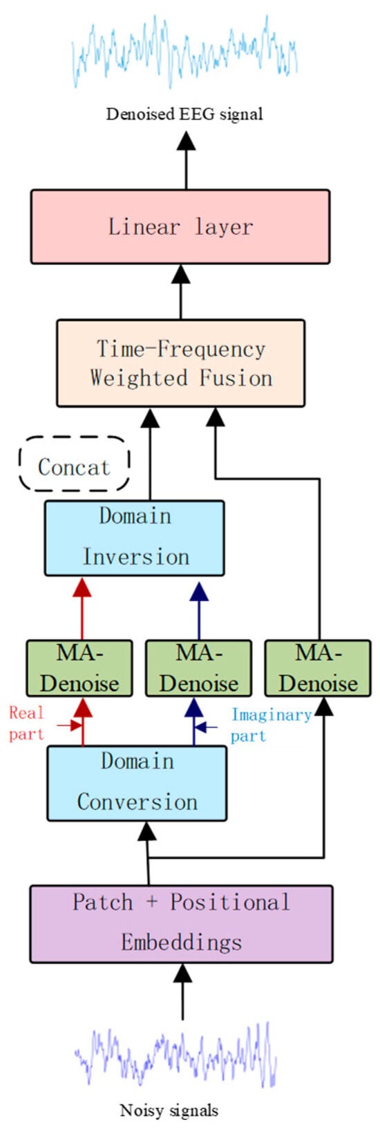
Figure 1. Model architecture diagram.

2.1. Signal Embedding

The signal embedding process in the module is carried out through patching and linear mapping operations to capture and enhance the temporal features from the input signal, thereby improving the processing capacity of subsequent network layers. First, the input signal s is divided into multiple smaller patches through a patching operation, resulting in a patched sequence s’, The sequence then passes through two linear layers, a GELU activation function, and a dropout layer. These operations map the input signal into a higher-dimensional space (mini_seq * hidden_dim), generating the embedded feature S, which typically has a larger dimension than the original input. This approach ensures preservation of the signal’s local information, and richer features are presented in the higher-dimensional space, which helps the subsequent network layers perform better feature extraction and signal recovery.

2.2. Denoising Module

The attention mechanism can effectively extract data features [34,35]. In this study, a multi-attention denoising module (MA-Denoising) is proposed, as illustrated in Figure 2. To simultaneously capture local and global features in EEG signals, we design the MA-denoise module. Specifically, the Simplified Linear Attention (SLA) employs the ReLU kernel function to efficiently model long-range dependencies for extracting global context. Meanwhile, the Channel Reduction Attention (CRA) compresses the channel dimensions of queries and keys into one dimension, maintaining spatial detail perception ability to enhance local features while significantly reducing computational overhead. By integrating SLA with CRA, the model is enabled to model global relationships and local details. On this basis, we adopt pre-normalisation and residual structures to improve the network’s stability.

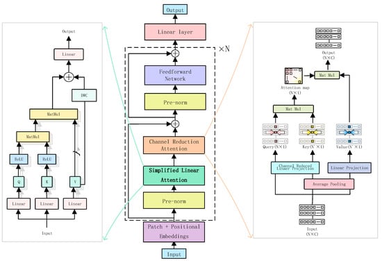
Figure 2. Denoising model architecture diagram.

2.2.1. Simplified Linear Attention

The attention mechanism is regarded as the key element in Transformer networks. The general form of self-attention is as follows. Given the input of N tokens $x\in R^{C\times C}$, self-attention in each head can be written as:

$$\begin{array}{cc}& Q=x{W}_Q,K=x{W}_K,V=x{W}_V,\\ & O_i={\displaystyle \sum _{j=1}^N}{\displaystyle \frac{Sim\left(Q_i,K_j\right)}{{\sum }_{j}Sim\left(Q_i,K_j\right)}}{V}_j,\end{array}$$

(1)

where $W_Q,W_K,{and W}_V\in R^{C\times C}$ are the projection matrices. $Sim\left(\cdot ,\cdot \right)$ represents the similarity function. The Transformer typically uses Softmax attention, where the similarity measurement is defined as:

$${Sim}_{\mathrm{softmax}}\left(Q_i,K_j\right)=\mathrm{e}\mathrm{x}\mathrm{p}\left({\displaystyle \frac{Q_i{K}_j^T}{\sqrt{C}}}\right)$$

(2)

In this case, the attention map is obtained by computing the similarity between all query-key pairs, resulting in a computational complexity of O(N2). Traditional Softmax-based attention calculations have high computational complexity. Since we need to process the signal separately in the frequency and temporal domains, it may result in resource constraints. The core idea of SLA is to replace the Softmax similarity computation with a dot product calculation using the ReLU activation function while introducing the Depth-Wise Convolution (DWC) module to further enhance the modeling of local features. This approach achieves lower computational complexity and higher feature representation ability. The core formula is as follows:

$$\begin{array}{l}{Sim}_{SLA}(Q_i,K_j)=\mathrm{R}\mathrm{e}\mathrm{L}\mathrm{U}\left(Q_i\right)\mathrm{R}\mathrm{e}\mathrm{L}\mathrm{U}(K_j{)}^T,\hfill \\ {\tilde{O}}_i={\displaystyle \sum _{j=1}^N}{\displaystyle \frac{{\mathit{Sim}}_{\mathit{SLA}}\left(Q_i,K_j\right)}{{\sum }_{j=1}^N{\mathit{Sim}}_{\mathit{SLA}}\left(Q_i,K_j\right)}}{V}_j,\hfill \\ O_{SLA}=\tilde{O}+DWC\left(V\right)\end{array}$$

(3)

where $DWC(·)$represents Depth-Wise Convolution. Simplified Linear Attention (SLA) is essentially a global feature modeling mechanism.

However, in EEG artifact removal, by employing a local window partitioning strategy and depth-wise separable convolution modules, the approach effectively enhances the extraction and representation of local features, addressing the dense spatial distribution of artifacts in EEG signals. This combination not only reduces computational complexity but also adapts to the spatiotemporal dynamic characteristics of EEG data.

2.2.2. Channel Reduction Attention

After the local feature extraction module, the CRA performs deep optimisation on the extracted features. First, the features are dimensionally reduced and reconstructed through query, key, and value mappings. Then, it utilises an attention mechanism to generate weighted feature representations. Furthermore, multi-head attention interactions are employed to enhance the model’s capacity to capture both local and global patterns.

Average pooling is applied to the key and value before the attention mechanism, and the channel dimensions of the query and key are reduced to one dimension to reduce computational cost. We found that channel compression of the $Q\in R^{Head\times H_i\times W_i\times 1}$ and $K\in R^{Head\times \left({\displaystyle \frac{H_i{W}_i}{r_i^2}}\right)\times 1}$ effectively captures global similarity. The CRA operation is as follows:

$$\begin{array}{cc}& CRA\left(F_i\right)=Concat\left({Head}_0,\dots ,{Head}_j\right)W_i^O,\hfill \\ & Q_i=F_i{W}_j^Q,K_i=AvgPool\left(F_i\right)W_j^K,\hfill \\ & V_i=AvgPool\left(F_i\right)W_j^V,{Head}_j=Att\left(Q_i,K_i,V_i\right),\hfill \\ & Att\left(Q_i,K_i,V_i\right)=Softmax\left(Q_i{K}_i^T\right)V_i,\hfill \end{array}$$

(4)

where $W_j^Q,W_j^K\in R^{C_i\times 1},W_j^V\in R^{C_i\times {\displaystyle \frac{C_i}{j}}}$, and $W^O\in R^{C_i\times {\displaystyle \frac{C_i}{j}}}$ are the projection parameters. Here, $j$ denotes the number of attention heads. $AvgPool$ represents the average pooling at each stage with scales $ri\in \mathrm{2,4},8$. The computational complexity of CRA is:

$$\begin{array}{l}{N}^{\prime }={\displaystyle \frac{N}{r_i}},\\ \Omega \left(SRA\right)=(N^{\prime }{)}^{2}C+(N^{\prime }{)}^{2}C,\\ \Omega \left(CRA\right)=(N^{\prime }{)}^2\cdot 1+(N^{\prime }{)}^{2}C,\end{array}$$

(5)

where $N$ epresents the number of signal blocks. The two sides of Equation (5) correspond to the computations for the query-key operation and the attention weight operation, respectively. By reducing the computational cost of the query-key operation by a factor of $C$, the CRA reduces the total computational cost of the attention operation by approximately half.

Given that the input $S$ has the shape [B, mini_seq, hidden_dim], where mini_s eq represents the number of channels and hidden_dim denotes the number of features. After processing through the attention mechanism, the final output is the weighted and aggregated representation of the EEG signal across all channels. CRA adaptively weights each channel by computing attention, enhancing important channels (i.e., the most relevant mini-blocks) and reducing the influence of irrelevant or redundant channels. By weighted aggregation, CRA further improves signal quality and helps eliminate EEG contaminants, such as EOG and EMG.

2.3. Frequency Domain Transformation Module

The waveform we usually observe is the signal’s representation in the time domain. EEG signals represent potential fluctuations that vary over time along the time axis. While this representation effectively captures the temporal dynamics of the signal, it does not inherently support direct separation of distinct frequency components. To address this limitation, the time-domain signal is converted into its frequency-domain representation using the Fast Fourier Transform (FFT). In the frequency domain, distinct signal components often exhibit unique frequency characteristics, thereby facilitating their differentiation and subsequent processing.

Following the domain transformation, the signal’s real and imaginary parts are independently input into a deep learning network for training. Through this operation, the model can learn specific patterns of artifact signals and target signals in the frequency domain. Notably, the deep learning network performs nonlinear modeling of the signal’s frequency-domain characteristics at this stage, overcoming the limitations of traditional frequency-domain filtering methods that rely on linear assumptions. This enhances the accuracy of artifact removal.

Therefore, we convert the input S into the frequency domain $F$ as follows:

$$\begin{array}{c}F\left(f\right)={\int }_{-\infty }^{\infty }S\left(v\right)e^{-j2\pi fv}dv\\ ={\int }_{-\infty }^{\infty }S\left(v\right)cos\left(2\pi fv\right)dv\\ +j{\int }_{-\infty }^{\infty }S\left(v\right)sin\left(2\pi fv\right)dv\end{array}$$

(6)

where $f$ is the frequency variable, $v$ is the integration variable, and $j$ is the imaginary unit, defined as the square root of −1. The term ${\int }_{-\infty }^{\infty }S\left(v\right)cos\left(2\pi fv\right)dv$ represents the real part of $S$, abbreviated as $Re\left(F\right),{\int }_{-\infty }^{\infty }S\left(v\right)sin\left(2\pi fv\right)dv$ represents the imaginary part of S, abbreviated as $Im\left(F\right)$, We can then rewrite $F$ in Equation (6) as $F=Re\left(F\right)+jIm\left(F\right)$. After learning in the frequency domain, we use the following inverse transformation formula to convert F back to the time domain:

$$\begin{array}{c}S\left(v\right)={\int }_{-\infty }^{\infty }F\left(f\right)e^{j2\pi fv}df \\ ={\int }_{-\infty }^{\infty }\left(Re\left(F\left(f\right)\right)+jIm\left(F\left(f\right)\right)\right)e^{j2\pi fv}df\end{array}$$

(7)

We input the frequency-domain signal $F\left(f\right)$ into the denoising model for training to remove specific artifact-related frequency components. Subsequently, the processed frequency-domain signal $F\left(f\right)$ is transformed back into the time domain using Equation (7), resulting in the artifact-free, denoised signal $S\left(v\right)$.

2.4. Fusion Module

To fuse EEG features from both the time and frequency domains, we employ a lightweight yet efficient feature fusion module. This module dynamically adjusts the weights of representations from distinct domains through an adaptive attention mechanism, exploiting the complementary strengths of temporal and spectral signals.

The inputs to the module are the time-domain features $F_{time}\in R^{B\times C\times L}$ and the frequency-domain features $F_{freq}\in R^{B\times C\times L}$, where $B$ represents the batch size, $C$ denotes the size of each block, and $L$ is the sequence length. The weighting coefficients for the time-domain and frequency-domain features are computed through two independent linear layers. The weights $\alpha$ and $\beta$ are obtained by applying the Sigmoid activation function to the outputs of the linear layers, as follows:

$$\alpha =\sigma \left(W_{time}{F}_{time}\right)$$

(8)

$$\beta =\sigma \left(W_{freq}{F}_{freq}\right)$$

(9)

Here, $W_{time},W_{freq}\in R^{C\times C}$ are learnable weight matrices, and $\sigma \left(\cdot \right)$ denotes the Sigmoid activation function.

The computed weights $\alpha$ and $\beta$ are used to modulate the contributions of the time-domain and frequency-domain features to the final fused representation. By applying a weighted sum to the temporal and spectral features, we obtain the fused feature $F\_fused$ as follows:

$$F_{fused}=\alpha \odot F_{time}+\beta \odot F_{freq}$$

(10)

where ⊙ denotes element-wise multiplication. This weighted fusion process enables the module to adaptively adjust the fusion ratio between temporal and spectral features according to the features of the input. In the context of artifact removal tasks in EEG, the module selectively enhances the most relevant features by adaptively fusing time and frequency domains, thereby enhancing the effectiveness of artifact removal.

3. Dataset and Evaluation Methods

3.1. Dataset Introduction

3.1.1. Benchmark EEG Datasets for Simulated Artifact Contamination

To evaluate the effectiveness of our method, we conducted training and testing using a publicly available dataset from the EEGDiR model. This dataset is based on the EEGDenoiseNet dataset, which is widely utilised in deep learning approaches for EEG signal denoising. This dataset was collected from 52 healthy subjects performing left/right hand motor imagery tasks, using a 64-channel recording system. The raw signals were processed with band-pass filtering, power-line notch filtering, and downsampling. Independent components were labeled via ICA and the ICLabel tool to obtain clean data. Corresponding electrooculographic (EOG) and electromyographic (EMG) noises were derived from independently collected dedicated datasets. Specifically, the datasets contain 4515 noise-free EEG signals, 3400 ocular artifacts, and 5598 muscular artifacts. Each sample has a duration of 2 s with a sampling rate of 256 Hz. From the 4515 clean EEG signals, 3400 samples were randomly selected. Clean EEG signals were linearly combined with EOG signals at specific signal-to-noise ratio (SNR) levels ranging from −7 dB to 2 dB, to generate EEG signals contaminated with EOG artifacts. The resulting dataset was split into training and testing sets in a ratio of 8:2 and named the EOG Dataset 1. Similarly, EMG artifacts were randomly superimposed onto clean EEG signals to produce muscle-contaminated EEG data, referred to as the EMG Dataset. In addition, a semi-simulated EEG dataset (SS2016) contaminated with EOG artifacts was employed. EEG data were collected from 54 subjects in the eyes-closed resting state, using a 19-channel EEG system arranged based on the international 10–20 system with a sampling frequency of 200 Hz. The signals were segmented into epochs, each consisting of 512 sampling points. The dataset contains both clean and artifact-contaminated EEG signals. After preprocessing and removal of poor-quality samples, a total of 6716 samples were retained. Similarly, noise-free EEG signals are combined with ocular artifacts to generate signals contaminated by ocular artifacts, and this dataset is denoted as EOG Dataset 2. The generated dataset is split into the training set and test set at an 8:2 ratio.

3.1.2. Physio-Realistic Multi-Channel Semi-Simulated EOG Dataset

In this study, a multi-channel semi-simulated EEG/EOG dataset is utilised [36], which includes 19-channel EEG and EOG recordings from 27 healthy subjects. Each subject provided two segments of experimental data: one segment of artifact-free EEG signals collected under eyes-closed conditions, and the other segment of natural eye movement signals acquired under eyes-open conditions. The EEG signals were sampled at 200 Hz and processed with a 0.5–40 Hz bandpass filter and a 50 Hz power-line filter. EOG signals were collected via supraorbital, infraorbital, and lateral orbital electrodes on both sides, yielding two bipolar channels: vertical EOG (VEOG) and horizontal EOG (HEOG). Unlike traditional simulation methods, this dataset adopts a contamination approach based on a realistic physiological model, where clean EEG signals recorded under eyes-closed conditions are linearly superimposed with natural eye movement EOG signals from the same subject. This generates semi-simulated EEG signals with realistic physiological characteristics while retaining clean references. Contamination coefficients were obtained through linear regression based on the amplitude characteristics of EOG signals from subjects under eyes-open conditions, aiming to verify the generalisation ability of the proposed model under more complex electrode layouts and conditions closer to real-world scenarios.

3.2. Evaluation Metrics

We assessed the model using time-domain relative root mean square error (RRMSEt), frequency-domain relative root mean square errors (RRMSEs), signal-to-noise ratio (SNR), and correlation coefficient (CC).

RRMSE quantifies the difference between the predicted EEG signals and the noise-free signals. We calculated RRMSE in both the time domain and the spectral domain. The calculation formulas are as follows:

$$RMS\left(x\right)=\sqrt{{\displaystyle \frac{1}{C\cdot T}}{\displaystyle \sum _{c=0}^{C-1}}{\displaystyle \sum _{t=0}^{T-1}}{x}_{c,t}^2}$$

(11)

$$RRMS{E}_t={\displaystyle \frac{RMS\left(x_g-x\right)}{RMS\left(x\right)}}$$

(12)

$$RRMS{E}_s={\displaystyle \frac{RMS\left(PSD\left(x_g\right)-PSD\left(x\right)\right)}{RMS\left(PSD\left(x\right)\right)}}$$

(13)

where PSD represents the power spectral density of the input signal.

CC measures the linear correlation between the clean and contaminated EEG. The CC is defined as:

$$CC={\displaystyle \frac{Cov\left(\tilde{x},x\right)}{\sqrt{Var\left(\tilde{x}\right)Var\left(x\right)}}}$$

(14)

where, Cov denotes covariance, Var represents variance.

SNR measures the proportion of the clean signal relative to the background noise. The calculation formula is as follows:

$$\mathrm{SNR} \left(\mathrm{dB}\right)=10{\mathit{log}}_{10}\left({\displaystyle \frac{\sum _{i=1}^N{x}_i^2}{\sum _{i=1}^N({\tilde{x}}_i-x_i{)}^2}}\right)$$

(15)

4. Experiments and Results

4.1. Implementation Details

We designed the model based on the PyTorch (version 1.9.1) framework, adopting a training scheme of 3000 epochs with a batch size of 1000. For EOG, the learning rate was set to 1 × 10⁻⁴, while for EMG, it was set to 5 × 10⁻⁴. Due to the distinct characteristics of EOG and EMG signals, we adopted different learning rates, with the comparison results shown in Supplementary Table S1. The AdamW optimiser was employed with betas parameters ranging from (0.5, 0.9).

4.2. Results

To assess how effectively different methods remove artifacts from the EOG and EMG datasets, we conducted a comparison with SCNN, FCNN, RNN, EEGDnet, and EEGDiR using four metrics: RRMSEt, RRMSEs, CC, and SNR.

4.2.1. Results of the Benchmark EEG Dataset for Simulated Artifact Contamination

Table 1 presents the average artifact removal performance of different methods under various SNR levels across different datasets. Our method achieves either the lowest or second-lowest values in the RRMSEt and RRMSEs metrics, indicating its superior accuracy in reconstructing the original signal. The proposed model demonstrates more efficient feature extraction and stronger nonlinear fitting capabilities, which contribute to reduced reconstruction errors.

Table 1. The results of the proposed method validated on different datasets.

Dataset	Evaluation	SCNN	FCNN	RNN	EEGDnet	EEGDiR	Ours
EOG Dataset 1	RRMSEt	0.3877	0.4394	0.4602	0.3595	0.3724	0.3026
	RRMSEs	0.4072	0.4590	0.4867	0.3646	0.4019	0.3241
	CC	0.9100	0.8862	0.8802	0.9254	0.9145	0.9415
	SNR	9.0444	7.9920	7.4511	9.5408	9.6397	11.6260
EMG Dataset	RRMSEt	0.7092	0.5976	0.6310	0.6094	0.5316	0.5191
	RRMSEs	0.7021	0.6331	0.6307	0.5416	0.5539	0.5334
	CC	0.7276	0.7916	0.7570	0.7750	0.8115	0.8203
	SNR	3.6991	5.0817	4.6239	4.8732	6.9433	7.0262
EOG Dataset 2	RRMSEt	0.4619	0.5632	0.4907	0.3640	0.2790	0.2754
	RRMSEs	0.5658	0.5930	0.5163	0.4295	0.3370	0.3465
	CC	0.8839	0.8394	0.8799	0.9300	0.9594	0.9611
	SNR	7.4065	5.2437	6.4943	9.4262	11.9243	12.0611

Note. Boldface indicates the best results.

In terms of the CC metric, our method achieves the highest values across all datasets, suggesting a closer match between the reconstructed signals and the ground truth. Additionally, our method yields the highest post-denoising SNR across all datasets, highlighting its exceptional capability in noise suppression. Compared to other approaches, the proposed method more effectively filters out artifact-related noise and enhances the accuracy of signal reconstruction.

Figure 3 illustrates the evaluation metric results obtained by six different methods across ten different SNR between −7 dB and 2 dB. Overall, our method demonstrates superior artifact removal performance compared to the other approaches. It can be observed that denoising performance improves as the SNR increases. From the RRMSE plots, we can see that the error for all methods decreases with increasing SNR, indicating lower reconstruction errors under high-SNR conditions. However, the rate of error reduction varies among methods. Our proposed method (yellow curve) maintains lower errors even under low SNR conditions, suggesting stronger robustness in noisy environments. The CC trends show that the CC values for all methods increase with higher SNR, meaning that the correlation between denoised and clean signals improves as the signal becomes cleaner. Notably, our method maintains relatively high correlation even at low SNR levels, demonstrating its advantage in low-SNR scenarios. The rightmost subplots illustrate the post-denoising SNR results of different methods. Notably, FCNN exhibits relatively low denoised SNR even under high input SNR conditions. In contrast, the denoised SNR of the other methods increases as the SNR of the EEG signals increases.

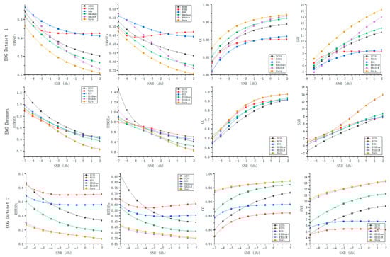
Figure 3. Denoising performance of different methods under various SNR levels across three datasets.

Figure 4 presents boxplots of all evaluation metrics for each test sample across three datasets using different methods. For the error metrics in the time and frequency domains, the sample distributions of all methods are relatively concentrated, while our method exhibits a lower mean and smaller variance, further demonstrating the stability of the proposed model in error control. Regarding the CC metric, comparative methods show significant fluctuations, whereas our model maintains a more compact distribution, reflecting more consistent signal recovery capability. In terms of the output SNR, especially in EOG Dataset 1, our method exhibits a higher signal-to-noise ratio, indicating that the proposed method can effectively remove artifacts.

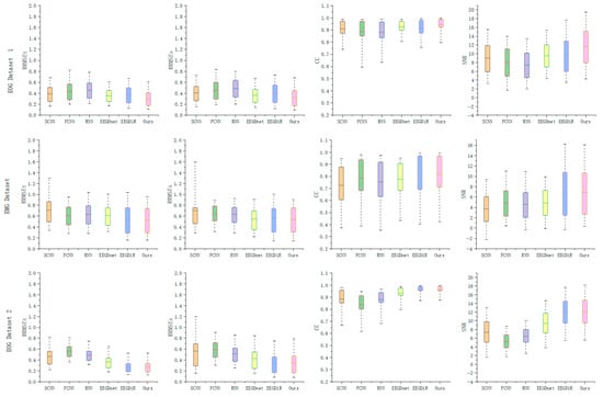
Figure 4. Boxplots of denoising performance using different methods across three datasets.

4.2.2. Results of the Physio-Realistic Multi-Channel Semi-Simulated EOG Dataset

The experiments on the multi-channel dataset adopted the same training strategy as the single-channel experiments. To adapt to the multi-electrode structure, this study treats each EEG channel as a minimal sequence of the model input, thereby explicitly preserving its spatial topological relationships in the network. Table 2 summarises the quantitative comparison results of different methods on the EOG dataset. Our method achieves the optimal performance across all evaluation metrics, demonstrating that the proposed method still maintains stable artifact removal performance under complex electrode layouts and conditions involving real ocular artifacts. The model can effectively reduce ocular artifacts in the multi-channel spatial dimension and recover the EEG morphology under the eyes-closed state.

Table 2. Validation of the proposed method on the multi-channel semi-simulated EEG dataset with realistic physiological characteristics.

Dataset	Evaluation	SCNN	FCNN	RNN	EEGDnet	EEGDiR	Ours
Semi-Simulated EOG Dataset	RRMSEt	0.9448	0.5438	0.6273	0.8785	0.3806	0.1870
	RRMSEs	0.9948	0.4926	0.5441	0.9801	0.7101	0.2566
	CC	0.7375	0.8403	0.7684	0.9759	0.9250	0.9761
	SNR	0.4953	5.7180	4.4817	1.1405	10.5187	17.3796

Note. Boldface indicates the best results.

4.3. Hyperparameter Analysis

To evaluate how network hyperparameters influence model performance, we conducted a systematic analysis of mini_seq, hidden_dim, and model depth on EOG Dataset 1 and the EMG Dataset, with the goal of determining the optimal configuration for the final model. Table 3 summarises the quantitative results obtained under different combinations of mini_seq and hidden_dim. As shown, larger hidden_dim values enhance the model’s representational capacity, whereas smaller dimensions lead to insufficient encoding of temporal and spectral information, indicating that higher feature dimensionality is essential for capturing richer time–frequency structures. In the EOG dataset, a mini_seq length of 16 consistently yielded superior performance under matched hidden_dim settings, suggesting that finer temporal segmentation more effectively describes the local dynamics of EOG signals. In contrast, EMG artefacts exhibit faster temporal fluctuations and broader spectral content, and thus benefit from a longer temporal window that captures contextual dependencies across local segments.

Table 3. Influence of mini_seq and hidden_dim on artefact-removal performance. The model uses 4 layers and 8 attention heads.

mini_seq	hidden_dim	EOG Dataset 1				EMG Dataset
		RRMSEt	RRMSEs	CC	SNR	RRMSEt	RRMSEs	CC	SNR
16	512	0.3026	0.3241	0.9415	11.6260	0.5368	0.5589	0.8110	6.6784
16	256	0.3165	0.3224	0.9405	11.5050	0.5584	0.5929	0.7976	6.2367
16	128	0.3230	0.3281	0.9398	11.4962	0.5893	0.5906	0.7650	5.6488
16	64	0.3394	0.3314	0.9379	11.3886	0.6256	0.5678	0.7328	5.1956
32	512	0.3056	0.3244	0.9406	11.6006	0.5191	0.5334	0.8203	7.0262
32	256	0.3090	0.3313	0.9390	11.5127	0.5397	0.5376	0.8023	6.6715
32	128	0.3113	0.3373	0.9355	11.5033	0.5789	0.5862	0.7766	5.8301
32	64	0.3196	0.3457	0.9348	11.4514	0.6205	0.5708	0.7444	5.1047

Note. Boldface indicates the best results.

Table 4 further reports the effect of model depth under fixed mini_seq and hidden_dim. Model performance improved steadily as the number of layers increased, demonstrating that deeper MA-denoise modules extract more informative representations and thereby strengthen artefact suppression.

Table 4. Influence of model depth on artefact-removal performance. The EOG dataset uses a mini_seq of 16, the EMG dataset uses a mini_seq of 32, and the model is configured with a hidden dimension of 512, 4 layers, and 8 attention heads.

Layers	EOG Dataset 1				EMG Dataset
	RRMSEt	RRMSEs	CC	SNR	RRMSEt	RRMSEs	CC	SNR
4	0.3026	0.3241	0.9415	11.6260	0.5191	0.5334	0.8203	7.0262
3	0.3085	0.3245	0.9382	10.6113	0.5252	0.5397	0.8137	6.9631
2	0.3090	0.3350	0.9399	10.4360	0.5242	0.5369	0.8154	7.0025
1	0.3245	0.3530	0.9345	10.9479	0.5228	0.5378	0.8160	7.0216

Note. Boldface indicates the best results.

Based on the above results, the optimal performance is achieved when mini_seq 16 is used for the EOG Dataset, mini_seq 32 for the EMG Dataset, and hidden_dim 512 with 4 layers MA-denoise modules are uniformly adopted. This configuration serves as the default setting for subsequent experiments. For more details, please refer to Supplementary Table S2.

4.4. Ablation Study s

To investigate the effectiveness of each module in our model, we conducted ablation experiments using the EMG dataset and EOG Dataset 2. We evaluated the model performance under seven different configurations, as shown in Table 5. The experiments compared the contributions of the SLA and CRA modules in both the time and frequency domains. The performance evaluation metrics included time-domain relative root mean square error (RRMSEt), frequency-domain relative root mean square error (RRMSEs), correlation coefficient, and output signal-to-noise ratio.

Table 5. Ablation study results on EOG Dataset 1 and the EMG Dataset.

No.	Frequency Domain	Time Domain	SLA	CRA	EOG Dataset 1				EMG Dataset
					RRMSEt	RRMSEs	CC	SNR	RRMSEt	RRMSEs	CC	SNR
1	-	√	√	-	0.3355	0.3676	0.9278	10.8471	0.5400	0.5639	0.8066	6.6387
2	-	√	-	√	0.3068	0.3255	0.9402	11.5250	0.5497	0.5757	0.8081	6.5310
3	-	√	√	√	0.3042	0.3195	0.9410	11.6099	0.5461	0.5710	0.8098	6.4312
4	√	-	√	-	0.3413	0.3764	0.9249	10.6926	0.5335	0.5565	0.8143	6.7027
5	√	-	-	√	0.3095	0.3292	0.9379	11.5211	0.5407	0.5601	0.8123	6.5057
6	√	-	√	√	0.3083	0.3293	0.9383	11.5837	0.5413	0.5579	0.8121	6.4919
7	√	√	√	√	0.3026	0.3241	0.9415	11.6260	0.5191	0.5334	0.8203	7.0262

Note. Boldface indicates the best results. “√” indicates that the corresponding module is applied, while “-“ indicates that it is not applied.

In the configurations using only time-domain information (No. 1–3), the results show that for EOG Dataset 1, the performance degradation when only removing SLA (No. 2) is greater than that when removing CRA (No. 1), while the combination of the two attention modules (No. 3) achieves relatively optimal time-domain performance. In contrast, in EMG data, removing CRA (No. 1) has a more significant impact on performance than removing SLA (No. 2). This difference indicates that different artifact types in the time domain have varying degrees of dependence on attention mechanisms, with low-frequency-dominated ocular artifacts are more reliant on the channel compression capability of CRA, whereas in EMG scenarios with a wider spectral distribution, SLA is more conducive to capturing fast-varying components. In the configurations using only frequency-domain features (No. 4–6), the joint configuration of SLA and CRA (No. 6) performs best on both datasets. For configurations retaining only one attention module (No. 4, No. 5), the model’s artifact suppression capability decreases. When both are present, however, the amplitude and phase features in the frequency domain are more fully utilised. This result demonstrates that frequency-domain modeling has a more significant dependence on attention mechanisms.

When both time-domain and frequency-domain information are used with both types of attention modules enabled (No. 7), the model achieves the highest performance across all metrics. Compared with the optimal time-domain configuration (No. 3) and the optimal frequency-domain configuration (No. 6), the complete model further improves RRMSE, CC, and output SNR. This result indicates that the time domain and frequency domain provide complementary information. The joint modeling of both domains combined with multi-attention mechanisms can form a more stable and generalisable artifact suppression strategy.

5. Discussion

5.1. Visualisation of Artifact Removal Results

Figure 5 and Figure 6, respectively present the comparison results before and after artifact removal on EOG Dataset 1 and the EMG dataset. The figures display the best (highest correlation, left column) and worst (lowest correlation, right column) denoising waveforms achieved by different deep learning methods. It can be observed that all types of deep learning approaches are capable of effectively removing artifacts and reconstructing the target EEG signals. The samples in the left column represent EEG signals with higher SNR, while those in the right column have lower SNR. As shown in the figures, denoising results are clearly better in the high-SNR cases, indicating that SNR has a strong impact on denoising performance. The performance of all methods improves with increasing SNR. Under low SNR conditions, our method still maintains a relatively accurate trend and amplitude, effectively suppressing low-frequency drift characteristics and well preserving the intrinsic structure of EEG signals. Figure 7 and Figure 8 show the artifact removal results of the same data segment from EOG Dataset 1 and the EMG Dataset using different methods. It can be observed that our method demonstrates a relatively balanced performance in terms of signal smoothness and structural preservation.

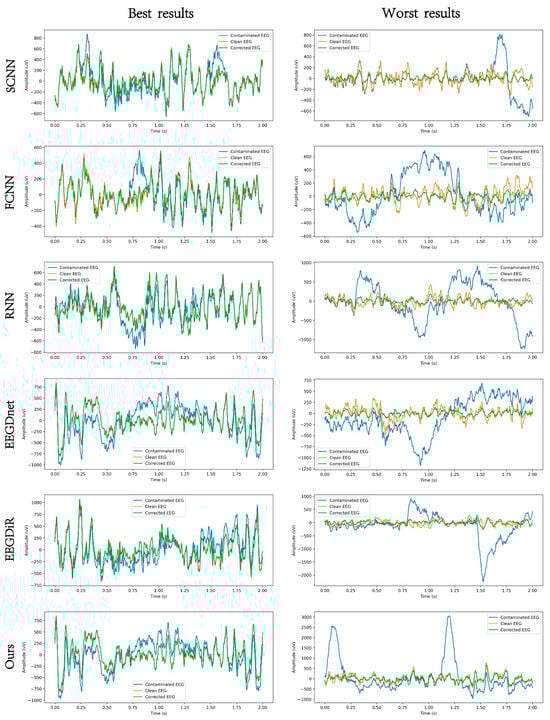
Figure 5. An example EEG segment demonstrating the results of EOG artifact removal under different models, where the orange, blue, and green lines represent the clean EEG, the contaminated EEG, and the corrected EEG, respectively.

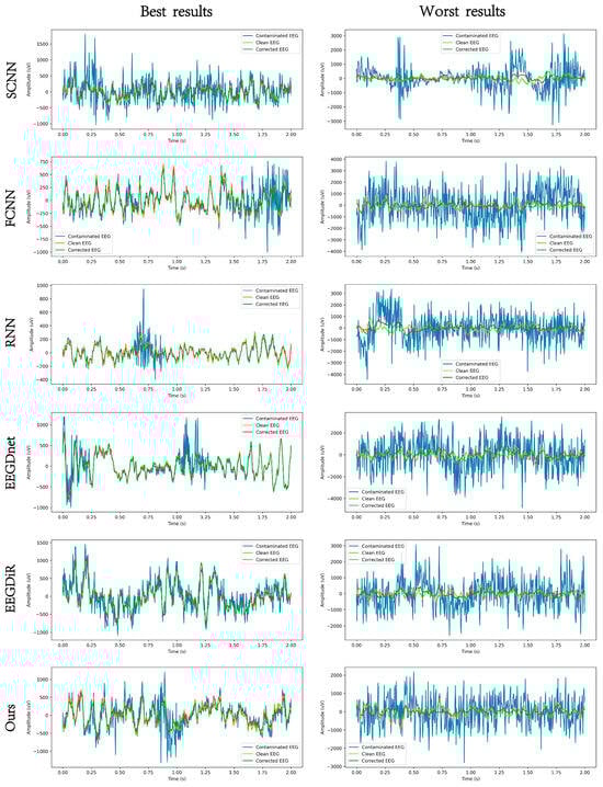
Figure 6. An example EEG segment demonstrating the results of EMG artifact removal under different models, where the orange, blue, and green lines represent the clean EEG, the contaminated EEG, and the corrected EEG, respectively.

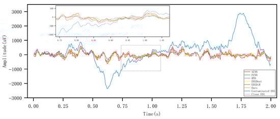
Figure 7. Visualisation of artifact removal results on the same EOG data segment using different methods.

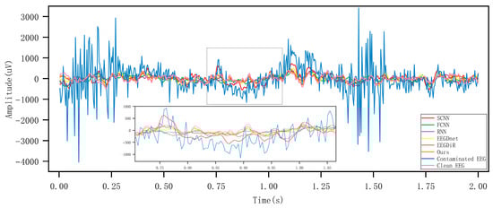
Figure 8. Visualisation of artifact removal results on the same EMG data segment using different methods.

5.2. Comparison and Advantage Analysis of Feature Extraction Methods

SCNN extracts local time-domain features through 1D convolutional layers but fails to effectively capture frequency-domain information. RNN by learning long-term and short-term dependencies, processes sequential data but neglects frequency-domain features and is susceptible to gradient vanishing issues. FCNN extracts temporal features through fully connected layers but lacks effective modeling of temporal dependencies. EEGDNet uses the self-attention mechanism of Transformers to extract time-domain and non-local features but does not fully consider frequency-domain information. EEGDiR extracts local features using Retentive Networks and multi-scale retention but remains confined to the time domain.

In contrast, we apply the Fourier transform to convert time-domain signals into the frequency domain, obtaining a complex representation composed of real and imaginary parts. The real part corresponds to the cosine components of each frequency, while the imaginary part corresponds to the sine components, together capturing the amplitude and phase information across different frequency bands. In frequency-domain modeling, we directly use the real and imaginary parts of the complex spectrum as the network’s inputs and outputs. Since the real and imaginary parts are continuous real-valued signals, this makes the network’s regression training more stable. Finally, the predicted real and imaginary parts are recombined into a complete complex spectrum and transformed back into the time domain via the inverse Fourier transform, ensuring that the reconstructed signal retains both amplitude and phase information.

We effectively extract frequency-domain features through Fourier transform and, in combination with the SLA and CRA modules, delve into both local and global features in the time and frequency domains. This overcomes the limitations of other models in processing both time and frequency domains, offering more comprehensive feature extraction and superior denoising performance.

5.3. Computational Efficiency Comparison

We compared the number of parameters and the computation time required to process a single test sample across different models. Table 6 provides the network parameters and inference times for the proposed denoiser and five comparison methods on the EOG artifact removal task (2-s, 256 Hz EEG segments). For the inference time calculation, a single run test samples, and the average value was obtained.

Table 6. Number of parameters and testing time for different models.

Methods	Parameter (×106)	Inference Time (ms)
SCNN	16.82	2.45
FCNN	1.05	0.15
RNN	2.89	0.61
EEGDnet	0.18	1.33
EEGDiR	80.79	29.09
Ours	96.66	28.52

The proposed method requires 96.66 million parameters for EOG artifact removal. Our model’s higher complexity stems from independently analyzing EEG signals in the time and frequency domains, which enhances its ability to learn complex patterns.

Our model’s computation time is 28.52 ms. The processing times, though higher than those of competing models, are comfortably within the 2000 ms input window, maintaining the model’s capability for real-time EEG analysis. Importantly, the proposed method demonstrates better average denoising performance than the baseline models, illustrating the inherent trade-off between processing efficiency and accuracy.

6. Conclusions

This paper presents MD-Denoiser, a deep learning model designed with a joint time–frequency optimisation strategy for EEG artifact removal. The model strengthens the temporal representation of EEG signals via a position embedding module. By applying the Fast Fourier Transform (FFT), EEG signals are transformed from the time domain into the complex frequency domain, where the real and imaginary components are denoised separately. Furthermore, the proposed multi-attention denoising (MA-Denise) module simultaneously captures local and global features, effectively eliminating ocular and muscular artifacts. This method enhances the robustness of EEG denoising and contributes to the stability of EEG-related systems.

References

- Cohen, M.X. Where Does EEG Come From and What Does It Mean? Trends Neurosci. 2017, 40, 208–218. [Google Scholar] [CrossRef]
- Coyle, S.M.; Ward, T.E.; Markham, C.M. Brain–Computer Interface Using a Simplified Functional near-Infrared Spectroscopy System. J. Neural Eng. 2007, 4, 219. [Google Scholar] [CrossRef]
- Ponten, S.C.; Daffertshofer, A.; Hillebrand, A.; Stam, C.J. The Relationship between Structural and Functional Connectivity: Graph Theoretical Analysis of an EEG Neural Mass Model. Neuroimage 2010, 52, 985–994. [Google Scholar] [CrossRef]
- Naeem, M.; Brunner, C.; Leeb, R.; Graimann, B.; Pfurtscheller, G. Seperability of Four-Class Motor Imagery Data Using Independent Components Analysis. J. Neural Eng. 2006, 3, 208. [Google Scholar] [CrossRef]
- Cui, H.; Liu, A.; Zhang, X.; Chen, X.; Liu, J.; Chen, X. EEG-Based Subject-Independent Emotion Recognition Using Gated Recurrent Unit and Minimum Class Confusion. IEEE Trans. Affect. Comput. 2022, 14, 2740–2750. [Google Scholar] [CrossRef]
- Tzallas, A.T.; Tsipouras, M.G.; Fotiadis, D.I. Epileptic Seizure Detection in EEGs Using Time–Frequency Analysis. IEEE Trans. Inf. Technol. Biomed. 2009, 13, 703–710. [Google Scholar] [CrossRef]
- Arpaia, P.; Moccaldi, N.; Prevete, R.; Sannino, I.; Tedesco, A. A Wearable EEG Instrument for Real-Time Frontal Asymmetry Monitoring in Worker Stress Analysis. IEEE Trans. Instrum. Meas. 2020, 69, 8335–8343. [Google Scholar] [CrossRef]
- Chen, X.; Liu, A.; Chiang, J.; Wang, Z.J.; McKeown, M.J.; Ward, R.K. Removing Muscle Artifacts from EEG Data: Multichannel or Single-Channel Techniques? IEEE Sens. J. 2015, 16, 1986–1997. [Google Scholar] [CrossRef]
- Touil, M.; Bahatti, L.; El Magri, A. Sleep’s Depth Detection Using Electroencephalogram Signal Processing and Neural Network Classification. J. Med. Artif. Intell. 2022, 5, 9. [Google Scholar] [CrossRef]
- Balaji, A.; Tripathi, U.; Chamola, V.; Benslimane, A.; Guizani, M. Toward Safer Vehicular Transit: Implementing Deep Learning on Single Channel EEG Systems for Microsleep Detection. IEEE Trans. Intell. Transp. Syst. 2021, 24, 1052–1061. [Google Scholar] [CrossRef]
- Chien, Y.-R.; Wu, C.-H.; Tsao, H.-W. Automatic Sleep-Arousal Detection with Single-Lead EEG Using Stacking Ensemble Learning. Sensors 2021, 21, 6049. [Google Scholar] [CrossRef] [PubMed]
- Li, Y.; Liu, A.; Yin, J.; Li, C.; Chen, X. A Segmentation-Denoising Network for Artifact Removal from Single-Channel EEG. IEEE Sens. J. 2023, 23, 15115–15127. [Google Scholar] [CrossRef]
- Gratton, G.; Coles, M.G.; Donchin, E. A New Method for Off-Line Removal of Ocular Artifact. Electroencephalogr. Clin. Neurophysiol. 1983, 55, 468–484. [Google Scholar] [CrossRef]
- Yadav, S.; Saha, S.K.; Kar, R. Evolutionary Algorithm-Based Optimal Wiener-Adaptive Filter Design: An Application on Eeg Noise Mitigation. IEEE Trans. Instrum. Meas. 2023, 72, 4011912. [Google Scholar] [CrossRef]
- Krishnaveni, V.; Jayaraman, S.; Anitha, L.; Ramadoss, K. Removal of Ocular Artifacts from EEG Using Adaptive Thresholding of Wavelet Coefficients. J. Neural Eng. 2006, 3, 338. [Google Scholar] [CrossRef]
- Chen, X.; Peng, H.; Yu, F.; Wang, K. Independent Vector Analysis Applied to Remove Muscle Artifacts in EEG Data. IEEE Trans. Instrum. Meas. 2017, 66, 1770–1779. [Google Scholar] [CrossRef]
- Chen, X.; Wang, Z.J.; McKeown, M. Joint Blind Source Separation for Neurophysiological Data Analysis: Multiset and Multimodal Methods. IEEE Signal Process. Mag. 2016, 33, 86–107. [Google Scholar] [CrossRef]
- Wang, G.; Teng, C.; Li, K.; Zhang, Z.; Yan, X. The Removal of EOG Artifacts from EEG Signals Using Independent Component Analysis and Multivariate Empirical Mode Decomposition. IEEE J. Biomed. Health Inform. 2015, 20, 1301–1308. [Google Scholar] [CrossRef]
- Chen, X.; Liu, Q.; Tao, W.; Li, L.; Lee, S.; Liu, A.; Chen, Q.; Cheng, J.; McKeown, M.J.; Wang, Z.J. ReMAE: User-Friendly Toolbox for Removing Muscle Artifacts from EEG. IEEE Trans. Instrum. Meas. 2019, 69, 2105–2119. [Google Scholar] [CrossRef]
- Kamath, V.; Lai, Y.-C.; Zhu, L.; Urval, S. Empirical Mode Decomposition and Blind Source Separation Methods for Antijamming with GPS Signals. In Proceedings of the IEEE/ION PLANS 2006, Coronado, CA, USA, 25–27 April 2006; pp. 335–341. [Google Scholar]
- Tian, C.; Fei, L.; Zheng, W.; Xu, Y.; Zuo, W.; Lin, C.-W. Deep Learning on Image Denoising: An Overview. Neural Netw. 2020, 131, 251–275. [Google Scholar] [CrossRef] [PubMed]
- Zhang, K.; Zuo, W.; Zhang, L. FFDNet: Toward a Fast and Flexible Solution for CNN-Based Image Denoising. IEEE Trans. Image Process. 2018, 27, 4608–4622. [Google Scholar] [CrossRef] [PubMed]
- Young, T.; Hazarika, D.; Poria, S.; Cambria, E. Recent Trends in Deep Learning Based Natural Language Processing. IEEE Comput. Intell. Mag. 2018, 13, 55–75. [Google Scholar] [CrossRef]
- Otter, D.W.; Medina, J.R.; Kalita, J.K. A Survey of the Usages of Deep Learning for Natural Language Processing. IEEE Trans. Neural Netw. Learn. Syst. 2020, 32, 604–624. [Google Scholar] [CrossRef]
- Zhang, H.; Zhao, M.; Wei, C.; Mantini, D.; Li, Z.; Liu, Q. EEGdenoiseNet: A Benchmark Dataset for Deep Learning Solutions of EEG Denoising. J. Neural Eng. 2021, 18, 056057. [Google Scholar] [CrossRef]
- Sun, W.; Su, Y.; Wu, X.; Wu, X. A Novel End-to-End 1D-ResCNN Model to Remove Artifact from EEG Signals. Neurocomputing 2020, 404, 108–121. [Google Scholar] [CrossRef]
- Sawangjai, P.; Trakulruangroj, M.; Boonnag, C.; Piriyajitakonkij, M.; Tripathy, R.K.; Sudhawiyangkul, T.; Wilaiprasitporn, T. EEGANet: Removal of Ocular Artifacts from the EEG Signal Using Generative Adversarial Networks. IEEE J. Biomed. Health Inform. 2021, 26, 4913–4924. [Google Scholar] [CrossRef]
- Zhang, Z.; Yu, X.; Rong, X.; Iwata, M. A Novel Multimodule Neural Network for Eeg Denoising. IEEE Access 2022, 10, 49528–49541. [Google Scholar] [CrossRef]
- Pu, X.; Yi, P.; Chen, K.; Ma, Z.; Zhao, D.; Ren, Y. EEGDnet: Fusing Non-Local and Local Self-Similarity for EEG Signal Denoising with Transformer. Comput. Biol. Med. 2022, 151, 106248. [Google Scholar] [CrossRef]
- Pei, Y.; Xu, J.; Chen, Q.; Wang, C.; Yu, F.; Zhang, L.; Luo, W. DTP-Net: Learning to Reconstruct EEG Signals in Time-Frequency Domain by Multi-Scale Feature Reuse. IEEE J. Biomed. Health Inform. 2024, 28, 2662–2673. [Google Scholar] [CrossRef]
- Wang, B.; Deng, F.; Jiang, P. EEGDiR: Electroencephalogram Denoising Network for Temporal Information Storage and Global Modeling through Retentive Network. Comput. Biol. Med. 2024, 177, 108626. [Google Scholar] [CrossRef]
- Xing, L.; Casson, A.J. Deep Autoencoder for Real-Time Single-Channel EEG Cleaning and Its Smartphone Implementation Using Tensorflow Lite with Hardware/Software Acceleration. IEEE Trans. Biomed. Eng. 2024, 71, 3111–3122. [Google Scholar] [CrossRef] [PubMed]
- Yi, K.; Zhang, Q.; Fan, W.; Wang, S.; Wang, P.; He, H.; An, N.; Lian, D.; Cao, L.; Niu, Z. Frequency-Domain MLPs Are More Effective Learners in Time Series Forecasting. Adv. Neural Inf. Process. Syst. 2023, 36, 76656–76679. [Google Scholar]
- Guo, J.; Chen, X.; Tang, Y.; Wang, Y. Slab: Efficient Transformers with Simplified Linear Attention and Progressive Re-Parameterized Batch Normalization. arXiv 2024, arXiv:2405.11582. [Google Scholar] [CrossRef]
- Kang, B.; Moon, S.; Cho, Y.; Yu, H.; Kang, S.-J. Metaseg: Metaformer-Based Global Contexts-Aware Network for Efficient Semantic Segmentation. In Proceedings of the IEEE/CVF Winter Conference on Applications of Computer Vision, Waikoloa, HI, USA, 3–8 January 2024; pp. 434–443. [Google Scholar]
- Klados, M.A.; Bamidis, P.D. A Semi-Simulated EEG/EOG Dataset for the Comparison of EOG Artifact Rejection Techniques. Data Brief 2016, 8, 1004–1006. [Google Scholar] [CrossRef] [PubMed]
Disclaimer/Publisher’s Note: The statements, opinions and data contained in all publications are solely those of the individual author(s) and contributor(s) and not of MDPI and/or the editor(s). MDPI and/or the editor(s) disclaim responsibility for any injury to people or property resulting from any ideas, methods, instructions or products referred to in the content. |
© 2025 by the authors. Licensee MDPI, Basel, Switzerland. This article is an open access article distributed under the terms and conditions of the Creative Commons Attribution (CC BY) license.