Infimum and Supremum of Thresholds for Reversible Data Hiding

Abstract

Reversible data hiding typically relies on two main techniques: prediction-error expansion and histogram shifting. These techniques complement each other to facilitate effective data embedding by defining non-positive and non-negative thresholds, thereby reducing distortion. The goal is to minimize overflow and underflow pixels by constraining thresholds appropriately. Managing these pixels remains challenging as they must be mapped within the payload. While double modification testing can eliminate the location map for some images, it is highly complex and struggles with images near intensity limits. In this paper, we show that the non-positive and non-negative thresholds for each predicted value are bounded by their infimum and supremum. By restricting the thresholds to these bounds, we maximize the number of embeddable pixels while minimizing the location map size. Moreover, our approach enables the rapid determination of the first operating thresholds and the development of encoding and decoding formulas for RDH without modification. Performance comparisons with established algorithms demonstrate the advantages of our proposed method.

1. Introduction

A significant challenge in data hiding is the distortion caused to the original media during the embedding process, which can make recovery impossible. This is particularly critical in applications like remote sensing, law enforcement, and medical imaging, where any distortion is unacceptable. Researchers have struggled to develop methods that eliminate distortion entirely. To tackle this issue, the reversible data hiding (RDH) technique was introduced, allowing for the complete recovery of both the host media and the embedded data. Over the past decade, numerous RDH methods have been proposed and refined to enhance their efficiency. These advancements have focused on increasing embedding capacity, reducing image degradation, and simplifying algorithm complexity. Among the most widely studied and continually improved techniques are lossless compression-based methods [1,2,3,4], difference expansion (DE) methods [5,6,7,8,9], histogram shifting (HS) methods [10], integer transform-based methods [11,12], and prediction-error expansion (PEE) methods [13,14,15,16,17,18,19,20,21,22,23,24].

DE, introduced by Tian [5], employs the Haar wavelet transform to process image data by decomposing it into low-pass and high-pass components. Bit shifting is applied to the pixel-pair differences in the high-pass image, creating vacant space in the least significant bit (LSB) to allow for additional data embedding. Despite its capability, this technique is hindered by high distortion and limited embedding capacity. Ni et al. [10] proposed the HS technique, where pixel values are shifted between the peak and zero-frequency bins of the histogram to embed data into mode-value pixels. However, the limited number of mode-value pixels constrains the payload capacity. PEE, introduced by Thodi et al. [13,14,15], expands prediction errors calculated from a predictor. This technique can be further enhanced by utilizing high-performance predictors.

A highly effective approach to data embedding, commonly utilized in recent studies, involves combining PEE with HS [14,15]. A notable advancement in this method is the work by Sachnev et al., which integrates multiple techniques, including a double-layer embedding scheme, rhombus predictor, double modification testing, and a sorting technique [7]. This combination achieved the highest performance reported to date. Building on this, Hwang et al. [19] further refined Sachnev et al.’s approach. Additionally, Li et al. [21] introduced two enhancements: the first involves embedding two bits in smooth regions and one bit in rough regions, offering superior performance for high payloads. The second is a pixel selection technique, which operates similarly to the sorting method. Coltuc [20] proposed a modified data embedding method to reduce the distortion by splitting the whole modified prediction-error into the embedded media and its prediction context. Coatrieux et al. [25] proposed to utilize the pixel histogram shifting and dynamic prediction-error in the low-high and intermediate predicted value locations, respectively. Li et al. [23] proposed a general framework of RDH and also presented two novel methods. The linear predictor with non-uniform weight achieved an excellent performance. Panyindee et al. [26] proposed a predictive model and an adaptive sorting method for each image and embedding size. Their work applied GA to determine the optimal parameters to achieve the lowest possible distortion.

In recent years, numerous RDH schemes [27,28,29,30,31] have been developed for colored images, broadening their range of applications. Among these, RDH in the encryption domain [28,29] has attracted significant attention. Qin et al. [28] introduced a separable RDH method for encrypted images, where a prediction strategy was employed at the receiver end to enable perfect image recovery. More recently, Li et al. [30,31] presented an innovative image steganography method that utilizes a decolorization network and a robust embedding algorithm, allowing for the embedding and extraction of secret data during the process of color translation. Several efficient RDH algorithms have been reported, including those for JPEG images [32,33,34,35,36,37,38,39], 3D mesh models [40,41,42], contrast enhancement [43,44], visible and invertible watermarking [45], video [46,47], and the human vision system (HVS) [48,49].

Although improvements to the RDH process are continuously being made in various aspects, the issue of overflow/underflow pixels (U_i,j < 0 and U_i,j > 255 in an 8-bit grayscale image) remains a significant challenge because these pixels need to be mapped and included as part of the payload for embedding. The double modification testing technique [17] has been reported to result in no location map for some images. However, this technique is highly complex and tends to encounter issues when applied to images with intensity values close to the maximum and minimum levels. Modifying every pixel twice, especially if the image has intensity values close to the maximum and minimum values, often causes overflow and underflow problems and requires the map to be stored. In this paper, we present a novel RDH scheme that performs effectively on two types of locations: those with similar intensities, such as in Man, Tiffany, etc., and those with differing intensities, as seen in Lena, Barbara, etc., which are close to the minimum (0) or maximum (255) values. All images mentioned above were downloaded from [50] except Barbara which was downloaded from [51]. The aim is to minimize overflow/underflow pixels by restricting thresholds within appropriate ranges. We have proposed a new embedding method that does not require single modification testing (SMT) or double modification testing (DMT), improving embedding efficiency even when pixel intensity values approach the maximum and minimum limits. Additionally, this method allows us to design a procedure for quickly determining the first operating thresholds and to develop encoding and decoding formulas for RDH based on PEE and HS.

This paper is organized as follows. Section 2 reviews related work. The overflow and underflow reduction are introduced in Section 3. The advantage of the infimum and supremum is presented in Section 4. Section 5 briefly describes the encoding and decoding. Section 6 provides experiments. Finally, Section 7 concludes the paper.

2. Related Work

The size of the location map is a primary concern in [5,7,13,14,15]. It is typically large and requires compression. However, even after compression, it still occupies a portion of the payload space. Therefore, the efficiency of the method depends on the size of the compressed location map. The overflow and underflow problem in the histogram shifting method is unavoidable, and pixels in the E and S sets that cause these errors should be excluded. The condition 0 ≤ u_i,j + D_i,j ≤ 255 is used to identify such problematic pixels, where D_i,j represents the modified error after data hiding through histogram shifting, either by shifting or expanding. This process is known as single modification testing (SMT), but a compression tool is still required for this method. In two-pass testing, the location map is significantly smaller or may not be needed. This approach, introduced by Sachnev et al. [17], checks whether a modified pixel’s value will lead to overflow or underflow by applying double expanding or shifting. Known as double modification testing (DMT), this method does not require compression for images where intensity values do not approach the maximum and minimum limits. However, for images with many pixels near these extreme values, DMT encounters significant overflow and underflow issues due to the second modification. A more detailed explanation of SMT and DMT, along with examples, will be provided in the next section. The comparison, as shown in Table 1, highlights the advantages of the proposed method over SMT and DMT.

Table 1. Comparison of the proposed method vs. SMT and DMT.

Criteria	Proposed Method	SMT [16,21,23]	DMT [17,19,26]
Location Map Size	Smaller or may not be required	Requires compression	Very small or not needed
Overflow/Underflow Handling	Effectively minimizes issues	Excludes problematic pixels	Encounters issues with extreme values
Embedding Efficiency	Higher due to reduced overhead	Limited by excluded pixels	Affected by second modification
Computational Complexity	Moderate	Low	High
Need for Compression Tool	Not required	Required	Not required for non-extreme images
Performance on Images with Extreme Intensity Values	More stable	Avoids modification of critical pixels	Faces significant issues

3. Overflow and Underflow Reduction

3.1. Common Techniques of RDH

This section serves as a review of basic techniques related to our proposal. The common techniques of RDH are PEE and HS [13,14,15]. This method involves breaking down an image pixel value u_i,j into a predicted value u′_i,j and a prediction error d_i,j, expressed as u_i,j = u′_i,j + d_i,j, where (i,j) indicates the pixel’s position. The predicted value is generally calculated based on the neighboring pixels. After obtaining the prediction error, it is expanded to create space for embedding the message. To minimize distortion caused by the expansion process, histogram shifting (HS) is applied to the pixels that do not contain embedded data. The following formula for RDH is based on PEE and HS:

$$U_{i,j}=\left\{\begin{array}{cc}{u}_{i,j}^{\prime }+d_{i,j}+t_p+1\hfill & if\hspace{1em}{d}_{i,j}>t_p\hfill \\ u_{i,j}^{\prime }+2d_{i,j}+b\hfill & if\hspace{1em}{d}_{i,j}\in \left[t_n,t_p\right]\hfill \\ u_{i,j}^{\prime }+d_{i,j}+t_n\hfill & if\hspace{1em}{d}_{i,j}<t_n.\hfill \end{array}\right.$$

(1)

The thresholds t_n and t_p represent the non-positive and non-negative values, respectively, while b denotes the data bit to be embedded. U_i,j refers to the modified pixel value. However, this formula cannot be applied universally to all pixels in the image due to potential underflow and overflow conditions, where U_i,j < 0 and U_i,j > 255 in an 8-bit grayscale image. To address this issue, certain pixels must remain unchanged and are recorded in the location map (a binary map that records the positions of modified pixels and identifies underflow or overflow issues) to ensure that the embedding process remains reversible.

Our approach focuses on minimizing the number of overflow and underflow pixels by constraining t′_n and t′_p within appropriate ranges. Here, t′_n and t′_p represent the non-positive and non-negative thresholds, respectively, for each predicted value u’, where u $\mathbf{\in }${ℤ: 0 ≤ u′ ≤ 255}. The smallest value within the range of t′_n is referred to as the infimum, while the largest value within the range of t′_p is known as the supremum.

By plugging b = 0 for d_i,j < 0 and b = 1 for d_i,j ≥ 0 into (1) (extreme of embedding), pixels that satisfy this equation without causing overflow or underflow issues are classified as expandable or shiftable pixels. Conversely, pixels that do not satisfy this condition are considered problematic pixels. This approach is known as the single modification testing (SMT) technique [16,21,23]. Similarly, if a pixel satisfies Equation (1) twice under extreme bit embedding without leading to overflow or underflow, it does not require marking in the location map. Otherwise, it is deemed a problematic pixel and must be marked in the location map. This process is referred to as the two-pass testing technique [17,19], also called the double modification testing (DMT) [26]. t′_n and t′_p are used to classify the sets of pixels with SMT or DMT. The cardinal number of each set is changed due to change in either t′_n or t′_p. The sets of image pixels are composed mainly of one carrying set (The pixels in this set can embed data), one non-carrying set (the pixels in this set cannot embed data) without the location map and one non-carrying set with the location map (overflow/underflow set or problematic set).

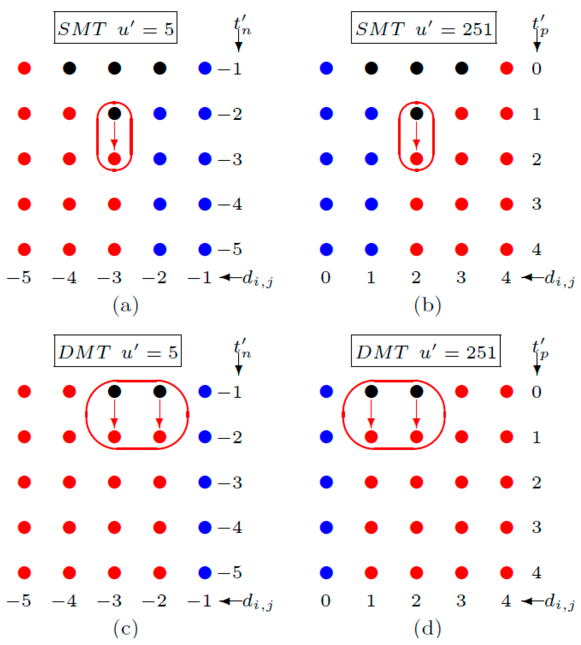
We provide the basic idea of our strategy before we prove the infimum and supreme for SMT and DMT. As we see in Figure 1a, it is obvious to us that the infimum for the SMT of u′ = 5 is −2 because the pixels, d_i,j = −3, transform into the member of a non-carrying set with the location map, when t′_n is decreased from −2 to −3. For DMT, u′ = 251, we can avoid increasing the member of a non-carrying set with location map by stopping t′_p at 0. Obviously, we have the largest number of a carrying set with the smallest possible size of a non-carrying set with the location map as long as t′_n and t′_p are stopped at its infimum and supremum. We can find the infimum and supremum for other predicted values, no doubt, by using the flowchart of SMT and DMT (Figure 2) to create the chart like the one shown in Figure 1.

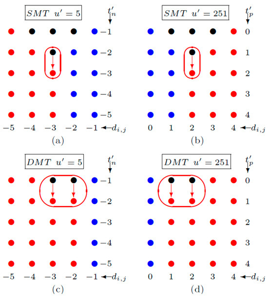
Figure 1. Example on the supremum and infimum strategy. To reduce the cardinality of a non-carrying set with the location map, the infimum of u′ = 5 is −2 for SMT (a) and −1 for DMT (c) and the supremum of u′ = 251 is 1 for SMT (b) and 0 for DMT (d). The red dots are the members of the non-carrying set with the location map. The black dots are the members of the non-carrying set without the location map. The blue dots are the members of the carrying set.

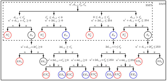
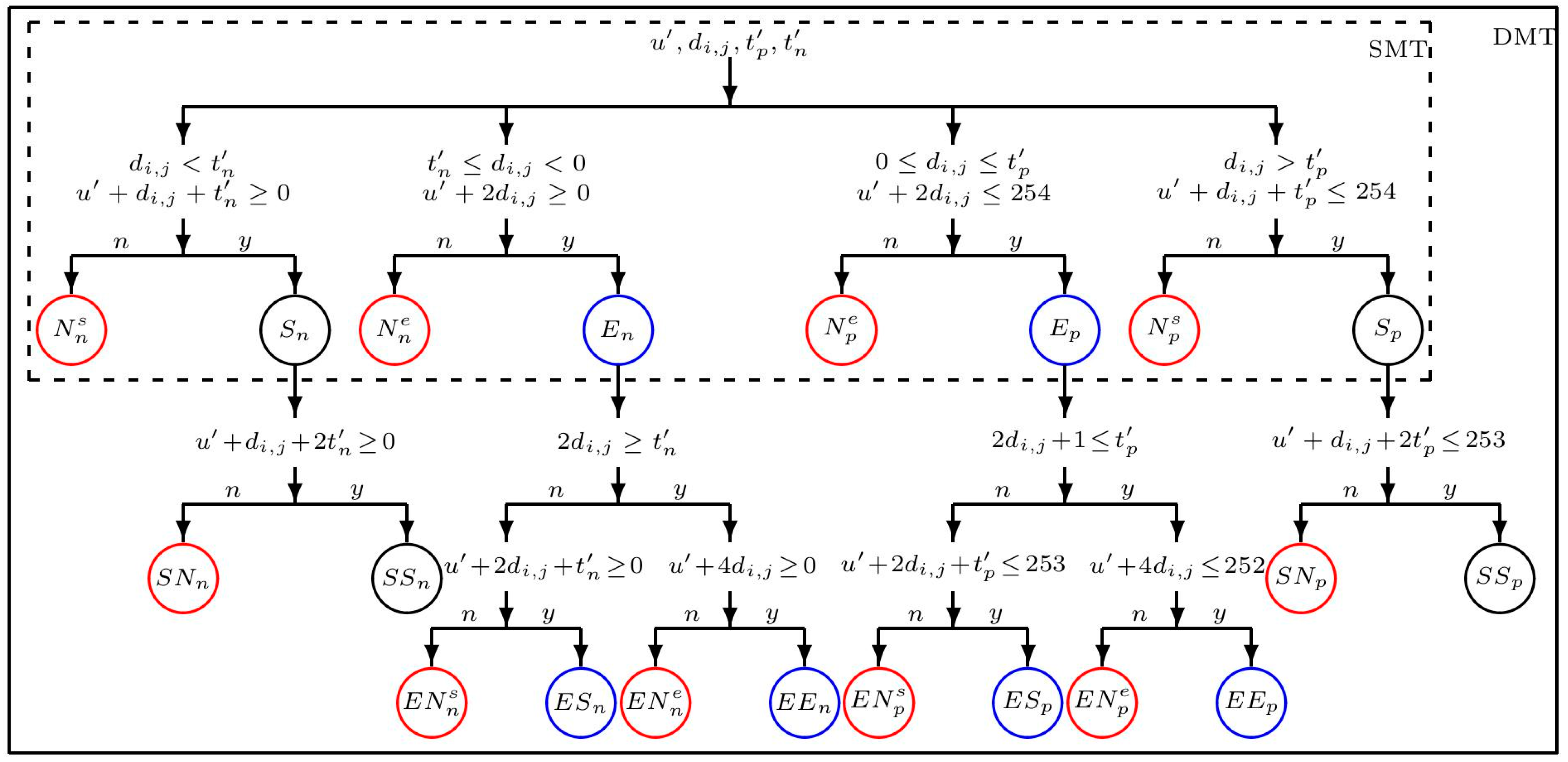
Figure 2. Flowchart of SMT and DMT sets. The eight sets of SMT are N^s_n, S_n, N^e_n, E_n, N^e_p, E_p, N^s_p, and S_p. The sixteen sets of DMT are N^s_n, SN_n, SS_n, N^e_n, EN^s_n, ES_n, EN^e_n, EE_n, N^e_p, EN^s_p, ES_p, EN^e_p, EE_p, N^s_p, SN_p, and SS_p. The non-carrying sets with the location map, non-carrying sets without the location map, and carrying sets are marked by the red, black, and blue circles, respectively.

3.2. The Supremum and Infimum for SMT

To begin, we separate the whole image pixels into sets of pixels which have the same predicted value, u′_i,j = u′. For each set of predicted value, we define eight sets of the SMT (see Figure 2) of pixels to which we will frequently refer to below. The parameters, t′_n, t′_p, and u′ are in the properties that are characteristic of all pixels in the sets:

$$E_n(t_n^{\prime })=\{(i,j):d_{i,j}\in [t_n^{\prime },0),u^{\prime }+2d_{i,j}\ge 0\},$$

$$S_n(t_n^{\prime })=\{(i,j):d_{i,j}\in [-u^{\prime },t_n^{\prime }),u^{\prime }+d_{i,j}+t_n^{\prime }\ge 0\},$$

$$N_n^e(t_n^{\prime })=\{(i,j):d_{i,j}\in [t_n^{\prime },0),u^{\prime }+2d_{i,j}<0\},$$

$$N_n^s(t_n^{\prime })=\{(i,j):d_{i,j}\in [-u^{\prime },t_n^{\prime }),u^{\prime }+d_{i,j}+t_n^{\prime }<0\},$$

$$E_p(t_p^{\prime })=\{(i,j):d_{i,j}\in [0,t_p^{\prime }],u^{\prime }+2d_{i,j}\le 254\},$$

$$S_p(t_p^{\prime })=\{(i,j):d_{i,j}\in (t_p^{\prime },255-u^{\prime }],u^{\prime }+d_{i,j}+t_p^{\prime }\le 254\},$$

$$N_p^e(t_p^{\prime })=\{(i,j):d_{i,j}\in [0,t_p^{\prime }],u^{\prime }+2d_{i,j}>254\},$$

$$N_p^s(t_p^{\prime })=\{(i,j):d_{i,j}\in (t_p^{\prime },255-u^{\prime }],u^{\prime }+d_{i,j}+t_p^{\prime }>254\},$$

E_n and E_p are the expandable sets. S_n and S_p are the shiftable sets. N^e_n and N^e_p are the unexpandable sets. N^s_n and N^s_p are the unshiftable sets. We should mention that N^e_n, N^e_p, N^s_n and N^s_p require the location map due to the overflow/underflow problem. In this section, we take N_n = N^e_n $\cup$ N^s_n and N_p = N^e_p $\cup$ N^s_p.

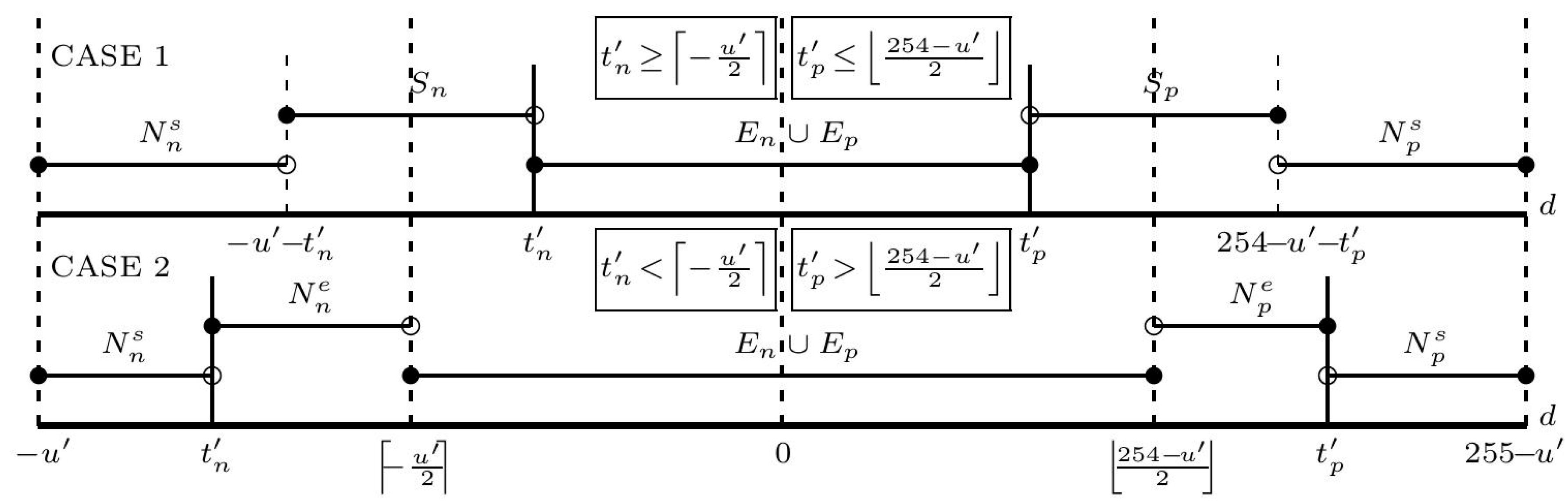
For simplicity in investigating the infimum of t′_n for each predicted value, we begin to separate the SMT sets (see Figure 3) into two cases as follows:

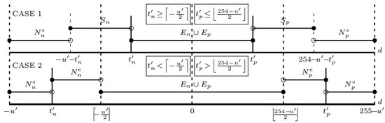
Figure 3. Two cases of separating SMT sets for investigating the supremun of t′_p and infimum of t′_n for each predicted value.

• Case 1: If $⌈-u^{\prime }/2⌉\le t_n^{\prime }\le 0$, here $u^{\prime }=2⌊u^{\prime }/2⌋+r$, where r $\in$ {0,1} is a remainder of u′ divided by 2, then $E_n(t_n^{\prime })\subseteq E_n(⌈-u^{\prime }/2⌉)$ and $N_n(t_n^{\prime })\subseteq N_n(⌈-u^{\prime }/2⌉);$

$$E_n(t_n^{\prime })=\{(i,j):d_{i,j}\in [t_n,0)\},$$

$$E_n(⌈-u^{\prime }/2⌉)=\{(i,j):d_{i,j}\in [⌈-u^{\prime }/2⌉,0)\},$$

$$S_n(t_n^{\prime })=\{(i,j):d_{i,j}\in [-u^{\prime }-t_n^{\prime },t_n^{\prime })\},$$

$$S_n(⌈-u^{\prime }/2⌉)=\{(i,j):d_{i,j}\in [⌈-u^{\prime }/2⌉-r,⌈-u^{\prime }/2⌉)\},$$

$$N_n^e(t_n^{\prime })=\varphi ,$$

$$N_n^s(t_n^{\prime })=\{(i,j):d_{i,j}\in [-u^{\prime },-u^{\prime }-t_n^{\prime })\},$$

$$N_n(t_n^{\prime })=\{(i,j):d_{i,j}\in [-u^{\prime },-u^{\prime }-t_n^{\prime })\},$$

$$N_n(⌈-u^{\prime }/2⌉)=\{(i,j):d_{i,j}\in [-u^{\prime },⌈-u^{\prime }/2⌉-r)\}.$$

Case 2: If $-u^{\prime }\le t_n^{\prime }<⌈-u^{\prime }/2⌉$, then $E_n(t_n^{\prime })=E_n(⌈-u^{\prime }/2⌉)$ and $N_n(t_n^{\prime })\supseteq N_n(⌈-u^{\prime }/2⌉);$

$$E_n(t_n^{\prime })=\{(i,j):d_{i,j}\in [⌈-u^{\prime }/2⌉,0)\},$$

$$S_n(t_n^{\prime })=\varphi ,$$

$$N_n^e(t_n^{\prime })=\{(i,j):d_{i,j}\in [t_n^{\prime },⌈-u^{\prime }/2⌉)\},$$

$$N_n^s(t_n^{\prime })=\{(i,j):d_{i,j}\in [-u^{\prime },t_n^{\prime })\},$$

$$N_n(t_n^{\prime })=\{(i,j):d_{i,j}\in [-u^{\prime },⌈-u^{\prime }/2⌉)\}.$$

$⌈.⌉$ and $⌊.⌋$ are the ceiling and floor functions. Notice that the largest expandable set is provided when t′_n is less than or equal to $⌈-u^{\prime }/2⌉$. Then, it is not necessary to reduce t′_n to be less than $⌈-u^{\prime }/2⌉$ because the reduction in t′_n increases the number of overflow/underflow pixels. The infimum of t′_n is $⌈-u^{\prime }/2⌉$ for each predicted value. We mention that the comparison of problematic sets between case 1 $(t_n^{\prime }=⌈-u^{\prime }/2⌉)$ and case 2 was clarified by plugging $u^{\prime }=2⌊u^{\prime }/2⌋+r$ into $N_n=(⌈-u^{\prime }/2⌉)$ for case 1. For example, if u′ = 5 then r = 1 (see Figure 1a). This means the pixels whose prediction-errors are −3 are prevented from becoming problematic pixels when we stop t′_n at −2. There are no preventable pixels when r = 0, because the problematic sets for case 1 $(t_n^{\prime }=⌈-u^{\prime }/2⌉)$ and case 2 are equal $(N_n=(⌈-u^{\prime }/2⌉)$= $N_n(t_n^{\prime }),t_n^{\prime }<⌈-u^{\prime }/2⌉)$.

For t′_p, the SMT sets are also separated into two cases (see Figure 3) and the supremum of t′_p will be investigated. The details are described as below:

• Case 1: If $0\le$ $t_p^{\prime }\le$ $⌊(254-u^{\prime })/2⌋$, here $254-u^{\prime }$ $=$ $2⌊(254-u^{\prime })/2⌋+r$, where r $\in$ {0,1} is a remainder of 254 − u’ divided by 2, then $E_p(t_p^{\prime })\supseteq E_p(⌊(254-u^{\prime })/2⌋)$ and $N_p(t_p^{\prime })\supseteq$ $N_p(⌊(254-u^{\prime })/2⌋);$

  $$E_p(t_p^{\prime })=\{(i,j):d_{i,j}\in [0,t_p^{\prime }]\},$$

  $$E_p(⌊(254-u^{\prime })/2⌋)=\{(i,j):d_{i,j}\in [0,⌊(254-u^{\prime })/2⌋]\},$$

$$S_p(t_p^{\prime })=\{(i,j):d_{i,j}\in (t_p^{\prime },254-u^{\prime }-t_p^{\prime }]\},$$

$$S_p(⌊(254-u^{\prime })/2⌋)=\{(i,j):d_{i,j}\in (⌊(254-u^{\prime })/2⌋,⌊(254-u^{\prime })/2⌋+r]\},$$

$$N_p^e(t_p^{\prime })=\varphi ,$$

$$N_p^s(t_p^{\prime })=\{(i,j):d_{i,j}\in (254-u^{\prime }-t_p^{\prime },255-u^{\prime }]\},$$

$$N_p(t_p^{\prime })=\{(i,j):d_{i,j}\in (254-u^{\prime }-t_p^{\prime },255-u^{\prime }]\},$$

$$N_p(⌊(254-u^{\prime })/2⌋)=\{(i,j):d_{i,j}\in (⌊(254-u^{\prime })/2⌋+r,255-u^{\prime }]\}.$$

Case 2: If $⌊(254-u^{\prime })/2⌋<t_p^{\prime }\le 255-u^{\prime }$, then $E_p(t_p^{\prime })=E_p(⌊(254-u^{\prime })/2⌋)$ and $N_p(t_p^{\prime })\supseteq$ $N_p(⌊(254-u^{\prime })/2⌋);$

$$E_p(t_p^{\prime })=\{(i,j):d_{i,j}\in [0,⌊(254-u^{\prime })/2⌋]\},$$

$$S_p(t_p^{\prime })=\varphi ,$$

$$N_p^e(t_p^{\prime })=\{(i,j):d_{i,j}\in (⌊(254-u^{\prime })/2⌋,t_p^{\prime }]\},$$

$$N_p^s(t_p^{\prime })=\{(i,j):d_{i,j}\in (t_p^{\prime },255-u^{\prime }]\},$$

$$N_p(t_p^{\prime })=\{(i,j):d_{i,j}\in (⌊(254-u^{\prime })/2⌋,255-u^{\prime }]\}.$$

Case 1 and 2 strongly prove that the supremum of t′_p is $⌊(254-u^{\prime })/2⌋$ for each predicted value (except for u′ = 255). Because the pixels whose predicted values and prediction errors equal 255 and 0 are always problematic pixels even when t′_p = 0, these pixels will never change. For instance, u′_i,j = 255 and d_i,j = 0 appear in some natural images (Tiffany, Kodim20 [52], etc.). We argue that the decoder does not err in these cases because these pixels are easily retrieved by calculating their predicted and prediction-error values.

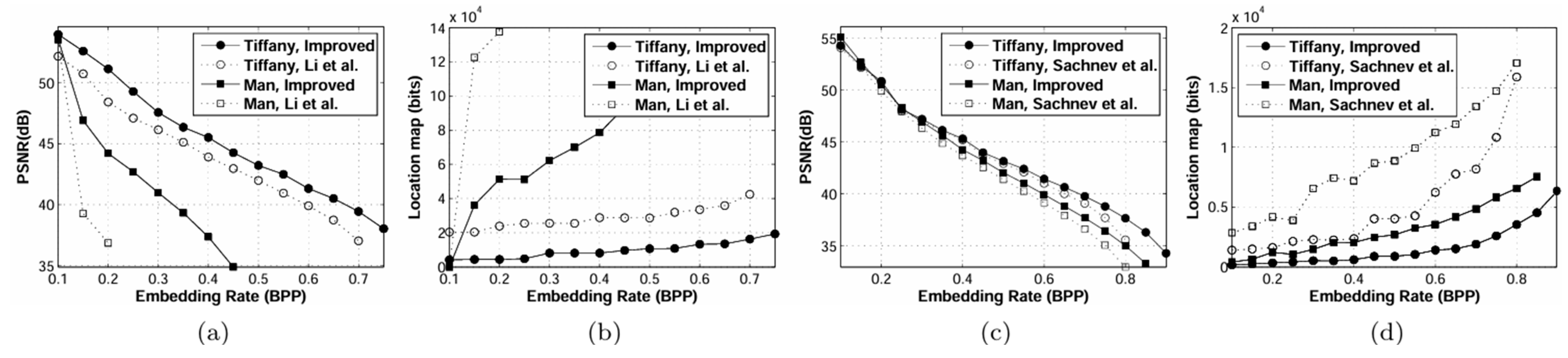
Following by the above strategy, we select t′_n and t′_p for the pixels, u′_i,j = u′, by t′_n = max{t_n, $⌈-u^{\prime }/2⌉$} and t′_p = min{t_p, $⌊(254-u^{\prime })/2⌋$}. t_n and t_p (global thresholds) are chosen; the cardinality of all expandable sets, $\left|{\cup }_{u\prime =0}^{255}(E_n(t_n^{\prime })\cup E_p(t_p^{\prime }))\right|,$ is large enough for all data bits to be embedded. For instance, t_n and t_p of the image are −3 and 2, respectively. Suppose now that we have u′ = 251 (see Figure 1b). t′_n = max{t_n, $⌈-u^{\prime }/2⌉$} = max{−3, $⌈-251/2⌉$} = −3 and t′_p = min{t_p, $⌊(254-u^{\prime })/2⌋$} = min{2, $⌊(254-251)/2⌋$} = 1 for this predicted value. In order to demonstrate the effectiveness of our proposal, we compare the results of our method with the method proposed by Li et al. [23]. Figure 4 depicts the rate-distortion curves of the original and improved versions of algorithm I [23], showing that restricting t′_n on [ $⌈-u^{\prime }/2⌉$, 0] and t′_p on [0, $⌊(254-u^{\prime })/2⌋$] can increase the peak signal-to-noise ratio (PSNR). In other words, the size of the location map is reduced. There are more spaces to embed the messages, hence a greater improvement of the PSNR. We should mention that their method still has one t_n and one t_p for the decoder.

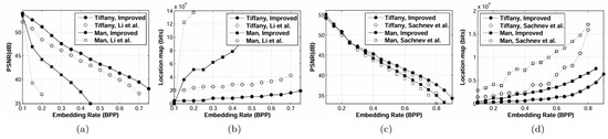
Figure 4. Comparison of embedding rate in BPP versus distortion in PSNR, (a,c), and location map in bits, (b,d), after improvement of Li et al.’s method [23], algorithm I, (a,b), and Sachnev et al.’s method [17], (c,d). The test images are Tiffany and Man.

3.3. The Supremum and Infimum for DMT

In simple terms, infimum represents the greatest possible lower bound, while supremum represents the smallest possible upper bound of a set. In order to simplify the explanation of our method for discovering the infimum of t′_n and the supremum of t′_p for DMT, we define other six sets of DMT for t′_n and other six sets of DMT for t′_p (see Figure 2). These sets can be written as follows:

$$E{E}_n(t_n^{\prime })=\{(i,j)\in E_n(t_n^{\prime }):2d_{i,j}\in [t_n^{\prime },0),u^{\prime }+4d_{i,j}\ge 0\},$$

$$E{S}_n(t_n^{\prime })=\{(i,j)\in E_n(t_n^{\prime }):2d_{i,j}\in [2t_n^{\prime },t_n^{\prime }),u^{\prime }+2d_{i,j}+t_n^{\prime }\ge 0\},$$

$$E{N}_n^e(t_n^{\prime })=\{(i,j)\in E_n(t_n^{\prime }):2d_{i,j}\in [t_n^{\prime },0),u^{\prime }+4d_{i,j}<0\},$$

$$E{N}_n^s(t_n^{\prime })=\{(i,j)\in E_n(t_n^{\prime }):2d_{i,j}\in [2t_n^{\prime },t_n^{\prime }),u^{\prime }+2d_{i,j}+t_n^{\prime }<0\},$$

$$S{S}_n(t_n^{\prime })=\{(i,j)\in S_n(t_n^{\prime }):u^{\prime }+d_{i,j}+2t_n^{\prime }\ge 0\},$$

$$S{N}_n(t_n^{\prime })=\{(i,j)\in S_n(t_n^{\prime }):u^{\prime }+d_{i,j}+2t_n^{\prime }<0\},$$

$$E{E}_p(t_p^{\prime })=\{(i,j)\in E_p(t_p^{\prime }):2d_{i,j}\in [0,t_p^{\prime }-1],u^{\prime }+4d_{i,j}\le 252\},$$

$$E{S}_p(t_p^{\prime })=\{(i,j)\in E_p(t_p^{\prime }):2d_{i,j}\in (t_p^{\prime }-1,2t_p^{\prime }],u^{\prime }+2d_{i,j}+t_p^{\prime }\le 253\},$$

$$E{N}_p^e(t_p^{\prime })=\{(i,j)\in E_p(t_p^{\prime }):2d_{i,j}\in [0,t_p^{\prime }-1],u^{\prime }+4d_{i,j}>252\},$$

$$E{N}_p^s(t_p^{\prime })=\{(i,j)\in E_p(t_p^{\prime }):2d_{i,j}\in (t_p^{\prime }-1,2t_p^{\prime }],u^{\prime }+2d_{i,j}+t_p^{\prime }>253\},$$

$$S{S}_p(t_p^{\prime })=\{(i,j)\in S_p(t_p^{\prime }):u^{\prime }+d_{i,j}+2t_p^{\prime }\le 253\},$$

$$S{N}_p(t_p^{\prime })=\{(i,j)\in S_p(t_p^{\prime }):u^{\prime }+d_{i,j}+2t_p^{\prime }>253\},$$

These twelve sets are named from their elements’ behavior. E, S and N are abbreviated from expandable, shiftable, and non expanable-shiftable. The first and second letters represent the first and second modifications of pixels. For example, ES_n is a set of pixels whose negative prediction-error is expanded in the first and shifted in the second without an underflow problem. The pixels of EE_n, EE_p, ES_n, and ES_p are embedded the message and the prediction-error of pixels in SS_n and SS_p are shifted without conveying any data. EN^e_n, EN^e_p, EN^s_n, EN^s_p, SN^s_n and SN^s_p are the problematic sets. The prediction-errors of the pixels of SN^s_n and SN^s_p are shifted and the prediction-errors of pixels of EN^e_n, EN^e_p, EN^s_n, and EN^s_p need to be expanded once and added to the extreme bit value to ensure reversibility. Sachnev et al. [17] provide a detailed analysis of various cases, including both problematic and non-problematic pixels, in their study. For simplicity in this section we take M_n = EN^e_n $\cup$ EN^s_n $\cup$ N^e_n $\cup$ SN_n $\cup$ N^s_n, M_p = EN^e_p $\cup$ EN^s_p $\cup$ N^e_p $\cup$ SN_p $\cup$ N^s_p, C_n = EE_n $\cup$ ES_n, and C_p = EE_p $\cup$ ES_p.

Restricting t′_n and t′_p to their infimum and supremum, respectively, ensures the maximum number of embeddable pixels with the smallest possible location map (refer to Figure 1). The analysis of the DMT sets is divided into three cases, as shown in Figure 5:

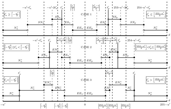
Figure 5. Three cases of separating DMT sets for investigating the infimum of t′_n and supremun of t′_p for each predicted value.

• Case 1: If $⌈-u^{\prime }/3⌉\le t_n^{\prime }\le 0$, here $u^{\prime }=3⌊u^{\prime }/3⌋+r$, where r $\in${0,1,2} is a remainder of u′ divided by 3, then $C_n(t_n^{\prime })\subseteq C_n(⌈-u^{\prime }/3⌉)$ and $M_n(t_n^{\prime })\subseteq M_n(⌈-u^{\prime }/3⌉);$

$$E{E}_n(t_n^{\prime })=\{(i,j):d_{i,j}\in [⌈t_n^{\prime }/2⌉,0)\},$$

$$E{S}_n(t_n^{\prime })=\{(i,j):d_{i,j}\in [t_n^{\prime },⌈t_n^{\prime }/2⌉)\},$$

$$C_n(t_n^{\prime })=\{(i,j):d_{i,j}\in [t_n^{\prime },0)\},$$

$$C_n(⌈-u^{\prime }/3⌉)=\{(i,j):d_{i,j}\in [⌈-u^{\prime }/3⌉,0)\},$$

$$S{S}_n(t_n^{\prime })=\{(i,j):d_{i,j}\in [-u^{\prime }-2t_n^{\prime },t_n^{\prime })\},$$

$$S{S}_n(⌈-u^{\prime }/3⌉)=\{(i,j):d_{i,j}\in [⌈-u^{\prime }/3⌉-r,⌈-u^{\prime }/3⌉)\},$$

$$E{N}_n^e(t_n^{\prime })=E{N}_n^s(t_n^{\prime })=N_n^e(t_n^{\prime })=\varphi ,$$

$$S{N}_n(t_n^{\prime })=\{(i,j):d_{i,j}\in [-u^{\prime }-t_n^{\prime },-u^{\prime }-2t_n^{\prime })\},$$

$$N_n^s(t_n^{\prime })=\{(i,j):d_{i,j}\in [-u^{\prime },-u^{\prime }-t_n^{\prime })\},$$

$$M_n(t_n^{\prime })=\{(i,j):d_{i,j}\in [-u^{\prime },-u^{\prime }-2t_n^{\prime })\},$$

$$M_n(⌈-u^{\prime }/3⌉)=\{(i,j):d_{i,j}\in [-u^{\prime },⌈-u^{\prime }/3⌉-r)\}.$$

Case 2: If $⌈-u^{\prime }/2⌉\le t_n^{\prime }<⌈-u^{\prime }/3⌉$, here $t_n^{\prime }=⌈-u^{\prime }/3⌉-\gamma$, where $\gamma =1,\dots ,$ $⌈-u^{\prime }/3⌉-$ $⌈-u^{\prime }/2⌉$, then $C_n(t_n^{\prime })\subseteq C_n(⌈-u^{\prime }/3⌉)$ and $M_n(t_n^{\prime })\supseteq M_n(⌈-u^{\prime }/3⌉);$

$$E{E}_n(t_n^{\prime })=\{(i,j):d_{i,j}\in [⌈t_n^{\prime }/2⌉,0)\},$$

$$E{S}_n(t_n^{\prime })=\{(i,j):d_{i,j}\in [⌈(-u^{\prime }-t_n^{\prime })/2⌉,⌈t_n^{\prime }/2⌉)\},$$

$$C_n(t_n^{\prime })=\{(i,j):d_{i,j}\in [⌈(-u^{\prime }-t_n^{\prime })/2⌉,0)\},$$

$$C_n(⌈-u^{\prime }/3⌉-\gamma )=\{(i,j):d_{i,j}\in [⌈-u^{\prime }/3⌉+⌈(\gamma -r)/2⌉,0)\},$$

$$S{S}_n(t_n^{\prime })=\varphi ,$$

$$E{N}_n^e(t_n^{\prime })=N_n^e(t_n^{\prime })=\varphi ,$$

$$E{N}_n^s(t_n^{\prime })=\{(i,j):d_{i,j}\in [t_n^{\prime },⌈(-u^{\prime }-t_n^{\prime })/2⌉)\},$$

$$S{N}_n(t_n^{\prime })=\{(i,j):d_{i,j}\in [-u^{\prime }-t_n^{\prime },t_n^{\prime })\},$$

$$N_n^s(t_n^{\prime })=\{(i,j):d_{i,j}\in [-u^{\prime },-u^{\prime }-t_n^{\prime })\},$$

$$M_n(t_n^{\prime })=\{(i,j):d_{i,j}\in [-u^{\prime },⌈(-u^{\prime }-t_n^{\prime })/2⌉)\},$$

$$M_n(⌈-u^{\prime }/3⌉-\gamma )=\{(i,j):d_{i,j}\in [-u^{\prime },⌈-u^{\prime }/3⌉+⌈(\gamma -r)/2⌉)\}.$$

Case 3: If $-u^{\prime }\le t_n^{\prime }<⌈-u^{\prime }/2⌉$, then $C_n(t_n^{\prime })\subseteq C_n(⌈-u^{\prime }/3⌉)$ and $M_n(t_n^{\prime })\supseteq M_n(⌈-u^{\prime }/3⌉);$

$$E{E}_n(t_n^{\prime })=\{(i,j):d_{i,j}\in [⌈-u^{\prime }/4⌉,0)\},$$

$$E{S}_n(t_n^{\prime })=\varphi ,$$

$$C_n(t_n^{\prime })=\{(i,j):d_{i,j}\in [⌈-u^{\prime }/4⌉,0)\},$$

$$S{S}_n(t_n^{\prime })=\varphi ,$$

$$E{N}_n^e(t_n^{\prime })=\{(i,j):d_{i,j}\in [⌈t_n^{\prime }/2⌉,⌈-u^{\prime }/4⌉)\},$$

$$E{N}_n^s(t_n^{\prime })=\{(i,j):d_{i,j}\in [⌈-u^{\prime }/2⌉,⌈t_n^{\prime }/2⌉)\},$$

$$N_n^e(t_n^{\prime })=\{(i,j):d_{i,j}\in [t_n^{\prime },⌈-u^{\prime }/2⌉)\},$$

$$S{N}_n^s(t_n^{\prime })=\varphi ,$$

$$N_n^s(t_n^{\prime })=\{(i,j):d_{i,j}\in [-u^{\prime },t_n^{\prime })\},$$

$$M_n(t_n^{\prime })=\{(i,j):d_{i,j}\in [-u^{\prime },⌈-u^{\prime }/4⌉)\},$$

We can see that $C_n(t_n^{\prime })\subseteq C_n(⌈-u^{\prime }/3⌉)$ and $M_n(t_n^{\prime })\supseteq M_n(⌈-u^{\prime }/3⌉);$ for $t_n^{\prime }\in [-u^{\prime },$ $⌈-u^{\prime }/3⌉)$. This implies that the infimum of t′_n for DMT is $⌈-u^{\prime }/3⌉$. Let us consider the details in each case. In case 3, even if t′_n is decreased, C_n and M_n are completely frozen and the number of underflow pixels is the largest of all cases; meanwhile, the number of embeddable pixels is smaller than or equal to the largest possible number in case 1 and 2. In case 2, the number of embeddable pixels is reduced, while the number of underflow pixels is increased when t′_n is decreased. Finally, in case 1, both sets are enlarged, as t′_n is decreased there is more space to convey the data and the number of problematic pixels is increased. Figure 4 shows that the location map graphs give strong supporting evidence for this claim. For some u′, the largest embeddable sets for all cases are identical, but the corresponding problematic set of case 1 is actually different from case 2 and 3. u′ = 5 is one example (see Figure 6). The largest C_n(t′_n) of all cases is {(i,j): d_i,j $\in$[−1, 0)}:

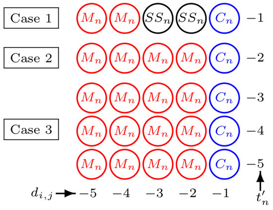
Figure 6. Example on case 1, 2, and 3 of u’ = 5 for DMT.

• Case 1: $C_n(t_n^{\prime })=\{(i,j):d_{i,j}\in [⌈-u^{\prime }/3⌉,0)\}$ for $t_n^{\prime }=$ $⌈-u^{\prime }/3⌉$,
• Case 2: $C_n(t_n^{\prime })=\{(i,j):d_{i,j}\in [⌈-u^{\prime }/3⌉+⌈(\gamma -r)/2⌉,0)\}$ for $t_n^{\prime }=⌈-u^{\prime }/3⌉-\gamma ,$ $r=u^{\prime }$ $-3⌊u^{\prime }/3⌋=2,$
• Case 3: If $C_n(t_n^{\prime })=\{(i,j):d_{i,j}\in [⌈-u^{\prime }/4⌉,0)\}.$

$M_n(⌈-u^{\prime }/3⌉)$ of case 1 is smaller than $M_n(⌈-u^{\prime }/3⌉-\gamma )$ of case 2 and M_n(t′_n) of case 3:

• Case 1: $M_n(⌈-u^{\prime }/3⌉)=\{(i,j):d_{i,j}\in [-u^{\prime },⌈-u^{\prime }/3⌉-r)\}=\{(i,j):d_{i,j}\in [-5,-3)\}$
• Case 2: $M_n(⌈-u^{\prime }/3⌉-\gamma )=\{(i,j):d_{i,j}\in [-u^{\prime },⌈-u^{\prime }/3⌉+⌈(\gamma -r)/2⌉)\}=\{(i,j):$ $d_{i,j}\in [-5,-1)\}$
• Case 3: If $M_n(t_n^{\prime })=\{(i,j):d_{i,j}\in [-u^{\prime },⌈-u^{\prime }/4⌉)\}=\{(i,j):d_{i,j}\in [-5,-1)\}$

Finally, we investigate further the supremum of t′_p for DMT as follows:

• Case 1: If $0\le t_p^{\prime }\le ⌊(253-u^{\prime })/3⌋$, here $253-u^{\prime }=$ $3⌊(253-u^{\prime })/3⌋+r$, where r $\in${0,1,2} is a remainder of 253 − u’ divided by 3, then $C_p(t_p^{\prime })\subseteq C_p(⌊(253-u^{\prime })/3⌋)$ and $M_p(t_p^{\prime })\supseteq$ $M_p(⌊(253-u^{\prime })/3⌋);$

$$E{E}_p(t_p^{\prime })=\{(i,j):d_{i,j}\in [0,⌊(t_p^{\prime }-1)/2⌋]\},$$

$$E{S}_p(t_p^{\prime })=\{(i,j):d_{i,j}\in [⌊(t_p^{\prime }-1)/2⌋,t_p^{\prime }]\},$$

$$C_p(t_p^{\prime })=\{(i,j):d_{i,j}\in [0,t_p^{\prime }]\},$$

$$C_p(⌊(253-u^{\prime })/3⌋)=\{(i,j):d_{i,j}\in [0,⌊(253-u^{\prime })/3⌋]\},$$

$$S{S}_p(t_p^{\prime })=\{(i,j):d_{i,j}\in (t_p^{\prime },253-u^{\prime }-2t_p^{\prime }]\},$$

$$S{S}_p(⌊(253-u^{\prime })/3⌋)=\{(i,j):d_{i,j}\in (⌊(253-u^{\prime })/3⌋,⌊(253-u^{\prime })/3⌋+r]\},$$

$$E{N}_p^e(t_p^{\prime })=E{N}_p^s(t_p^{\prime })=N_p^e(t_p^{\prime })=\varphi ,$$

$$S{N}_p(t_p^{\prime })=\{(i,j):d_{i,j}\in (253-u^{\prime }-2t_p^{\prime },254-u^{\prime }-t_p^{\prime }]\},$$

$$N_p^s(t_p^{\prime })=\{(i,j):d_{i,j}\in (254-u^{\prime }-t_p^{\prime },255-u^{\prime })\},$$

$$M_p(t_p^{\prime })=\{(i,j):d_{i,j}\in (253-u^{\prime }-2t_p^{\prime },255-u^{\prime }]\},$$

$$M_n(⌊(253-u^{\prime })/3⌋)=\{(i,j):d_{i,j}\in (⌊(253-u^{\prime })/3⌋+r,255-u^{\prime }]\}.$$

Case 2: If $⌊(253-u^{\prime })/3⌋<t_p^{\prime }\le ⌊(254-u^{\prime })/2⌋$, here $t_p^{\prime }=⌊253-u^{\prime })/3⌋+\gamma$, where $\gamma =1,\dots ,⌊254-u^{\prime })/2⌋-$ $⌊253-u^{\prime })/3⌋,$ then $C_p(t_p^{\prime })\subseteq C_p(⌊(253-u^{\prime })/3⌋)$ and $M_p(t_p^{\prime })\supseteq$ $M_p(⌊(253-u^{\prime })/3⌋);$

$$E{E}_p(t_p^{\prime })=\{(i,j):d_{i,j}\in [0,⌊(t_p^{\prime }-1)/2⌋]\},$$

$$E{S}_p(t_p^{\prime })=\{(i,j):d_{i,j}\in [⌊(t_p^{\prime }-1)/2⌋,⌊(253-u^{\prime }-t_p^{\prime })/2⌋]\},$$

$$C_p(t_p^{\prime })=\{(i,j):d_{i,j}\in [0,⌊(253-u^{\prime }-t_p^{\prime })/2⌋]\},$$

$$C_p(⌊(253-u^{\prime })/3⌋+\gamma )=\{(i,j):d_{i,j}\in [0,⌊(253-u^{\prime })/3⌋+⌊(r-\gamma )/2⌋]\},$$

$$S{S}_p(t_p^{\prime })=\varphi ,$$

$$E{N}_p^e(t_p^{\prime })=N_p^s(t_p^{\prime })=\varphi ,$$

$$E{N}_p^s(t_p^{\prime })=\{(i,j):d_{i,j}\in (⌊(253-u^{\prime }-t_p^{\prime })/2⌋,t_p^{\prime }]\},$$

$$S{N}_p(t_p^{\prime })=\{(i,j):d_{i,j}\in (t_p^{\prime },254-u^{\prime }-t_p^{\prime }]\},$$

$$N_p^s(t_p^{\prime })=\{(i,j):d_{i,j}\in (254-u^{\prime }-t_p^{\prime },255-u^{\prime }]\},$$

$$M_p(t_p^{\prime })=\{(i,j):d_{i,j}\in (⌊253-u^{\prime }-t_p^{\prime }⌋,255-u^{\prime }]\},$$

$$M_p(⌊(253-u^{\prime })/3⌋+\gamma )=\{(i,j):d_{i,j}\in (⌊(253-u^{\prime })/3⌋+⌊(r-\gamma )/2⌋,255-u^{\prime }]\}.$$

Case 3: If $⌊(254-u^{\prime })/2⌋\le t_p^{\prime }\le 255-u^{\prime }$, then $C_p(t_p^{\prime })\subseteq C_p(⌊(253-u^{\prime })/3⌋)$ and $M_p(t_p^{\prime })\supseteq$ $M_p(⌊(253-u^{\prime })/3⌋);$

$$E{E}_p(t_p^{\prime })=\{(i,j):d_{i,j}\in [0,⌊(252-u^{\prime })/4⌋]\},$$

$$E{S}_p(t_p^{\prime })=\varphi ,$$

$$C_p(t_p^{\prime })=\{(i,j):d_{i,j}\in [0,⌊(252-u^{\prime })/4⌋]\},$$

$$S{S}_p(t_p^{\prime })=\varphi ,$$

$$E{N}_p^e(t_p^{\prime })=\{(i,j):d_{i,j}\in (⌊(252-u^{\prime })/4⌋,⌊(t_p^{\prime }-1)/2⌋]\},$$

$$E{N}_p^s(t_p^{\prime })=\{(i,j):d_{i,j}\in (⌊(t_p^{\prime }-1)/2⌋,⌊(254-u^{\prime })/2⌋]\},$$

$$N_p^e(t_p^{\prime })=\{(i,j):d_{i,j}\in (⌊(254-u^{\prime })/2⌋,t_p^{\prime }]\},$$

$$S{N}_p(t_p^{\prime })=\varphi ,$$

$$N_p^s(t_p^{\prime })=\{(i,j):d_{i,j}\in (t_p^{\prime },255-u^{\prime }]\},$$

$$M_p(t_p^{\prime })=\{(i,j):d_{i,j}\in (⌊(252-u^{\prime })/4⌋,255-u^{\prime }]\}.$$

Referring to all cases above, the supremum of t′_p is $⌊(253-u^{\prime })/3⌋$. Note that the pixels with predicted values of 254 or 255 and non-negative prediction-errors (d_i,j $\ge$ 0) are not utilized in the embedding scheme because they cannot be embedded the data even when t′_p = 0. Thus, it is unnecessary to mark them onto the location map. Extraction is performed by calculating their prediction-errors and predicted values.

Following by the above strategy, we select t′_n and t′_p for the pixels, u′_i,j = u′, by t′_n = max{t_n, $⌈(-u^{\prime }/3)⌉$} and t′_p = min{t_p, $⌊(253-u^{\prime })/3⌋$}. t_n and t_p (global thresholds) are chosen; $\left|{\cup }_{u\prime =0}^{255}(C_n(t_n^{\prime })\cup C_p(t_p^{\prime }))\right|$ is large enough for all data bits to be embedded. For instance, t_n and t_p of the image are −3 and 2, respectively. Suppose now that we have u′ = 251 (see Figure 1d). t′_n = max{t_n, $⌈(-u^{\prime }/3)⌉$} = max{−3, $⌈(-251/3)⌉$} = −3 and t′_n= min{t_p, $⌈(-251/3)⌉$}= min{2, $⌊(253-251)/3⌋$} = 0 for this predicted value. In order to demonstrate the effectiveness of our scheme, we utilized our improvement on Sachnev et al.’s method [17] and the superior results obtained are depicted in Figure 4. For the entire embedding rate range, especially at high embedding rates, our improvement to the method of Sachnev et al. [17] clearly outperforms the original one. The improvement came from restricting t′_n on [ $⌈(-u^{\prime }/3)⌉$, 0] and t′_p on [0, $⌊(253-u^{\prime })/3⌋$]. Sachnev et al.’s method still has one t_n and one t_p for sending to the decoder. Stopping t′_n and t′_p at its infimum and supremum is very significant for RDH based on PEE and HS.

4. Advantage of the Supremum and Infimum

Now we can apply our newfound knowledge of the supremum and infimum to conclude our discussion on how to determine the first operating threshold and the formulas for decoding and encoding. Basically, PEE and HS combine to form an effective method for RDH, and these techniques need to determine the global thresholds (t_n and t_p) in order to achieve the lowest possible distortion. However, t′_n and t′_p should be restricted to [ $⌈(-u^{\prime }/3)⌉$, 0] and [0, $⌊(253-u^{\prime })/3⌋$] (case 1 of DMT). We will formulate the set of expandable, E(t_n, t_p), shiftable, S(t_n, t_p), and problematic pixels, M(t_n, t_p), which can be used for all predicted values. These sets are shown as follows:

$$E(t_n,t_p)={\cup }_{u\prime =0}^{255}[C_n({t^{\prime }}_n)\cup C_p({t^{\prime }}_p)]={\cup }_{u\prime =0}^{255}[C_n(max\{t_n,⌈-u^{\prime }/3⌉\})\cup C_p(min\{t_p,⌊(253-u^{\prime })/3⌋\})].$$

$$={\cup }_{u\prime =0}^{255}[\{(i,j):d_{i,j}\in [max\{t_n,⌈-u^{\prime }/3⌉\},min\{t_p,⌊(253-u^{\prime })/3⌋$$

$$={\cup }_{u\prime =0}^{255}[\{(i,j):d_{i,j}\in [t_n,t_p]\cap ⌈-u^{\prime }/3⌉,⌊(253-u^{\prime })/3⌋]\}].$$

$$=\{(i,j):d_{i,j}\in \underset{¯}{[t_n,t_p]}\cap \underset{¯}{⌈-u^{\prime }/3⌉,⌊(253-u^{\prime })/3⌋]}\}.$$

$$M(t_n,t_p)={\cup }_{u\prime =0}^{255}[M_n(max\{t_n,⌈-u^{\prime }/3⌉\})\cup M_p(min\{t_p,⌊(253-u^{\prime })/3⌋\})].$$

$$=\{(i,j):d_{i,j}\in (\underset{¯}{\underset{¯}{[-u_{i,j}^{\prime },-u_{i,j}^{\prime }-2t_n)}\cap \underset{¯}{[-u_{i,j}^{\prime },-u_{i,j}^{\prime }-2⌈-u_{i,j}^{\prime }/3⌉)}})\cup$$

$$(\underset{¯}{\underset{¯}{(253-u_{i,j}^{\prime }-2t_p,255-u_{i,j}^{\prime }]}\cap \underset{¯}{(253-u_{i,j}^{\prime }-2⌊(253-u_{i,j}^{\prime })/3⌋,255-u_{i,j}^{\prime }]}})\}.$$

$$S(t_n,t_p)={\cup }_{u\prime =0}^{255}[S{S}_n(max\{t_n,⌈-u^{\prime }/3⌉\})\cup S{S}_p(min\{t_p,⌊(253-u^{\prime })/3⌋\})].$$

$$=\{(i,j):d_{i,j}\in (\underset{¯}{\underset{¯}{[-u_{i,j}^{\prime }-2t_n,-t_n)}\cup \underset{¯}{[-u_{i,j}^{\prime }-2⌈-u_{i,j}^{\prime }/3⌉,⌈-u_{i,j}^{\prime }/3⌉)}})\cup$$

$$(\underset{¯}{\underset{¯}{(t_p,253-u_{i,j}^{\prime }-2t_p]}\cup \underset{¯}{(⌊(253-u_{i,j}^{\prime })/3⌋,253-u_{i,j}^{\prime }-2⌊(253-u_{i,j}^{\prime })/3⌋]}})\}.$$

4.1. Determining the First Operating Threshold

The first operating threshold should have the smallest distance between t_n and t_p carefully chosen so that the selected bins of the histogram of prediction-errors is at least as large as the total size of the payload, the location map, and the footer. The bit-stream of the location map is formed by collecting the problematic pixels whose sizes depend on t_n and t_p. Consequently, a measure of the frequency of the prediction error of histogram bins cannot be used to determine the first operating threshold.

We know that u′_i,j is a member of the set {0,…,255}. Among the basic properties of these sets are E(t_n, t_p) $\subseteq$ E(−85, 84), S(t_n, t_p) $\subseteq$ S(0, 0), and M(t_n, t_p) $\subseteq$ M(−85, 84). It is unnecessary to increase t_p to be greater than 84 and also to decrease t_n to be lower than −85. In addition, E(−85, 84) $\cap$ M(t_n, t_p) = $\varphi$. Heuristically, this means that both are disjointed for all t_n and t_p. In other words, they have no elements in common. We used this simple property to construct our strategy for finding the first operating threshold. Note that our scheme has continued to use the combination of the two paths: t_p + t_n = −1 and t_p + t_n = 0 [16,23], where t_n = − $⌊t/2⌋$, t_p = $⌈t/2⌉$ − 1 and t $\in${1,…,170} to determine the appropriate threshold. Algorithm 1 shows our recursive procedure for computing the first operating threshold. ne and nm are parameters to count the number of expandable and problematic pixels. Array A can be utilized to mark pixels which are members of the expandable and problematic set because the pixels are elements of those sets permanently: E(1) $\subseteq$ E(2) $\subseteq$… $\subseteq$ E(170), M(1) $\subseteq$ M(2) $\subseteq$… $\subseteq$ M(170), and E(170) $\cap$ M(t) = $\varphi$, $\forall t$. N is the number of pixels. The first iteration of the procedure is initialized by setting the threshold to its minimum value, t = 1(t_n = 0, t_p = 0). The process is repeated until either the number of expandable pixels equals the total size of the problematic pixels, the payload P and the footer Q or t equals 170. We assume that the first operating threshold is t_f. In the extreme case, there are N.t_f inspections by checking the property of E(t) and M(t). However, there are N.t_f − ${\displaystyle {\sum }_{t=1}^{t_f-1}(\left|E(t)\right|+\left|M(t)\right|)}$ inspections for this procedure. It should be more efficient (especially when the payload is high) even though there is an extra parameter A in the procedure.

Algorithm 1 The algorithm to determine the first operating threshold.

Comment: Array A is initialized with zero values. t = 0, ne = 0, nm = 0 while ne < nm + P + Q and t < 170 do ne = 0, nm = 0, k = 0, t = t + 1 $t_n=-⌊t/2⌋$$, t_p=⌈t/2⌉-1$ while ne < nm + P + Q and k < N do k = k + 1 if A(k) = 1 then ne = ne + 1 else if A(k) = 2 then nm = nm + 1 else if d(k) < 0 and tn $\ge$ − u′(k)/3 then if d(k) $\ge$ tn then ne = ne +1, A(k) = 1 else if d(k) < −u′(k) − 2tn then nm = nm + 1, A(k) = 2 end if else if d(k) $\ge$ 0 and tp $\le$ (253 − u′(k))/3 then if d(k) $\le$ tp then ne = ne + 1, A(k) = 1 else if d(k) > 253 − u′(k) − 2tp then nm = nm + 1, A(k) = 2 end if end if end while end while if ne = = nm + P + Q then tf = t end if

4.2. The Formulas for Decoding and Encoding

Either SMT or DMT can be combined with Formula (1) to identify pixels which require a location map. The advantage of using the three sets E(t_n, t_p), M(t_n, t_p), and S(t_n, t_p) in advance is that we can develop the formula for RDH based on PEE and HS algorithm without modification testing, and it can be defined as follows:

$$U_{i,j}=\left\{\begin{array}{c}{u}_{i,j}\begin{array}{c}\end{array}\begin{array}{c}\end{array}\begin{array}{c}\end{array}\begin{array}{c}\end{array}\begin{array}{c}\end{array}\begin{array}{c}\end{array}\begin{array}{c}\end{array}\begin{array}{c}\end{array}\begin{array}{c}\end{array}\hfill \\ u_{i,j}+t_p^{\prime }+1\begin{array}{c}\end{array}\begin{array}{c}\end{array}\begin{array}{c}\end{array}\begin{array}{c}\end{array}\hfill \\ u_{i,j}+t_p^{\prime }+1\begin{array}{c}\end{array}\begin{array}{c}\end{array}\begin{array}{c}\end{array}\begin{array}{c}\end{array}\hfill \\ u_{i,j}+d_{i,j}+b\begin{array}{c}\end{array}\begin{array}{c}\end{array}\begin{array}{c}\end{array}\hfill \\ u_{i,j}+t_n^{\prime }\begin{array}{c}\end{array}\begin{array}{c}\end{array}\begin{array}{c}\begin{array}{c}\end{array}\end{array}\begin{array}{c}\end{array}\begin{array}{c}\end{array}\begin{array}{c}\end{array}\hfill \\ u_{i,j}+t_n^{\prime }\begin{array}{c}\end{array}\begin{array}{c}\end{array}\begin{array}{c}\end{array}\begin{array}{c}\end{array}\begin{array}{c}\end{array}\begin{array}{c}\end{array}\hfill \\ u_{i,j}\begin{array}{c}\end{array}\begin{array}{c}\end{array}\begin{array}{c}\end{array}\begin{array}{c}\end{array}\begin{array}{c}\end{array}\begin{array}{c}\end{array}\begin{array}{c}\end{array}\begin{array}{c}\end{array}\begin{array}{c}\end{array}\hfill \end{array}\begin{array}{c}if\begin{array}{c}\end{array}{d}_{i,j}\in (254-u_{i,j}^{\prime }-t_p^{\prime },255-u_{i,j}^{\prime }]\begin{array}{c}\end{array}\begin{array}{c}\end{array}\begin{array}{c}\end{array}\begin{array}{c}\begin{array}{c}\end{array}\end{array}\hfill \\ if\begin{array}{c}\end{array}{d}_{i,j}\in (253-u_{i,j}^{\prime }-2t_p^{\prime },254-u_{i,j}^{\prime }-t_p^{\prime }]\hfill \\ if\begin{array}{c}\end{array}{d}_{i,j}\in (t_p^{\prime },253-u_{i,j}^{\prime }-2t_p^{\prime }]\begin{array}{c}\end{array}\begin{array}{c}\end{array}\begin{array}{c}\end{array}\begin{array}{c}\end{array}\begin{array}{c}\end{array}\begin{array}{c}\end{array}\begin{array}{c}\end{array}\begin{array}{c}\end{array}\hfill \\ if\begin{array}{c}\end{array}{d}_{i,j}\in [t_n^{\prime },t_p^{\prime }]\begin{array}{c}\end{array}\begin{array}{c}\end{array}\begin{array}{c}\end{array}\begin{array}{c}\end{array}\begin{array}{c}\begin{array}{c}\end{array}\begin{array}{c}\end{array}\begin{array}{c}\end{array}\begin{array}{c}\end{array}\begin{array}{c}\end{array}\begin{array}{c}\end{array}\begin{array}{c}\end{array}\begin{array}{c}\end{array}\begin{array}{c}\end{array}\begin{array}{c}\end{array}\begin{array}{c}\end{array}\begin{array}{c}\end{array}\begin{array}{c}\end{array}\end{array}\hfill \\ if\begin{array}{c}\end{array}{d}_{i,j}\in [-u_{i,j}^{\prime }-2t_n^{\prime },t_n^{\prime })\begin{array}{c}\end{array}\begin{array}{c}\end{array}\begin{array}{c}\end{array}\begin{array}{c}\end{array}\begin{array}{c}\end{array}\begin{array}{c}\begin{array}{c}\end{array}\begin{array}{c}\end{array}\begin{array}{c}\end{array}\begin{array}{c}\end{array}\begin{array}{c}\end{array}\begin{array}{c}\end{array}\begin{array}{c}\end{array}\end{array}\hfill \\ if\begin{array}{c}\end{array}{d}_{i,j}\in [-u_{i,j}^{\prime }-t_n^{\prime },-u_{i,j}^{\prime }-2t_n^{\prime })\begin{array}{c}\end{array}\begin{array}{c}\end{array}\begin{array}{c}\end{array}\begin{array}{c}\end{array}\begin{array}{c}\begin{array}{c}\end{array}\begin{array}{c}\end{array}\begin{array}{c}\end{array}\end{array}\hfill \\ if\begin{array}{c}\end{array}{d}_{i,j}\in [-u_{i,j}^{\prime },-u_{i,j}^{\prime }-t_n^{\prime })\begin{array}{c}\end{array}\begin{array}{c}\end{array}\begin{array}{c}\end{array}\begin{array}{c}\end{array}\begin{array}{c}\end{array}\begin{array}{c}\end{array}\begin{array}{c}\end{array}\begin{array}{c}\end{array}\begin{array}{c}\end{array}\begin{array}{c}\begin{array}{c}\end{array}\begin{array}{c}\begin{array}{c}\end{array}\end{array}\end{array}\hfill \end{array}\right.$$

(2)

$$l=\left\{\begin{array}{c}1\begin{array}{c}\end{array}\begin{array}{c}\begin{array}{c}\end{array}\end{array}\\ 0\begin{array}{c}\end{array}\begin{array}{c}\begin{array}{c}\end{array}\end{array}\\ 0\begin{array}{c}\end{array}\begin{array}{c}\begin{array}{c}\end{array}\end{array}\\ 1\begin{array}{c}\end{array}\begin{array}{c}\begin{array}{c}\end{array}\end{array}\end{array}\begin{array}{c}if\begin{array}{c}\end{array}{d}_{i,j}\in (254-u_{i,j}^{\prime }-t_p^{\prime },255-u_{i,j}^{\prime }]\begin{array}{c}\end{array}\begin{array}{c}\end{array}\begin{array}{c}\end{array}\begin{array}{c}\begin{array}{c}\end{array}\end{array}\hfill \\ if\begin{array}{c}\end{array}{d}_{i,j}\in (253-u_{i,j}^{\prime }-2t_p^{\prime },254-u_{i,j}^{\prime }-t_p^{\prime }]\hfill \\ if\begin{array}{c}\end{array}{d}_{i,j}\in [-u_{i,j}^{\prime }-t_n^{\prime },-u_{i,j}^{\prime }-2t_n^{\prime })\begin{array}{c}\end{array}\begin{array}{c}\end{array}\begin{array}{c}\end{array}\begin{array}{c}\end{array}\begin{array}{c}\begin{array}{c}\end{array}\begin{array}{c}\end{array}\begin{array}{c}\end{array}\end{array}\hfill \\ if\begin{array}{c}\end{array}{d}_{i,j}\in [-u_{i,j}^{\prime },-u_{i,j}^{\prime }-t_n^{\prime })\begin{array}{c}\end{array}\begin{array}{c}\end{array}\begin{array}{c}\end{array}\begin{array}{c}\end{array}\begin{array}{c}\begin{array}{c}\end{array}\begin{array}{c}\end{array}\begin{array}{c}\end{array}\begin{array}{c}\end{array}\begin{array}{c}\end{array}\begin{array}{c}\end{array}\begin{array}{c}\end{array}\end{array}\hfill \end{array}\right.$$

(3)

where t′_p = min{t_p, $⌊(253-{u^{\prime }}_{i,j})/3⌋$} and t′_n = max{t_n, $⌈-{u^{\prime }}_{i,j}/3⌉$}. Here, l is a binary bit of the location map. The corresponding decoding formula is not especially intricate. To illustrate, the maximum modifications to nonnegative and negative prediction-errors are t′_p + 1 and t′_n, respectively. Therefore, the boundary of positive and negative space of the encoding formula will be enlarged by t′_p + 1 and t′_n. The formula of the decoder is as follows:

$$u_{i,j}=\left\{\begin{array}{c}{U}_{i,j}\begin{array}{c}\end{array}\begin{array}{c}\end{array}\begin{array}{c}\end{array}\begin{array}{c}\end{array}\begin{array}{c}\end{array}\begin{array}{c}\end{array}\begin{array}{c}\end{array}\begin{array}{c}\end{array}\begin{array}{c}\end{array}\hfill \\ U_{i,j}-t_p^{\prime }-1\begin{array}{c}\end{array}\begin{array}{c}\end{array}\begin{array}{c}\end{array}\begin{array}{c}\end{array}\hfill \\ U_{i,j}-t_p^{\prime }-1\begin{array}{c}\end{array}\begin{array}{c}\end{array}\begin{array}{c}\end{array}\begin{array}{c}\end{array}\hfill \\ U_{i,j}-⌈D_{i,j}/2⌉\begin{array}{c}\end{array}\begin{array}{c}\end{array}\hfill \\ U_{i,j}-t_n^{\prime }\begin{array}{c}\end{array}\begin{array}{c}\end{array}\begin{array}{c}\begin{array}{c}\end{array}\end{array}\begin{array}{c}\end{array}\begin{array}{c}\end{array}\begin{array}{c}\end{array}\hfill \\ U_{i,j}-t_n^{\prime }\begin{array}{c}\end{array}\begin{array}{c}\end{array}\begin{array}{c}\end{array}\begin{array}{c}\end{array}\begin{array}{c}\end{array}\begin{array}{c}\end{array}\hfill \\ U_{i,j}\begin{array}{c}\end{array}\begin{array}{c}\end{array}\begin{array}{c}\end{array}\begin{array}{c}\end{array}\begin{array}{c}\end{array}\begin{array}{c}\end{array}\begin{array}{c}\end{array}\begin{array}{c}\end{array}\begin{array}{c}\end{array}\hfill \end{array}\begin{array}{c}if\begin{array}{c}\end{array}{D}_{i,j}\in (254-u_{i,j}^{\prime }-t_p^{\prime },255-u_{i,j}^{\prime }],l=1\begin{array}{c}\end{array}\hfill \\ if\begin{array}{c}\end{array}{D}_{i,j}\in (254-u_{i,j}^{\prime }-t_p^{\prime },255-u_{i,j}^{\prime }],l=0\hfill \\ if\begin{array}{c}\end{array}{D}_{i,j}\in (2t_p^{\prime }+1,254-u_{i,j}^{\prime }-t_p^{\prime }]\begin{array}{c}\end{array}\begin{array}{c}\end{array}\begin{array}{c}\end{array}\begin{array}{c}\end{array}\begin{array}{c}\end{array}\begin{array}{c}\end{array}\hfill \\ if\begin{array}{c}\end{array}{D}_{i,j}\in [2t_n^{\prime },2t_p^{\prime }+1]\begin{array}{c}\end{array}\begin{array}{c}\end{array}\begin{array}{c}\end{array}\begin{array}{c}\end{array}\begin{array}{c}\end{array}\begin{array}{c}\end{array}\begin{array}{c}\end{array}\begin{array}{c}\end{array}\begin{array}{c}\end{array}\begin{array}{c}\end{array}\begin{array}{c}\end{array}\begin{array}{c}\end{array}\begin{array}{c}\end{array}\begin{array}{c}\end{array}\hfill \\ if\begin{array}{c}\end{array}{D}_{i,j}\in [-u_{i,j}^{\prime }-t_n^{\prime },2t_n^{\prime })\begin{array}{c}\end{array}\begin{array}{c}\end{array}\begin{array}{c}\end{array}\begin{array}{c}\end{array}\begin{array}{c}\end{array}\begin{array}{c}\end{array}\begin{array}{c}\end{array}\begin{array}{c}\end{array}\begin{array}{c}\end{array}\begin{array}{c}\end{array}\begin{array}{c}\end{array}\begin{array}{c}\end{array}\hfill \\ if\begin{array}{c}\end{array}{D}_{i,j}\in [-u_{i,j}^{\prime },-u_{i,j}^{\prime }-t_n^{\prime }),l=0\begin{array}{c}\end{array}\begin{array}{c}\end{array}\begin{array}{c}\end{array}\begin{array}{c}\end{array}\begin{array}{c}\begin{array}{c}\end{array}\begin{array}{c}\end{array}\begin{array}{c}\end{array}\end{array}\hfill \\ if\begin{array}{c}\end{array}{D}_{i,j}\in [-u_{i,j}^{\prime },-u_{i,j}^{\prime }-t_n^{\prime }),l=1\begin{array}{c}\end{array}\begin{array}{c}\end{array}\begin{array}{c}\end{array}\begin{array}{c}\end{array}\begin{array}{c}\end{array}\begin{array}{c}\end{array}\begin{array}{c}\begin{array}{c}\end{array}\end{array}\hfill \end{array}\right.$$

(4)

and

$$b=D_{i,j}-2⌊D_{i,j}/2⌋\mathrm{if} D_{i,j}\in [2t_n^{\prime },2t_p^{\prime }+1]$$

(5)

where $D_{i,j}=U_{i,j}-{u^{\prime }}_{i,j}$.

5. Encoding and Decoding

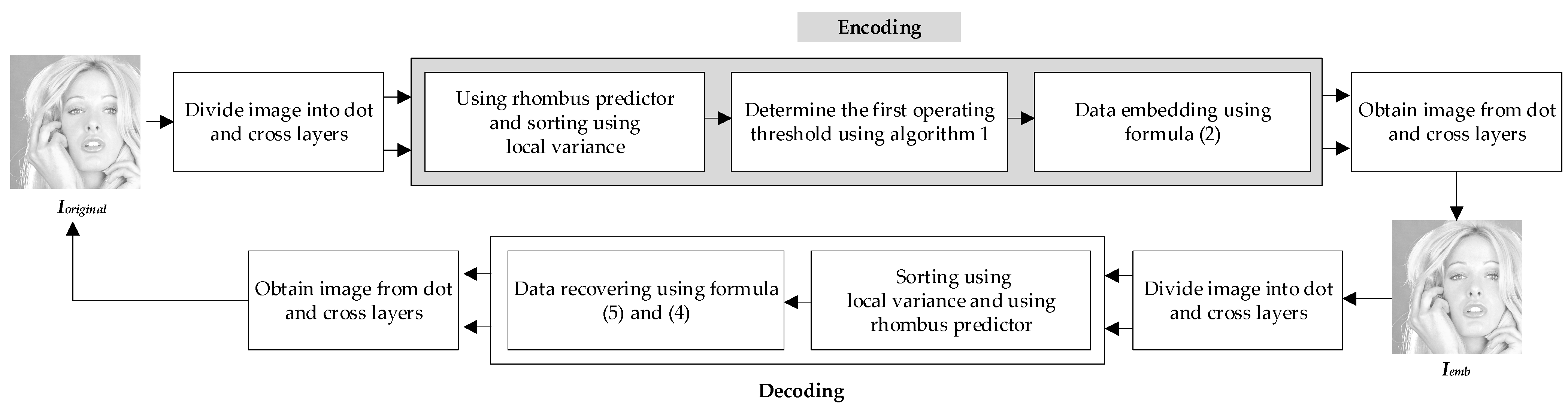
Our proposed method involves two layers, as described in [17], with half of the payload embedded in each layer. The encoding process for both layers is identical, so we will focus on describing the encoding of the first layer. It is important to note that our method includes a 28-bit footer, consisting of 8 bits for the operating threshold and 20 bits for the pixel order position of embedding. A simple block diagram of our encoding/decoding process is shown in Figure 7. The encoding algorithm can be summarized as follows:

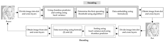
Figure 7. A simple block diagram for our encoding/decoding.

-

Step 1: For each pixel, calculate the predicted values, prediction errors, and local variance values according to [17].

-

Step 2: Sort the local variance values in ascending order to establish the pixel processing order. This order will be used for Steps 3 through 7.

-

Step 3: Set aside the last 28 pixels and gather their LSB (least significant bit) values.

-

Step 4: Determine the first operating threshold using the procedure outlined in algorithm 1.

-

Step 5: Use Equation (2) to embed the payload, the last 28 LSBs, and the location map. The location map is created with Equation (3), and this step is applied pixel by pixel.

-

Step 6: Create the footer, insert it into the last 28 LSBs, and then calculate the PSNR (Peak Signal-to-Noise Ratio).

-

Step 7: Increase the threshold t and return to Step 5. Stop the process when the PSNR starts decreasing.

For the decoding process, the layers are recovered in reverse order, starting from the last and moving to the first. The decoding algorithm is summarized as follows:

-

Step 1: Calculate the local variance values.

-

Step 2: Sort the local variance values in ascending order to establish the operating order for processing the pixels. This order is used for Steps 3 through 7.

-

Step 3: Extract the footer from the last 28 LSBs, which contains the operating threshold and the final embedding position.

-

Step 4: Compute the predicted values and prediction errors.

-

Step 5: Use Equation (5) to extract the payload, location map, and the original 28 LSBs.

-

Step 6: Recover the original pixel values using Equation (4).

-

Step 7: Restore the original 28 LSBs.

6. Experiments

6.1. Test Images

Nearly all previous RDH schemes have been tested on various natural grayscale images, including Lena, Baboon, Peppers, Sailboat, Fishing boat, Elaine, Airplane (F-16), Grass (D9), Car and APCs, Man, and Tiffany, which are available for download from [50], while Barbara can be obtained from [51]. The images are separated into two groups to illustrate the effectiveness of our proposed method by comparing with the famous algorithm [17] and two algorithms contained in [21,23], respectively:

(1)

Normally, the problematic pixels have intensities closer to the minimum or maximum. Hence, Man, Tiffany, Grass (D9), Sand, Car and APCs, Kodim06, Kodim10, and Kodim20 are considered to be elements of this group. To facilitate comparison, Man is resized into 512 × 512.

(2)

There are eight images in this group, Lena, Barbara, Baboon, Peppers, Fishing boat, Sailboat, Elaine, Airplane (F-16), Kodim12, Kodim14, Kodim16, and Kodim22. The intensities of these images are not close to the minimum or maximum. Thus, we can usually dispense with the location map from these images, unlike the first group.

The Kodak set includes 24 color images (24 bits). Each image is either 768 × 512 or 512 × 768 in size and they can be downloaded from [52]. For our experiments, we note that all color images were transformed into gray-scale versions by the rgb2gray command in MATLAB R2016a.

6.2. Experimental Results

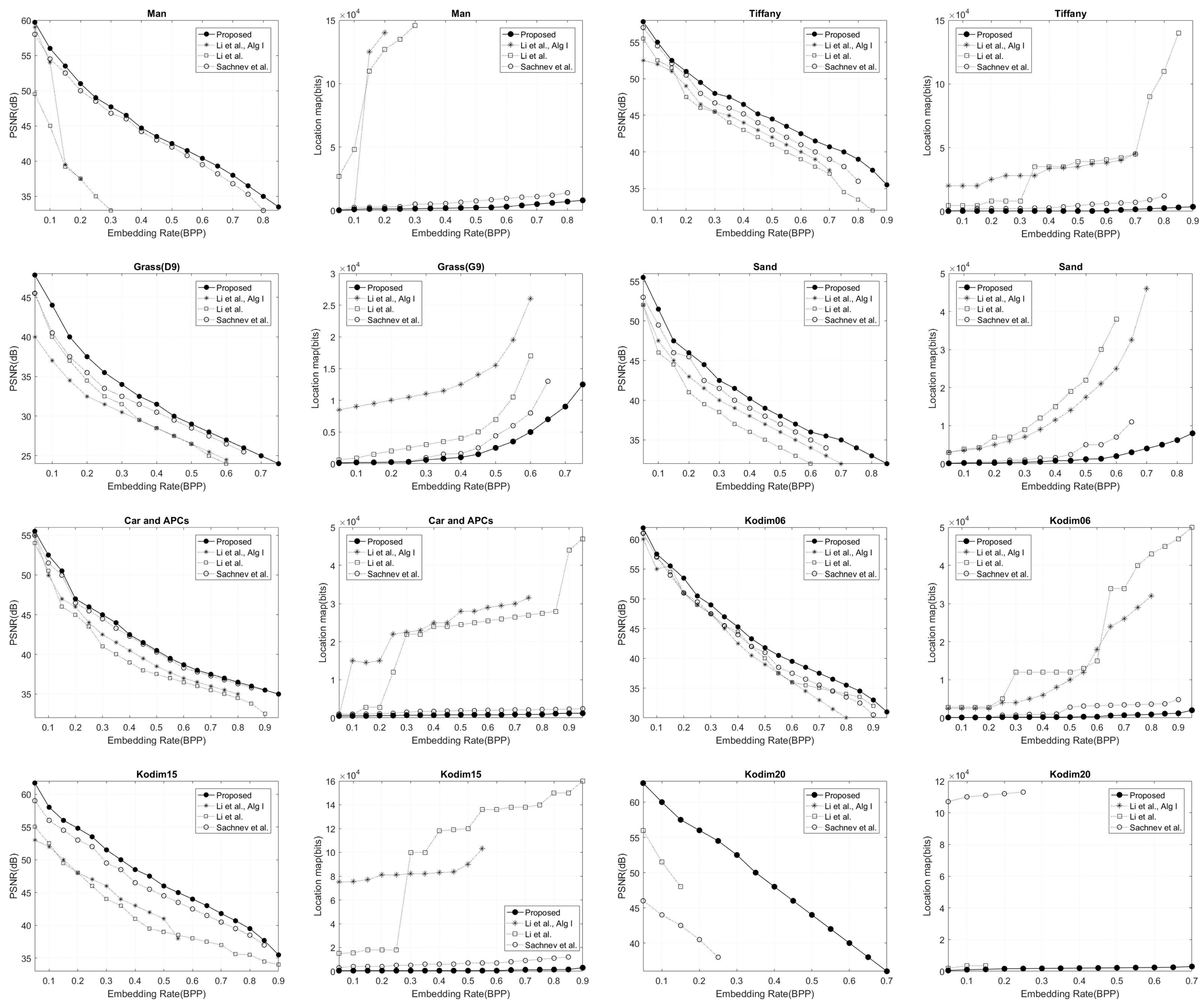
The experimental results obtained from the first group are plotted in Figure 8. For the results of Man, refs. [21,23] perform worse than [17] and our method. Notice that the result for Man is not presented in Figure 8 after the embedding rates equal 0.2 and 0.3 for [21,23] because these methods cannot embed such a payload into this image. The size of the location map is prohibitively high (around 15 × 10⁴ bits at 0.3 BPP for [21] and around 14 × 10⁴ bits at 0.2 BPP for [23]) because their location maps are recorded by correcting the position of overflow/underflow pixels which obviously impact the performance of these methods. The size of our location maps is reduced significantly as the embedding rate increases compared to the location maps of [17]. The size of the location maps at 0.3 BPP and 0.8 BPP are smaller by about 4.3 × 10³ bits and 9.5 × 10³ bits, respectively. There is an average improvement in gain compared with [17] of about 1.17 dB.

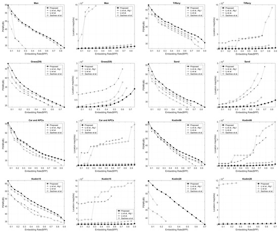
Figure 8. Embedding rate versus image distortion (end left and center right) and location map (center left and end right) for our approach in comparison with Sachnev et al. [17], Li et al. [21], and Li et al., algorithm I [23] on the first group and three Kodak images.

The latter result is obtained from Tiffany. Since the intensities of this image are close to maximum, it will greatly decrease the performance of [21,23], i.e., the surplus of [23] location map is about 2 × 10⁴ bits which is obtained by the pixels whose intensities have a maximum value. Our algorithm is also able to achieve higher image quality especially when payloads are high. For example, the gain in PSNR improves around 3 dB for [17] and almost 6.3 dB for [21] at 0.8 BPP. This great improvement is achieved by reducing the size of the location map. The average gain in PSNR of Tiffany is improved by about 1.34 dB, 2.85 dB and 3.65 dB compared with [17,21,23], respectively. The performance of any RDH scheme based on PEE and HS improves by minimizing the size of the location map. A smaller location map requires fewer embedding bits, which leads to smaller threshold values and, consequently, reduced distortion.

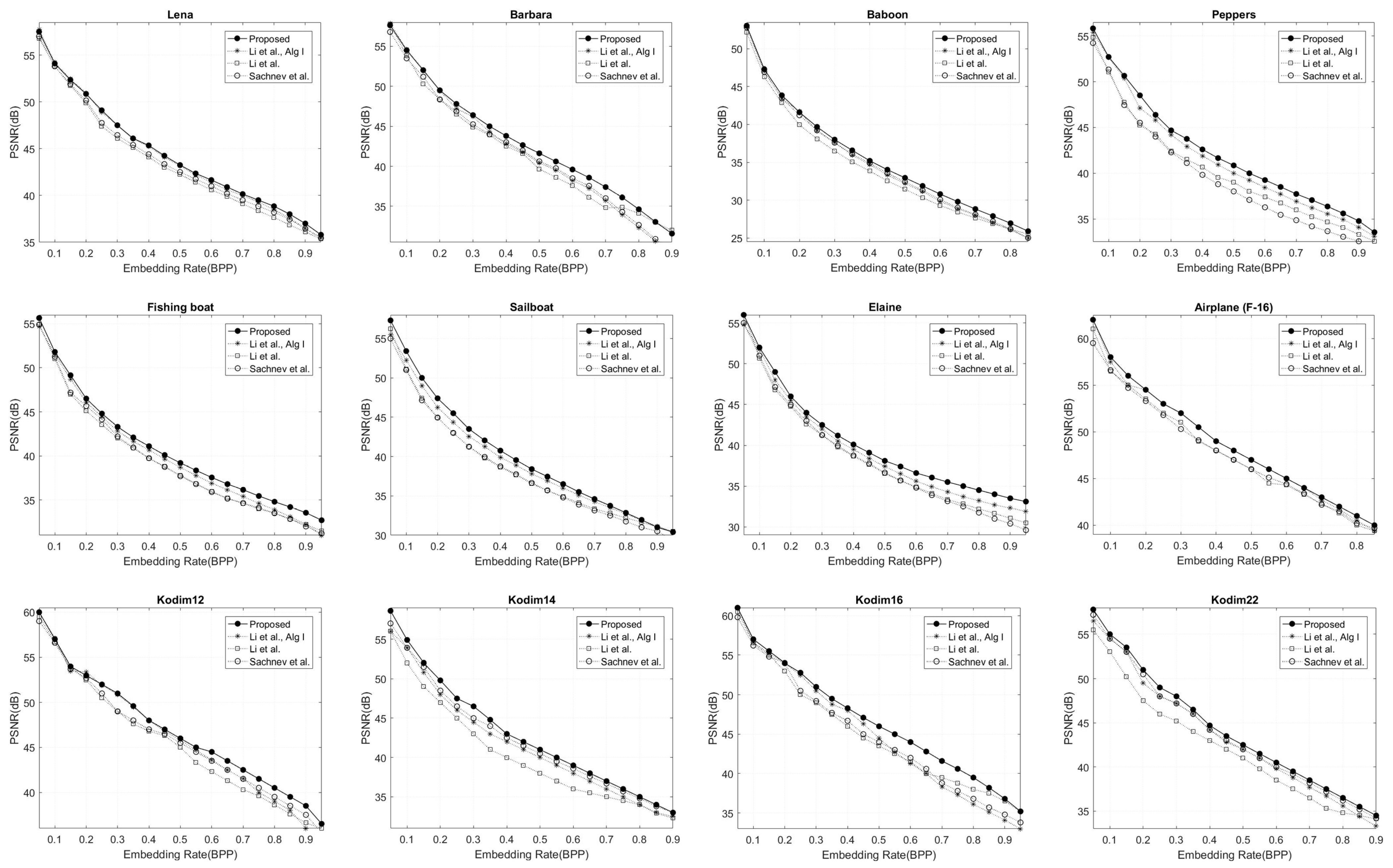
The results for the second group of images are shown in Figure 9. We can see that [17,21,23] are less efficient than our scheme for all images. The average gain in PSNR improves around 3.2, 2.6 and 1.3 dB for [17,21,23], respectively. Even in standard grayscale images where the intensity values do not approach the maximum and minimum values, our proposed method still results in low distortion due to the reduced size of the location maps. Table 2 compares the PSNR of the proposed method with the algorithms of Sachnev et al. [17], Li et al. [21], and Li et al. [23] at payloads of 0.2 and 0.8 BPP. The results indicate that the proposed method achieves superior PSNR values across various test images.

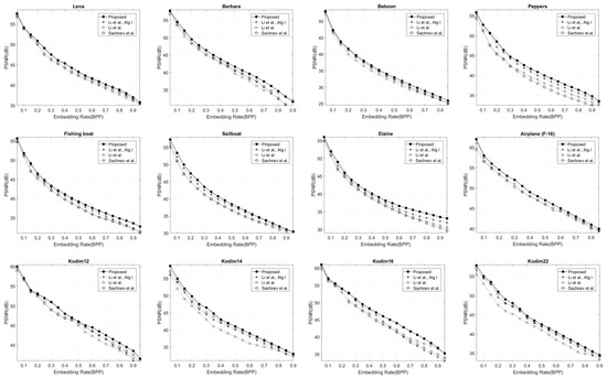
Figure 9. Embedding rate versus image distortion for our approach in comparison with Sachnev et al. [17], Li et al. [21], and Li et al. [23], algorithm I on the second group and four Kodak images.

Table 2. Comparison of PSNR between the proposed method and the algorithms of Sachnev et al. [17], Li et al. [21], and Li et al. [23] (algorithm I) for payloads of 0.2 and 0.8 BPP.

	PSNR (dB)
	0.2 BPP				0.8 BPP
Image	Ours	[17]	[21]	[23]	Ours	[17]	[21]	[23]
Lena	50.81	50.50	50.44	50.80	38.76	38.16	37.64	38.45
Barbara	49.71	48.52	49.17	49.43	35.03	33.73	31.17	32.07
Baboon	41.72	41.58	40.98	41.43	27.14	26.30	23.80	26.07
Peppers	48.90	45.63	49.11	47.02	36.87	33.73	36.81	35.49
Sailboat	47.75	45.23	47.85	46.21	33.32	31.66	32.72	32.78
Fishing boat	46.71	45.57	45.94	46.19	35.16	33.24	33.50	33.82
Elaine	45.94	44.52	45.61	45.34	34.01	31.01	33.58	32.69
Airplane(F-16)	54.34	53.20	53.95	54.29	41.18	40.94	39.25	40.42
Grass(D9)	37.58	35.47	32.03	32.74	-	-	-	-
Car and APCs	47.45	46.95	46.55	45.90	36.77	36.71	35.18	35.48
Sand	45.95	44.34	41.49	42.97	32.26	31.71	-	-
Tiffany	51.41	51.09	51.25	48.46	38.61	37.78	37.26	-
Man	50.98	50.66	48.97	36.83	34.88	35.37	30.89	-

7. Conclusions

In this paper, we proved that the infimums of SMT and DMT in terms of predicted value are $⌈-u^{\prime }/2⌉$ and $⌈-u^{\prime }/3⌉$, respectively, and the supremums of the SMT and DMT in terms of predicted value are $⌊(254-u^{\prime })/2⌋$ and $⌊(253-u^{\prime })/3⌋$, respectively. This implies that by limiting the non-positive and non-negative thresholds of each predicted value to their infimum and supremum, we maximize the number of embeddable pixels while minimizing the size of the location map. Using this result, we have presented the procedure to determine the first operating threshold. This greatly reduces the computational complexity of RDH. Additionally, we have created encoding and decoding formulas that do not rely on modification testing for RDH based on PEE and HS. The comparison with the famous [17,21,23] algorithms demonstrates that our algorithm outperforms or performs as well as these algorithms. An area of application of our method is in medical images where pixels have high variability as most pixels approach a minimum intensity value. In future research, adaptive predictors may be considered to provide flexible embedding.

References

- Fridrich, J.; Goljan, M.; Du, R. Lossless data embedding—New paradigm in digital watermarking. EURASIP J. Adv. Signal Process. 2002, 2002, 185–196. [Google Scholar] [CrossRef]
- Kalker, T.; Willems, F.M.J. Capacity bounds and constructions for reversible data hiding. In Proceedings of the 2002 14th International Conference on Digital Signal Processing Proceedings, Santorini, Greece, 1–3 July 2002. [Google Scholar]
- Celik, M.U.; Sharma, G.; Tekalp, A.M.; Saber, E. Lossless generalized-LSB data embedding. IEEE Trans. Image Process. 2005, 14, 253–266. [Google Scholar] [CrossRef] [PubMed]
- Celik, M.U.; Sharma, G.; Tekalp, A.M. Lossless watermarking for image authentication: A new framework and an implementation. IEEE Trans. Image Process. 2006, 15, 1042–1049. [Google Scholar] [CrossRef]
- Tian, J. Reversible data embedding using a difference expansion. IEEE Trans. Circuits Syst. Video Technol. 2003, 13, 890–896. [Google Scholar] [CrossRef]
- Alattar, A.M. Reversible watermark using the difference expansion of a generalized integer transform. IEEE Trans. Image Process. 2004, 13, 1147–1156. [Google Scholar] [CrossRef]
- Kamstra, L.; Heijmans, H.J.A.M. Reversible data embedding into image using wavelet techniques and sorting. IEEE Trans. Image Process. 2005, 14, 2082–2090. [Google Scholar] [CrossRef]
- Kim, H.J.; Sachnev, V.; Shi, Y.Q.; Nam, J.; Choo, H.G. A novel difference expansion transform for reversible data embedding. IEEE Trans. Inf. Forensics Secur. 2008, 4, 456–465. [Google Scholar]
- Lee, S.; Yoo, C.D.; Kalker, T. Reversible image watermarking based on integer-to-integer wavelet transform. IEEE Trans. Inf. Forensics Secur. 2007, 2, 321–330. [Google Scholar] [CrossRef]
- Coltuc, D. Low distortion transform for reversible watermarking. IEEE Trans. Image Process. 2012, 21, 412–417. [Google Scholar] [CrossRef]
- Wang, X.; Shao, C.; Xu, X.; Niu, X. Reversible Data-Hiding Scheme for 2-D Vector Maps Based on Difference Expansion. IEEE Trans. Inf. Forensics Secur. 2007, 2, 311–320. [Google Scholar] [CrossRef]
- Ni, Z.; Shi, Y.Q.; Ansari, N.; Su, W. Reversible data hiding. IEEE Trans. Circuits Syst. Video Technol. 2006, 16, 354–362. [Google Scholar]
- Thodi, D.M.; Rodriguez, J.J. Prediction-error-based reversible watermarking. In Proceedings of the 2004 IEEE International Conference on Image Processing, Singapore, 24–27 October 2004. [Google Scholar]
- Thodi, D.M.; Rodriguez, J.J. Reversible watermarking by prediction-error expansion. In Proceedings of the 2004 IEEE Southwest Symposium on Image Analysis and Interpretation, Lake Tahoe, NV, USA, 28–30 March 2004. [Google Scholar]
- Thodi, D.M.; Rodriguez, J.J. Expansion embedding techniques for reversible watermarking. IEEE Trans. Image Process. 2007, 16, 721–730. [Google Scholar] [CrossRef] [PubMed]
- Hu, Y.; Lee, H.K.; Li, J. DE-based Reversible data hiding with improved overflow location map. IEEE Trans. Circuits Syst. Video Technol. 2009, 19, 250–260. [Google Scholar]
- Sachnev, V.; Kim, H.J.; Nam, J.; Suresh, S.; Shi, Y.Q. Reversible watermarking algorithm using sorting and prediction. IEEE Trans. Circuits Syst. Video Technol. 2009, 19, 989–999. [Google Scholar] [CrossRef]
- Lou, L.; Chen, Z.; Chen, M.; Zeng, X.; Xiong, Z. Reversible image watermarking using interpolation technique. IEEE Trans. Inf. Forensics Secur. 2010, 5, 187–193. [Google Scholar]
- Hwang, H.J.; Kim, H.J.; Sachnev, V.; Joo, S.H. Reversible watermarking method using optimal histogram pair shifting based on prediction and sorting. KSII Trans. Internet Inf. Syst. 2010, 4, 655–670. [Google Scholar] [CrossRef]
- Coltuc, D. Improved embedding for prediction-based reversible watermarking. IEEE Trans. Inf. Forensics Secur. 2011, 6, 873–882. [Google Scholar] [CrossRef]
- Li, X.; Yang, B.; Zeng, T. Efficient reversible watermarking based on adaptive prediction-error expansion and pixel selection. IEEE Trans. Image Process. 2011, 20, 3524–3533. [Google Scholar]
- Dragoi, C.; Coltuc, D. Improved rhombus interpolation for reversible watermarking by difference expansion. In Proceedings of the 20th European Signal Processing Conference (EUSIPCO), Bucharest, Romania, 27–31 August 2012. [Google Scholar]
- Li, X.; Li, B.; Yang, B.; Zeng, T. General Framework to Histogram-Shifting-Based Reversible Data Hiding. IEEE Trans. Image Process. 2013, 22, 2181–2191. [Google Scholar] [CrossRef]
- Ou, B.; Li, X.; Zhao, Y.; Ni, R. Reversible data hiding based on PDE predictor. J. Syst. Softw. 2013, 86, 2700–2709. [Google Scholar] [CrossRef]
- Coatrieux, G.; Pan, W.; Cuppens-Boulahia, N.; Cuppens, F.; Roux, C. Reversible watermarking based on invariant image classication and dynamic histogram shifting. IEEE Trans. Inf. Forensics Secur. 2013, 8, 111–120. [Google Scholar] [CrossRef]
- Panyindee, C.; Pintavirooj, C. Optimal gaussian weight predictor and sorting using genetic algorithm for reversible watermarking based on PEE and HS. IEICE Tran. Inf. Syst. 2016, E99, 2306–2319. [Google Scholar] [CrossRef]
- Yin, Z.; Chen, L.; Lyu, W.; Luo, B. Reversible attack based on adversarial perturbation and reversible data hiding in YUV colorspace. Pattern Recognit. Lett. 2023, 166, 1–7. [Google Scholar] [CrossRef]
- Qin, C.; Zhang, W.; Cao, F.; Zhang, X.; Chang, C.-C. Separable reversible data hiding in encrypted images via adaptive embedding strategy with block selection. Signal Process. 2018, 153, 109–122. [Google Scholar] [CrossRef]
- Qin, C.; Jiang, C.; Mo, Q.; Yao, H.; Chang, C.-C. Reversible data hiding in encrypted image via secret sharing based on GF(p) and GF(28). IEEE Trans. Circuits Syst. Video Technol. 2022, 32, 1928–1941. [Google Scholar]
- Li, Q.; Ma, B.; Wang, X.; Wang, C.; Gao, S. Image steganography in color conversion. IEEE Trans. Circuits Syst. 2024, 71, 106–110. [Google Scholar] [CrossRef]
- Li, Q.; Ma, B.; Fu, X.; Wang, X.; Wang, C.; Li, X. Robust image steganography via color conversion. IEEE Trans. Circuits Syst. Video Technol. 2024, 35, 1399–1408. [Google Scholar] [CrossRef]
- He, J.; Chen, J.; Tang, S. Reversible data hiding in JPEG images based on negative influence models. IEEE Trans. Inf. Forensics Secur. 2020, 15, 2121–2133. [Google Scholar] [CrossRef]
- Yin, Z.; Ji, Y.; Luo, B. Reversible data hiding in JPEG images with multi-objective optimization. IEEE Trans. Circuits Syst. Video Technol. 2020, 30, 2343–2352. [Google Scholar]
- Xiao, M.; Li, X.; Ma, B.; Zhang, X.; Zhao, Y. Efficient reversible data hiding for JPEG images with multiple histograms modification. IEEE Trans. Circuits Syst. Video Technol. 2021, 31, 2535–2546. [Google Scholar] [CrossRef]
- Qiu, Y.; Qian, Z.; He, H.; Tian, H.; Zhang, X. Optimized lossless data hiding in JPEG bitstream and relay transfer-based extension. IEEE Trans. Circuits Syst. Video Technol. 2021, 31, 1380–1394. [Google Scholar] [CrossRef]
- Du, Y.; Yin, Z.; Zhang, X. High capacity lossless data hiding in JPEG bitstream based on general VLC mapping. IEEE Trans. Dependable Secur. Comput. 2022, 19, 1420–1433. [Google Scholar] [CrossRef]
- Weng, S.; Zhang, T. Adaptive reversible data hiding for JPEG images with multiple two-dimensional histograms. J. Vis. Commun. Image Represent. 2022, 85, 103487. [Google Scholar] [CrossRef]
- Yu, C.; Cheng, S.; Zhang, X.; Zhang, X.; Tang, Z. Reversible Data Hiding in Shared JPEG Images. ACM Trans. Multimed. Comput. Commun. Appl. 2024, 20, 1–24. [Google Scholar] [CrossRef]
- Yang, X.; Wang, Y.; Huang, F. CNN-Based Reversible Data Hiding for JPEG Images. IEEE Trans. Circuits Syst. Video Technol. 2024, 34, 11798–11809. [Google Scholar] [CrossRef]
- Lyu, W.-L.; Cheng, L.; Yin, Z. High-capacity reversible data hiding in encrypted 3D mesh models based on multi-MSB prediction. Signal Process. 2022, 201, 108686. [Google Scholar] [CrossRef]
- Peng, F.; Liao, T.; Long, M. A semi-fragile reversible watermarking for authenticating 3D models in dual domains based on variable direction double modulation. IEEE Trans. Circuits Syst. Video Technol. 2022, 32, 8394–8408. [Google Scholar] [CrossRef]
- Qu, L.; Lu, H.; Chen, P.; Amirpour, H.; Timmerer, C. Ring Co-XOR encryption based reversible data hiding for 3D mesh model. Signal Process. 2024, 217, 109357. [Google Scholar] [CrossRef]
- Wu, H.-T.; Cao, X.; Jia, R.; Cheung, Y.-M. Reversible data hiding with brightness preserving contrast enhancement by two-dimensional histogram modification. IEEE Trans. Circuits Syst. Video Technol. 2022, 32, 7605–7617. [Google Scholar] [CrossRef]
- Zhang, T.-C.; Hou, T.-S.; Weng, S.-W.; Zou, F.-M.; Zhang, H.-C.; Chang, C.-C. Adaptive reversible data hiding with contrast enhancement based on multi-histogram modification. IEEE Trans. Circuits Syst. Video Technol. 2022, 32, 5041–5054. [Google Scholar] [CrossRef]
- Qi, W.; Guo, S.; Hu, W. Generic reversible visible watermarking via regularized graph fourier transform coding. IEEE Trans. Image Process. 2022, 31, 691–705. [Google Scholar] [CrossRef] [PubMed]
- Tang, X.; Wang, H.; Chen, Y. Reversible data hiding based on a modified difference expansion for H.264/AVC video streams. Multimed. Tools Appl. 2020, 79, 28661–28674. [Google Scholar] [CrossRef]
- Xu, D.; Liu, Y. Reversible data hiding in H.264/AVC videos based on hybrid-dimensional histogram modification. Multimed. Tools Appl. 2022, 81, 29305–29319. [Google Scholar] [CrossRef]
- Yang, Y.; Zou, T.; Huang, G.; Zhang, W. A high visual quality color image reversible data hiding scheme based on B-R-G embedding principle and CIEDE2000 assessment metric. IEEE Trans. Circuits Syst. Video Technol. 2022, 32, 1860–1874. [Google Scholar] [CrossRef]
- Zhang, C.; Ou, B.; Li, X.; Xiong, J. Human visual system guided reversible data hiding based on multiple histograms modification. Comput. J. 2023, 66, 888–906. [Google Scholar] [CrossRef]
- The USC-SIPI Image Database, Miscellaneous. Available online: http://sipi.usc.edu/database/database.php?volume=misc (accessed on 11 October 2024).
- Miscelaneous Gray Level Images (512 × 512). Available online: http://decsai.ugr.es/cvg/dbimagenes/g512.php (accessed on 11 October 2024).
- Kodak Lossless True Color Image Suite. Available online: http://r0k.us/graphics/kodak/ (accessed on 18 March 2024).
Disclaimer/Publisher’s Note: The statements, opinions and data contained in all publications are solely those of the individual author(s) and contributor(s) and not of MDPI and/or the editor(s). MDPI and/or the editor(s) disclaim responsibility for any injury to people or property resulting from any ideas, methods, instructions or products referred to in the content. |
© 2025 by the author. Licensee MDPI, Basel, Switzerland. This article is an open access article distributed under the terms and conditions of the Creative Commons Attribution (CC BY) license (https://creativecommons.org/licenses/by/4.0/).