Enhancing Driving Control via Speech Recognition Utilizing Influential Parameters in Deep Learning Techniques

Abstract

This study investigates the enhancement of automated driving and command control through speech recognition using a Deep Neural Network (DNN). The method depends on some sequential stages such as noise removal, feature extraction from the audio file, and their classification using a neural network. In the proposed approach, the variables that affect the results in the hidden layers were extracted and stored in a vector to classify them and issue the most influential ones for feedback to the hidden layers in the neural network to increase the accuracy of the result. The result was 93% in terms of accuracy and with a very good response time of 0.75 s, with PSNR 78 dB. The proposed method is considered promising and is highly satisfactory to users. The results encouraged the use of more commands, more data processing, more future exploration, and the addition of sensors to increase the efficiency of the system and obtain more efficient and safe driving, which is the main goal of this research.

1. Introduction

With the rapid development of intelligent transportation systems, it has become important to enhance vehicle control to ensure their safety and use modern technologies in these systems. Speech recognition to provide driving comfort represents a promising path, especially when enhanced by one of the Artificial Intelligence (AI) methods by Bengio, Y. et al., including deep learning technology [1], because of the automatic reaction speed and not getting bored with time. To provide safer and more efficient driving, many applications illustrated by Ofer, D. et al. focus on natural language understanding, and language is the ideal way to interact with people, but for a long time, the interaction between machines and humans has lacked language interpretation [2]. With the development shown by Rastgoo R. et al., language recognition has become the focus of interest for students and researchers to open horizons for dealing with machines [3]. Current systems in mobile devices, such as Apple Siri and Google Now, recognize speeches but are considered simplistic and unreliable because they do not simulate the risks that arise from differentiating conversations [4]. The risks lie in the accuracy of the command and the severity of the differentiation in response, which may lead to human risks.

A study by McCallum, M.C., et al. Integrating speech recognition technology into driving control systems can help significantly reduce driver distraction [5]. This allows for reduced hand-holding and increased AI in cars. Traditional speech recognition systems need more effort in the driving environment and thus are difficult to handle with noise, multiple accents, and different speech patterns [6]. Deep learning offers a promising and viable solution to these challenges in dealing with big data. This study utilizes the proposed deep learning model and integrates high-impact variables (derived from the features extracted from the voice that control the system) through a repetitive processing process, which is a key feature in speech recognition and is based on the frequencies suggested by Dhanjal, A.S. and Singh, W. that accompany all hidden layers in the neural network [7]. These variables can be described as tonal features (associated with certain voice signals), environmental factors, noise, or acoustic differences.

The claim that deep learning significantly enhances speech recognition capabilities requires further substantiation, as presented by Kumar, Y., due to existing gaps and challenges [8]. While deep learning has demonstrated substantial improvements, particularly in Word Error Rates (WER) and handling diverse data, its reliance on large, diverse datasets makes it less effective for under-represented languages or accents [9]. Additionally, its computational demands limit deployment in resource-constrained environments. Benchmarks often favor deep learning models but may not fully represent real-world complexities. Furthermore, bias, generalizability, and ethical concerns highlight the need for comprehensive validation. To solidify the claim, broader empirical evidence and nuanced analyses are essential.

The main goal here is to develop a precise speech control system for driving that provides immediate, real-time response. This, in turn, provides comfort and safety for drivers, and by leveraging the power of deep learning to harness high-impact variables that adapt during processing, our system is in line with the efforts leading to the integration of AI into everyday life. Then, speech recognition plays a key role in reducing distortion during driving. The study aims to achieve the following objectives:

• To develop a new automated driving system: Create an innovative automated driving system by leveraging sophisticated deep learning methodologies.
• To improve DNN with influential parameters: Improve the efficiency of deep neural networks by integrating influential variables that are pertinent to driving control, examine the effects of modifying the hidden layers in the network, and incorporate feedback acknowledgments to achieve optimal adjustment.

Contributions of this study are illustrated by improving speech recognition by controlling the neural network layers with influential parameters. Update the deep neural network according to the best weight of the features extracted from the speech, which depends on the loss function and gradient descent, to obtain the highest iterations in the training process for the best prediction.

2. Related Work

In the field of speech recognition, few studies were conducted, which were included in reviews from 2006 to 2018 [10]. It mentioned the techniques used, which relied on the deep neural network, and more than 174 studies that used artificial intelligence methods, statistical techniques, and mathematical analysis. The thesis gives the importance of using deep learning in the study. Different techniques were used, such as Deep Belief Network (DBN) [11] and Convolutional Neural Network (CNN) [12], and most studies relied on deep learning [13]; this makes work easier and improved in a study that provided an overview of deep learning in language recognition and speech recognition [14]. Many studies have been presented that are interested in the Recurrent Neural Network (RNN) model and how to improve performance and training data [15], which reflects the importance of training at work, as well as CNN algorithms [16], that help in improvements to these algorithms, and the integration of a lot of complex linguistic knowledge. In many studies, the audio model, which is considered the internal line of the artificial intelligence system [17], was enhanced, and the literal meaning of speech was extracted, which is the basis for the results of studies with control over machines. One of the most important studies that addressed a noisy environment for extracting speech through deep learning considered natural language, which took advantage of the maximum benefit from deep education and its advantages [18], which opened horizons towards intensifying efforts to prevent noise from hiding the literal text of speech. Speech recognition with developed models and working on many dialects are important for this study. A study was conducted by reviewing the oral interface devices that work on sensors to recognize speech using the deep learning algorithm [19]. Another study also reviewed the research that is interested in recognizing Arabic speech and the deep learning algorithm [20] that gives priority to the use of deep education techniques in processing audio files. A special study was presented on the multiplicity of dialects and how to distinguish them through deep learning [21], which is considered the appropriate environment for these problems. Another review focused on speech recognition in smart devices using deep learning and confirmed an accuracy rate of 90% [22], and then another method relied on hidden Markov models (HMMs) [23], which addressed related problems that improved the result of artificial intelligence by increasing training and concluded that training leads to accuracy in the result but a delay in time. Speech recognition traces back several decades, starting with HMM algorithms, followed by the big breakthrough of SRS using neural networks with natural language processing. A decade later, deep neural networks were used in Speech Recognition System (SRS) systems [24], which recommended the use of this technique for better accuracy. As neural networks generally replaced the traditional Gaussian mixture, the hybrid approach also took its influence from these methods to find the best solutions. With the development of artificial intelligence algorithms, deep learning has become the best way to solve the problem of speech discrimination.

Speech recognition in its early attempts at voice control was done by traditional machine learning algorithms, including HMMs and Gaussian mixture models (GMMs), which show the importance of removing noise from the audio file. These were effective and accurate in controlled environments but suffered from several issues, including variance and noise in the real world, and many studies have addressed the advantages and disadvantages of these models.

In terms of deep learning, its emergence has significantly enhanced speech recognition capabilities. Research in [25] confirmed the superiority of deep neural networks in this field over traditional methods, giving the reason for using deep learning in speech recognition. The study in [26] confirmed the accuracy of the comprehensive deep learning model by distinguishing languages in high-noise environments, and these studies laid the main foundation for the application of deep learning in various fields and specializations that require vocal controls. Recent research has focused on improving speech recognition systems, especially in driving, due to the technological and industrial development in this field. [27] Proposed a new approach that combines convolutional neural networks (CNNs) and recurrent neural networks (RNNs) to recognize speech in a noisy environment due to the work environment and noise removal. Another study, [28], relied on deep learning in the challenges of natural languages in control systems in general; it gave importance to the use of deep education in our field of study.

Speech Recognition (Deep Learning and Deep Neural Networks)

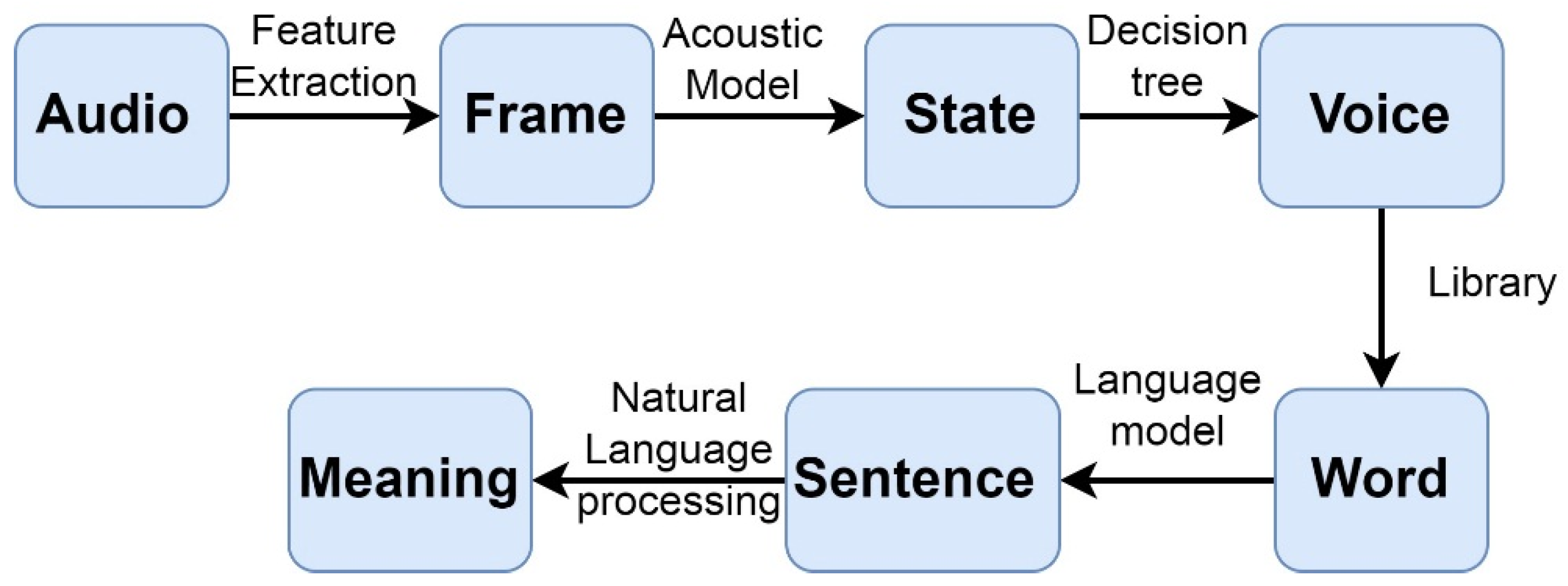
One of the famous technologies is speech recognition technology, which enables the machine to understand language and commands. It is one of the leading technologies in the field of computers and control in general, so we can formulate commands in a way that the computer understands. Thus, we can benefit from it in automating control devices [23]. Natural language processing is a concept that refers to the combination of languages and machine learning. Using multiple models to teach machines to understand natural languages is considered an application of machine learning. A sub-field of it is speech recognition, which means that computers understand what we say in languages. This is the specialty of computer science, as shown in Figure 1.

Figure 1. Speech Recognition Process (https://medium.com).

In terms of technological development, speech recognition has a long history in many technological applications. Recently, it has developed a lot when deep learning was used, as well as when using big data, and it has been significantly improved not only in terms of academic papers and research published in this regard but also in its use in the global industry and information technology, such as in global companies such as Google, Facebook, and Microsoft [29].

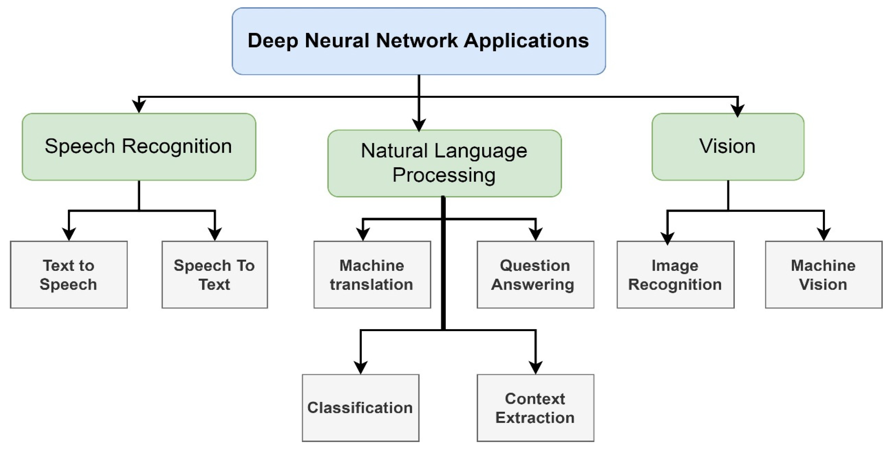
Currently, there are many techniques (such as machine learning and statistical learning) that work to increase the accuracy of speech recognition systems, including adding noise to the background, increasing the processed data, or changing the pitch. There are also hybrid methods that combine more than one method into one algorithm to improve speech recognition performance. The nature of language and the multiplicity of dialects for each of them leads to the need to increase accuracy and improve systems in linguistic contexts [30]. One of the reasons for not fully achieving the goals is natural language processing and the processing and interpretation that it entails, which leads to some difficulties in this field. Therefore, scientists have been keen to change the policy and method of processing that deals with the nature of language [31], as shown in Figure 2.

Figure 2. Natural Language Processing [32].

Deep learning refers to an artificial neural network architecture consisting of several layers [33]. Each layer represents a basic processing for a specific purpose. The concept of deep learning has been somewhat old since 1958 [34], and with the development of information technology and computers in terms of speed, storage, and big data, the concept of deep neural networks began to perform better than classical machine learning methods. In this section, we will discuss what is related to deep learning and its relation to speech recognition. Artificial intelligence technologies are used in many applications, including controlling electrical power [35,36], maintaining data security [37,38], and distinguishing human and robotic movement [39,40].

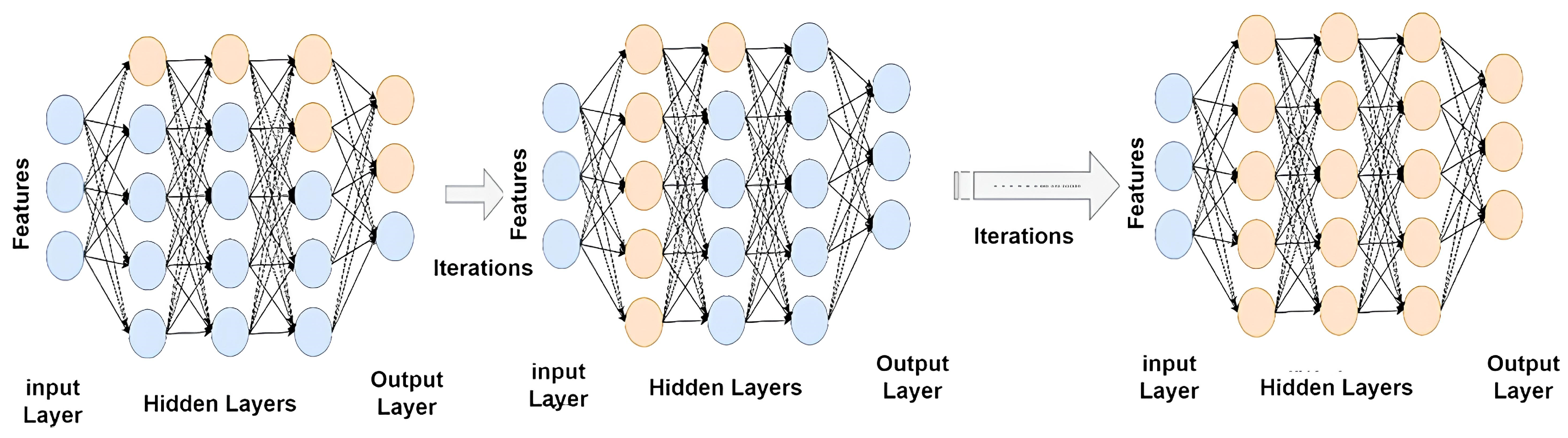
Deep learning is different from machine learning and artificial intelligence in general in that it requires very little human intervention. Deep learning came to address problems that machine learning could not address, and the result was unsatisfactory [17]. Through deep learning and its multiple hidden layers, a significant improvement can be achieved. Since the beginning of deep learning, developments have accompanied it through inferring hidden layers and back-propagation technology, as the training process has become easier than before [41]. The deep neural network is one of the deep learning methods, and its mention is linked to big data and data science in general. Many scientific and engineering problems have been addressed by predicting data outputs in advance, and there are many applications that the deep neural network has addressed, including speech recognition, as shown in Figure 3.

Figure 3. DNN Applications [17].

Deep learning is a simulation model of the human brain and a technically advanced approach to machine learning. When training on large data after several iterations, the algorithm makes decisions without human assistance automatically. Some data must be provided to the deep learning model, such as inputs, the desired result, and preprocessing, such as removing some noise. Data preprocessing is very important in the training process, as the performance measure here is important and necessary. In artificial neural networks (ANN), features and their extraction are important as an independent part that helps in the prediction process [42]. The work of the artificial neural network is almost similar to that of biological neurons, where weights and inputs play a fundamental role in finding the outputs. The layers of the neural network are closely connected to each other, as well as the nodes that make up those layers, and sometimes, the nodes of a certain layer are connected to the nodes of the previous or next layer. The error function is calculated from those weights and network connections. The result that comes out of the output layer is compared with the previously defined result if it is not suitable, and it is reprocessed with a new iteration. By iterating the rest of the data in the training mode, the model is taught, and the weights are saved for that training to perform the testing mode.

Unsupervised learning is the most important type of deep learning, in which the data is labeled before training, and the result is similar to the actual result [43]. This is one of the most important types of deep learning, as shown in Figure 4.

Figure 4. Unsupervised deep learning.

3. Method

The proposed methodology includes developing a speech recognition system for driving a car by using a deep learning algorithm and improving the deep neural network by exploiting the highly influential variables of the features extracted from the sound waveform. It consists of several main stages that complement each other and are equally important. There are main stages interspersed with sub-stages, such as data acquisition and collection from the main dataset and then extracting the features that are considered the cornerstone on which the contribution here is built. After that, the preprocessing begins to be prepared to build and develop an appropriate neural network system according to the strong influences in the system. When there is no satisfactory result, the structure of the deep neural network is changed to suit the external parameters and extracted features, and the process is repeated until we reach a satisfactory result. The flowchart in Figure 5 shows the main steps in the proposed system.

Figure 5. General flowchart of the proposed method.

3.1. Data Acquisition

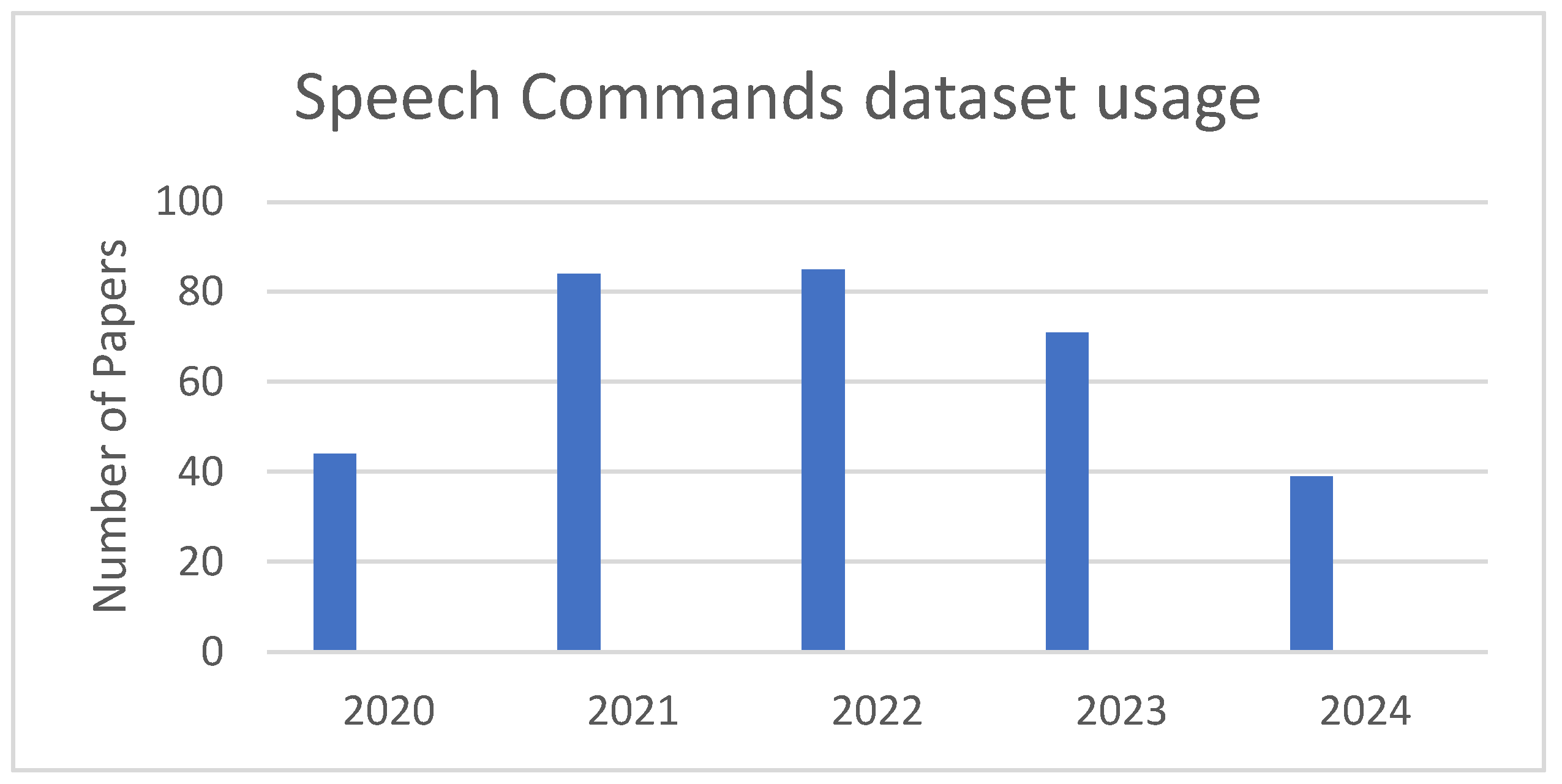
The standard dataset contains a large set of speech commands in audio format, including some of the commands used in this research. The speech command dataset is designed to help in the training process and the recognition of different speech commands. It contains single words, which is what we are interested in here, and sentences of several words, some of which contain strong noise, others less, and a smaller portion does not contain noise. The audio files are known and tagged for ease of training. They are usually 1–3 s audio files in a background noise. The dataset downloaded from https://arxiv.org/abs/1804.03209, accessed on 22 August 2024 is called speech commands and is 3.8 GB in size [44]. Many current studies have used this dataset, and its worth has been proven, as shown in Figure 6.

Figure 6. Availability of dataset.

3.2. Preprocessing (Noise Reduction)

Background noise is an important consideration because driving is accompanied by noise such as external sound, engine noise, or passenger conversations. Therefore, artificial noise is added to train the system to separate it and simulate real driving conditions. First, we have a speech file that contains noise, and the goal is to make it clean and noise-free so that it can be recognized well as:

$$y\left[n\right]=s\left[n\right]+d\left[n\right].$$

For example, y[n] is considered to be sampled noisy speech, s[n] is considered clean speech, and d[n] is considered additive noise and assumed = 0. This is not related to speech because speech signals are considered non-stationary with time variants. The noisy speech is processed frame by frame. The representation in the short-time Fourier transform (STFT) is given by:

$$Y\left(w,k\right)=S\left(w,k\right)+D(w,k)$$

Then, k is considered as the frame number, so we take the frames as single, and then k is neglected. And because of uncorrelated speech with background noise, the y[n] will be no cross term, such as:

$${\left|Y\left(w\right)\right|}^2={\left|S\left(w\right)\right|}^2+{\left|D\left(w\right)\right|}^2$$

Then, can subtract noise from speech or receiving files like:

$${\left|\widehat{S}\left(w\right)\right|}^2={\left|Y\left(w\right)\right|}^2-{\left|\widehat{D}\left(w\right)\right|}^2$$

${\left|\widehat{D}\left(w\right)\right|}^2$ is noise spectrum where can estimate the average speech frames as:

$${\left|\widehat{D}\left(w\right)\right|}^2={\displaystyle \frac{1}{M}}{\sum }_{j=0}^{M-1}{\left|Y_{SPj}\left(w\right)\right|}^2$$

Consider M as the number of frames of speech pauses (SP). Illustrated in Figure 7.

Figure 7. (a) Clean speech file and (b) noisy speech.

The noise can be reduced by responding to a high pass filter, where the frequency response is illustrated in Figure 8. While the blue curve considers the gain (amplitude) for the filter within different frequencies, one can notice that the frequency below the cutoff of 200 Hz (red dashed line) will be attenuated, which represents the reduction in it. The frequency above is okay and passed at least with less attenuation. The 3 dB cutoff level, which is the green dashed line around 0.7, is considered as the point refer gain under 70% from the maximum value, and it is used to define the cutoff. We can illustrate this mathematically as:

$$H\left(f\right)={\displaystyle \frac{1}{1+{\frac{f_c}{f}}^2}}$$

which represents a simple first order in HPF in this transfer function. f represents the frequency of the input signal, and $f_c$ is considered as cutoff frequency, and the pass frequency is higher than $f_c$ which reduces the frequency under $f_c$ which represents the noise.

Figure 8. Noise Reduction within HPF.

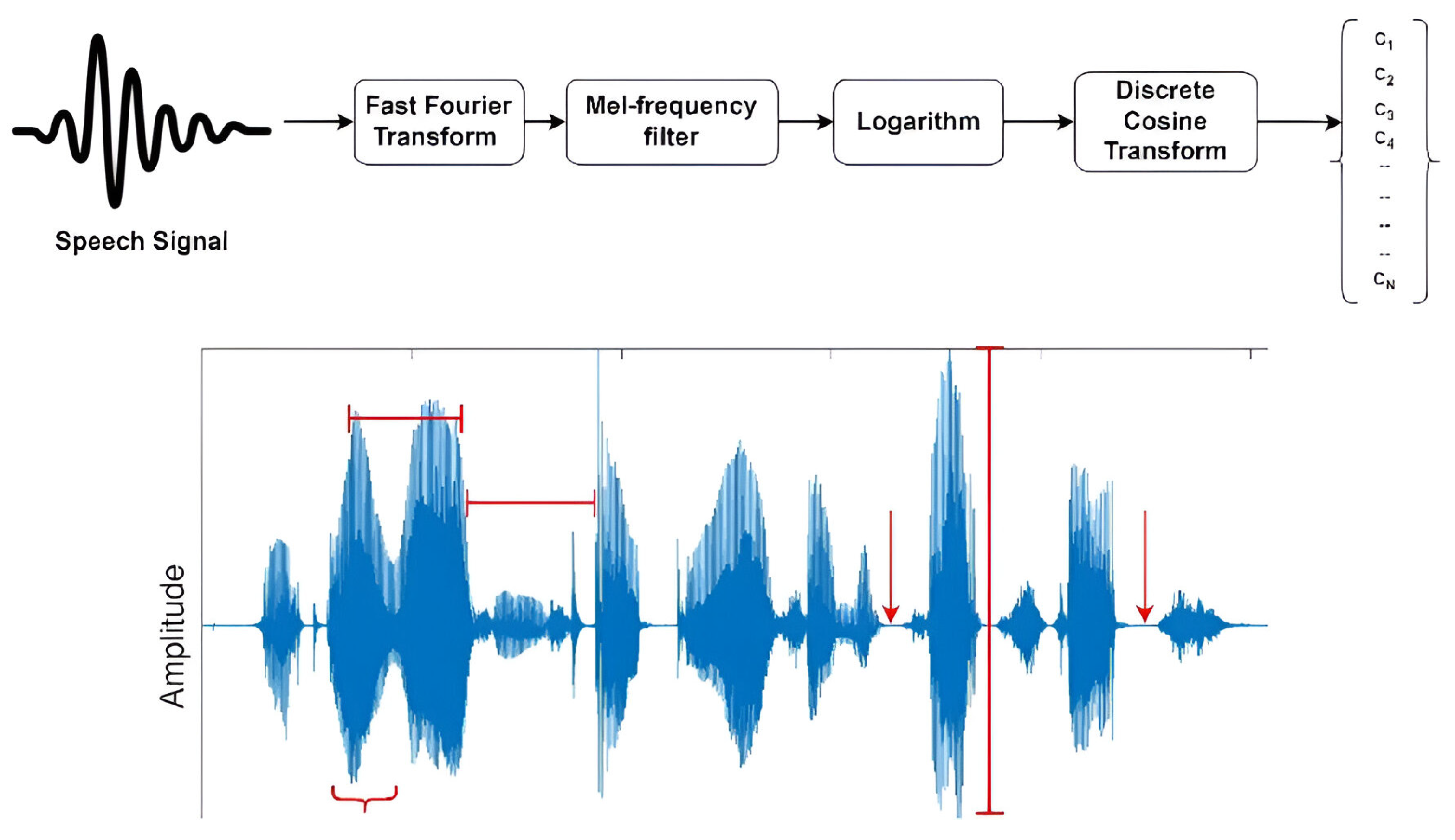
3.3. Feature Extraction

Speech is a human skill, and features are extracted by converting it into waveforms for subsequent processing. The extracted features include discrete waveform transforms, MFCCs, linear spectral frequencies, linear prediction coefficients (LPCs), perceptual linear prediction, etc. In speech enhancement, it refers to the enhancement of higher frequencies, then the signal is divided into short frames and then multiplied by a window function to separate the frequencies, after which filters are applied to obtain the frequency range and wavelength of each speech file, as shown in Figure 9.

Figure 9. Feature Extraction Process.

The extracted features are stored in a single vector containing the feature types. If there is more than one feature for each type, they are stored in other vectors and used in processing and classification in the following rounds after passing the first round.

3.4. Classification

The contribution lies in extracting the highly influential weights in the feedback to the previous stages of any of the layers of the neural network, which works to change the outcome of the layers in the neural network. All feedback through the layers affects the result in a certain way and to varying degrees, so those weights are stored in a special vector in order to classify those weights and extract the weights that have an effective effect on the result. This process is done several times (within iteration) until a result with the highest accuracy that matches the label in the training mode is obtained, as shown in Figure 10.

Figure 10. Structure of neural network with the proposed method through weighted extraction.

The process of restructuring the neural networks based on highly influential variables that produce the best state for the specific node in the specific layer is considered the basis for the work of the proposed method, which is considered a process of collecting important variables that give the most effective desired result. The work of artificial intelligence here is to identify any element or data that would increase the accuracy of the output and the process of organizing it so that we can make the best prediction. This currency goes through several cycles (iterations) and may repeat itself in previous cycles until it reaches, through the learning process, an accuracy that represents the ideal result, as illustrated in Figure 11.

Figure 11. Reconstruction process through iteration of training mode that will be repeated until neglect the unuseful nodes in all layers.

In a DNN, the features extracted from the audio are transferred to the input layer and from there to the hidden layers, where weights are applied and calculated to describe each path of the features and store the pattern that the features have passed through. When it reaches the output layer, it is linked to the learned representations, such as the expected audio, and compared to what is present in the data tags in the dataset. During training, the model improves the weights and the feedback path according to the percentage of matching the prediction with the actual result. Here, the loss function compares the results and updates the neurons until they reach the best result. This illustrates the relation between the input layer and output layer through hidden layers during processing.

3.5. Mathematical Issue of Contribution Within the Proposed Method

First, we define speech inputs and a deep learning model to recognize speech and associate it with driving actions.

To represent the input such as $x=\{x_1,x_2, \dots , x_T\}$ as a sequence where $x_i$ consider as a vector for feature extracted from voice signal at time i, then the T represents the total length of the sequence.

The deep learning model can be represented as $f(x;\theta )$ of parameter $\theta$ such as:

$f(x;\theta )$ Consider the output of the model, with the probability distribution to the predefined action like (brake, accelerate, left, right, etc…). Multiple layers are included in the system like an encoder (to input sequence) and a decoder (to output action). Can represent the output as:

$$y=f(x;\theta ).$$

The next step is to train the model by using the loss function, which measures the discrepancy between the predicted driving actions and the actual actions taken (ground truth). Common loss function can be found by:

$$L\left(\theta \right)=-{\displaystyle \frac{1}{N}} {\sum }_{i=1}^N{\sum }_{j=1}^C{y}_{i,j}\log \left({\widehat{y}}_{i,j}\right)$$

Such as N considers the total number of training from the dataset,

C consider a number of driving actions,

$y_{i,j}$ Consider the label of ground truth for j-th action and i-th example,

${\widehat{y}}_{i,j}$ Represent the prediction with a probability of i-th example and j-th action given by model $f(x;\theta )$.

In the proposed method, a loss function measures how different the model’s predictions are from the correct one and works as follows:

• Model Prediction: The model predicts text from voice or audio.
• Error Calculation: The loss function compares the predicted text to the actual text extracted from the voice and calculates the error.
• Learning: The model uses this error to adjust its parameters and improve its accuracy over time.

Common loss functions help handle transcription errors and align audio. The loss function guides the model in learning better and achieving more accurate speech recognition results.

To enhance drive control by speech recognition can integrate parameters that impact the deep learning model, like features associated with the driving environment (noise, heating, etc.) as $x_{associate}$. Contextual features that represent driving context, like (speed, road condition, distance, etc.) as $x_{context}$. Then, the model will expand features such as:

$$x=\{x_1,x_2,\dots ,x_T,x_{associate},x_{context}\}$$

Then, the output of the model will be:

$$y=f\left(x;\theta \right)=f(\left\{x_1,x_2,\dots ,x_T,x_{associate},x_{context}\right\};\theta )$$

The control output map used to enhance driving such y then decision action function g(y) and select action will be:

$$Action=g\left(y\right)=\arg \underset{j}{\max }{\widehat{y}}_i$$

where ${\widehat{y}}_i$ consider as predicted probably for action j.

To improve the robustness, we prevent overfitting to ensure the generalization of the model. Like L2 regularization (weighting delay), which employs:

$$L_{reg}\left(\theta \right)=L\left(\theta \right)+\gamma {‖\theta ‖}^2$$

Such as, $\gamma$ represents the regularization parameter, which controls the tradeoff between penalty and loss of large weight. During the training, we need to optimize the problem as the following:

$$\underset{\theta }{\min }{L}_{reg}\left(\theta \right)$$

Such that: $L_{reg}\left(\theta \right)$ incorporate the regulation term and cross-entropy. The parameters $\theta$ will updated iteratively by gradient descent as:

$$\theta \leftarrow \theta -\mu {\nabla }_{\theta }{L}_{reg}\left(\theta \right)$$

where $\mu$ consider learning rate. And, ${\nabla }_{\theta }{L}_{reg}\left(\theta \right)$ represent the gradient of the loss function that considers the model parameters.

Overfitting occurs when the model learns excessively specific details during training, such as noise, which cannot be generalized to new data in the dataset. To address this problem, regularization techniques (adding L1/L2 penalties) and dropout and early stopping are used to help the network focus on meaningful patterns and improve performance. In the proposed method, the model is optimized using gradient descent by adjusting its parameters to minimize the loss between the predicted and true versions. During training, the extracted features are passed through the deep neural network to generate predictions, and then they are compared with the true features to calculate the loss (e.g., cross-entropy). Backpropagation is applied to calculate the loss gradients with respect to the weights. These gradients are used to update the weights in a direction that gradually minimizes the loss.

4. Results and Discussion

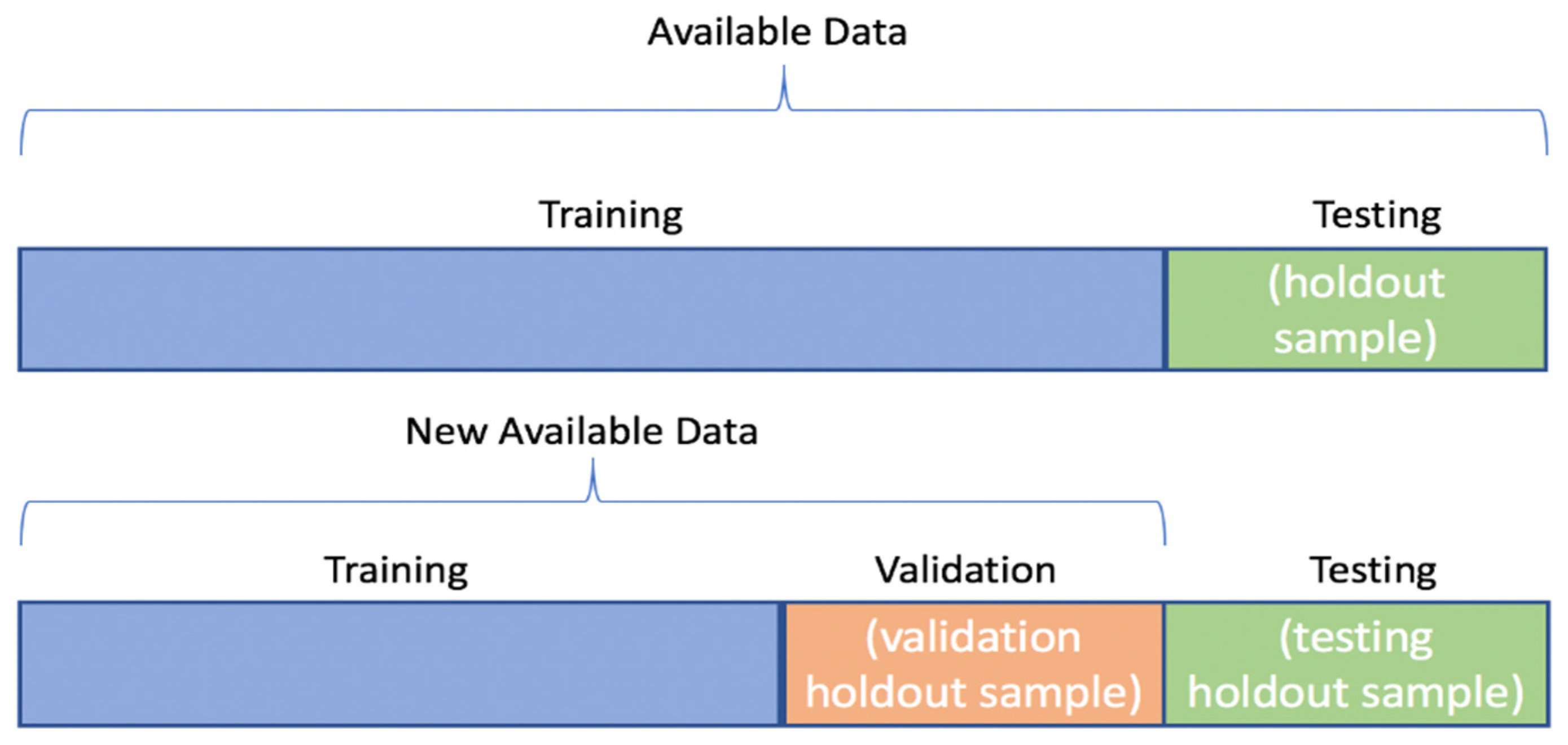
In this section, learn the dataset used and its importance for the study in terms of training and testing, in addition to the importance of utilizing influential parameters in the deep neural network. The dataset was chosen appropriately and according to the commands that are supposed to be studied here, which are right, left, forward, backward, play, stop, etc. The dataset of speech commands was chosen with a size of 3.8 GB and includes 687 audio clips for different commands. Only the English language was used in this research, and the dataset files were divided into 70% for training and 30% for testing [41], as shown in Figure 12.

Figure 12. Structure of the dataset in the proposed method.

In the standard dataset, we train the proposed model because the previous methods use the same database and for the reliability of the model. If the proposed model is efficient, then we will test the model using the proposed commands.

Each metric complements the others by addressing different aspects of model performance, from feature learning (MSE) and probabilistic predictions (Cross-Entropy) to overall effectiveness (accuracy) and specific reliability (precision). Together, they ensure a comprehensive evaluation of DNN-based speech recognition systems. It will also unify the evaluation with previous methods.

When processing data in a deep neural network, some variables must be calculated to find the accuracy in speech recognition. First, the Mean Squared Error (MSE) must be found as in the following Equation:

$$MSE={\displaystyle \frac{1}{n}}{\sum }_{i=1}^n{(y_i-{\widehat{y}}_i)}^2,$$

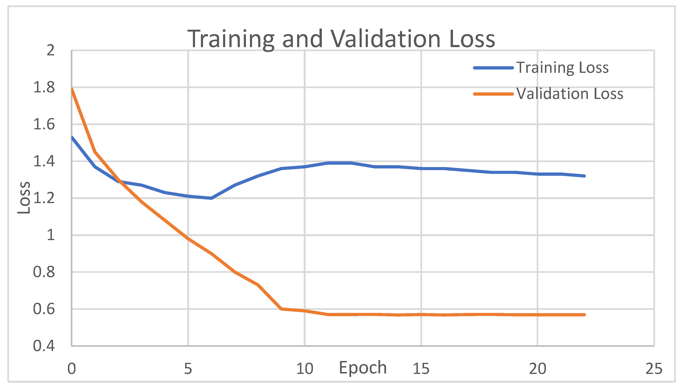
where the y is a prediction with the first round, and $\widehat{y}$ is a prediction with the last iteration. This case is for regression problems; the goal is to find continuous prediction values. Then, we have to find Cross Entropy Loss function, which means (log loss) by:

$$CEL=-{\displaystyle \frac{1}{n}}{\sum }_{i=1}^n\left[y_i\log \left({\widehat{y}}_i\right)+\left(1-y_i\right)\mathrm{l}\mathrm{o}\mathrm{g}(1-{\widehat{y}}_i)\right]$$

where n is considered as the sample number in the dataset (for certain commands) and loss function within training and validation mode, as shown in Figure 13.

Figure 13. Loss function within training and testing mode.

In classification, in general, it is important to determine the performance evaluation, and it is very useful, especially in the difference in classifications during the training phase. It is a measure of the accuracy of the work of the proposed classifier and the extent of its success. The confusion matrix, or as it is called the contingency table, measures the accuracy of the classifier through the columns that represent the predicted and the rows that represent the actual.

The accuracy can be found by the equation:

$$accuracy={\displaystyle \frac{TP+TN}{TP+FP+TN+FN}}$$

where (TP) is True Positive, (TN) is True Negative, (FP) is False Positive, and (FN) is False Negative. Precision tells us what proportion of proper path we detect and have actually found in the network and can calculated by the equation:

$$Precition={\displaystyle \frac{TP}{TP+FP}}$$

The results can be translated using the confusion matrix to be clearer and more realistic and to compare to the predicted results, as in Figure 14.

Figure 14. Confusion matrix of the proposed algorithm.

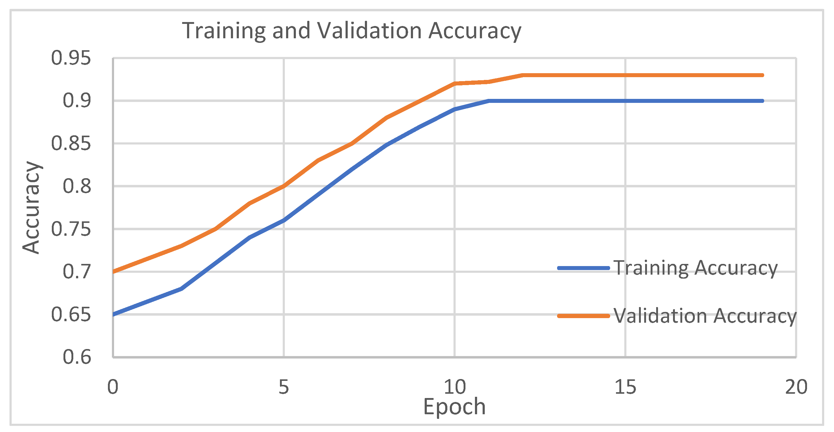
Accuracy is very important in deep learning, especially when automating the machines around us. For our research topic, the error rate should be as low as possible due to its interaction with the safety of citizens’ lives. To read accuracy more clearly, it can be described as in Figure 15. That achieves 93% and is considered good in terms of speech recognition.

Figure 15. Accuracy during training and validation mode.

The proposed technique utilizing influential parameters in deep learning significantly improves accuracy compared to existing methods Table 1. This approach ensures better adaptability to real-world scenarios, making it suitable for practical applications in driving control systems via speech recognition.

Table 1. Benchmarking with existing methods in terms of accuracy.

Approaches	Accuracy	95% Confidence Interval (±%)	Strengths	Weaknesses
Conventional ML Models [45]	85%	±2	Simple implementation	Limited feature representation
Hidden Markov Models (HMM) [46]	71%	±5	Temporal modeling	Poor generalization in noisy environments
Recurrent Neural Networks (RNN) [47]	78%	±5	Temporal dependency modeling	High computational cost
Long short-term memory (LSTM) [48]	81%	±4	Low complexity	Long time in training
Convolutional Neural Networks (CNN) [49]	83%	±3	Effective spatial feature extraction	Limited temporal modeling
Proposed	93%	±1	Robust to noise; handles variability	Requires large datasets and computational power

The proposed model combines deep learning to leverage both spatial and temporal features, as well as incorporating influential speech parameters such as pitch, tone, amplitude, etc., to improve feature representation. In this context, it shows an accuracy of 91% to 95%, with a confidence interval of 93% ± 1%, significantly outperforming existing methods illustrated in Table 1. It effectively handles dialect variation and noisy environments, such as noise, and provides real-time performance suitable for automotive interiors. On the other hand, training requires large computational resources and large datasets.

The Relationship Between Epoch, Loss, and Accuracy revolves around how the model learns and improves its performance during training. As training progresses across multiple epochs, the weights are updated using the optimization algorithm, which reflects on the values of Loss and Accuracy. It must be carefully monitored to strike a balance between good performance and avoiding overfitting.

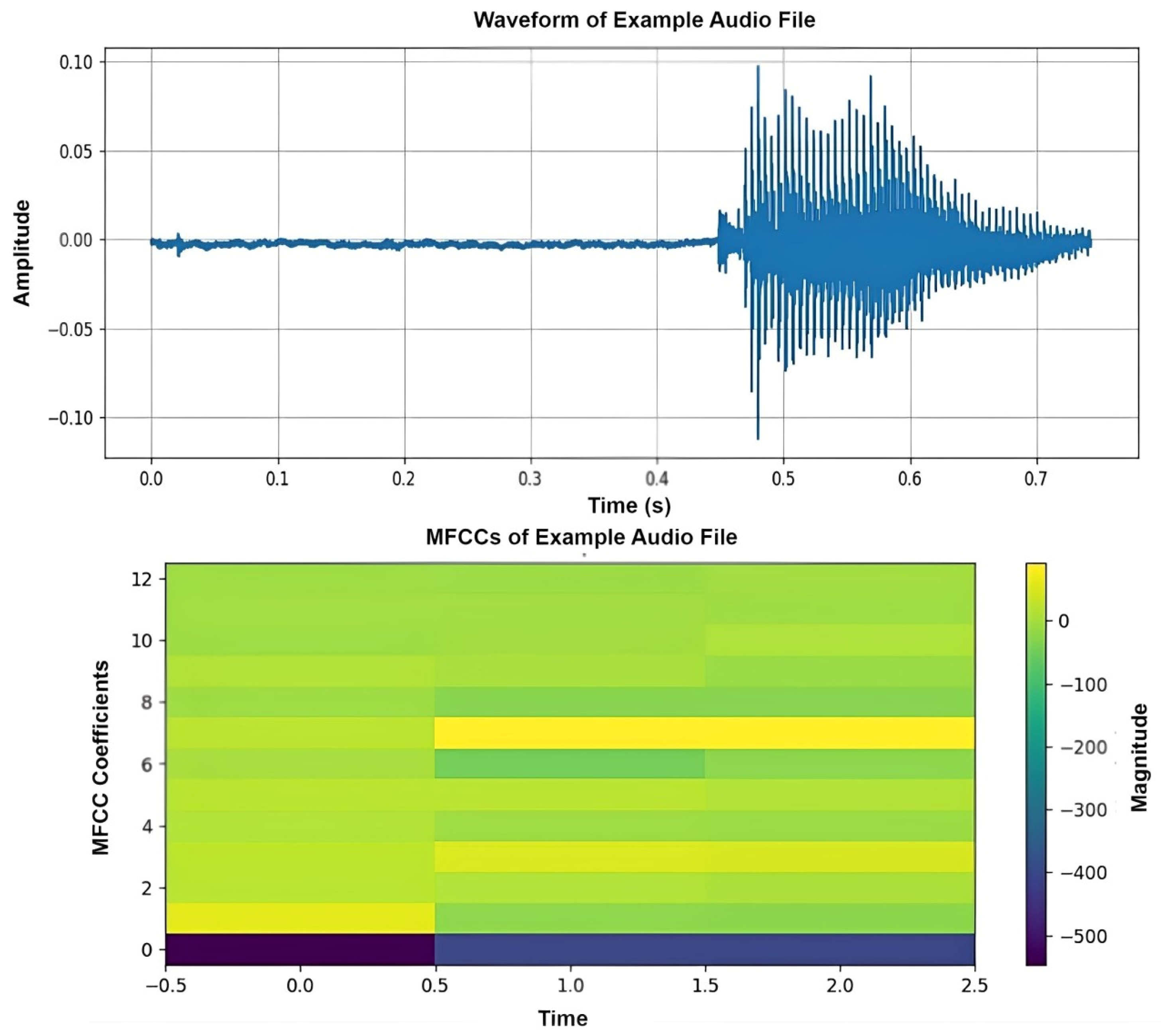
The waveform of the amplitude of any audio file, but this file differs from one command to another and from one letter to another. Also, the pronunciation of a single letter has an effect on the command and the extent of the system’s response. The accuracy is related to the amplitude that can be taken from the waveform of the file and comparing the amplitude with the remaining commands, so the progression must be calculated for each waveform, and the amplitude increases until the end of the command or word, as shown in Figure 16.

Figure 16. Waveform of a sound file extracted.

One of the important values that were calculated in our study is the Mel-frequency Cepstral coefficients, which greatly affect the knowledge of the audio file and the number of features that can be extracted from the audio file. Such features are mostly directly related to any desired accuracy in the framework of deep learning in general, as shown in Figure 17.

Figure 17. Extracting MFCC from waveform file.

The most important evaluation criterion is Peak Signal to Noise Ratio (PSNR). This metric indicates the robustness and strength of the proposed model, as it can be compared with the previous models and can be computed by finding the Mean Square Error (MSE) first and then using the equation

$$PSNR=10.{\log }_{10}{\displaystyle \frac{{Peak Value}^2 }{MSE}}$$

and expressed in decibels (dB), where the peak value is typically 2¹⁵ − 1 = 32,767. In normalize, the peak value is 1. MSE can be calculated by

$$MSE={\displaystyle \frac{1}{N}} {\sum }_{i=1}^N{({\delta }_{original}\left[i\right]-{\delta }_{processed }\left[i\right])}^2$$

For example, N is the total number of samples in the dataset. $\delta$ is the voice signal.

We can make quantitative benchmarks for more evaluation using different metrics shown in Table 2.

Table 2. Benchmarking proposed method with current studies.

Methods	Number of Languages	Environmental Effects	Size of Dataset	PSNR
A hybrid discriminant fuzzy DNN [50]	2	Automatic noise	1.4 GB (457 samples)	63 dB
MFCC and SVM in back propagation model [51]	1	artificial noise embedded	905 MB (278 Samples)	71 dB
Hybrid CTC/RNN-T in visual audio [52]	3	Automatic noise	1.10 GB (307 mixed sample)	47 dB
Modified Weighted-KNN with different environments [53]	3	Natural noise and distortion	Big dataset (unknown)	61 dB
Proposed	1	Automatic noise	3.8 GB (687 samples)	78 dB

5. Conclusion and Limitations

Deep learning is a scalable technology, so it has been used in driving control to ensure safety and rapid response. The proposed method has proven its worth by integrating deep neural network technology into speech control and achieved 93% accuracy, which confirms the ability of the proposed model to interpret and execute voice commands. The average response time was 0.75 s with loud sounds, which led to ease of use and reliability. The approach has shown an improvement in accuracy by 15% and in response time by 20%. Future studies may focus on expanding the set of commands and data in general, and user devices may be enhanced by integrating additional sensors to develop models. This study focused on the potential of deep learning in speech recognition to improve driving control systems and ensure greater efficiency and safety in driving.

In our study, there are several limitations to take into consideration. Speech recognition requires a large and diverse training dataset due to the different languages and dialects. This can have limited bias. Such models are often sensitive to noise, which leads to some movements and spoken symbols being replaced outside the vocabulary. Discrimination-based systems often need to operate in real-time due to the sensitivity of the environment in which they operate.