Dynamic Risk Assessment of Wind Farms Under Extreme Gust Disturbances Using BiLSTM, Adaboost, and Adaptive Kernel Density Estimation for Enhanced Prediction

Abstract

Under extreme gusty weather conditions, wind power output fluctuates significantly, and the operational risks of wind farms exhibit strong randomness and complexity. Addressing the issue of limited sample data under such extreme wind speed conditions, which leads to low accuracy in risk assessment, this study proposes a multi-dimensional risk assessment method for wind farms based on the BiLSTM-Adaboost-ABKDE algorithm framework and ITA-TPW (Integrated Trend Analysis—Time-Series Probability Weighting) weighted fusion. First, a wind farm operational risk assessment model based on a multi-dimensional risk indicator system is constructed to assess the impact of these extreme weather conditions on wind farm operational risks. Second, to enhance the robustness of wind power output prediction under small-sample conditions, a BiLSTM (Bidirectional Long Short-Term Memory) network is introduced to capture the bidirectional temporal dependencies of wind power output. Through the Adaboost weighted ensemble of sub-models, combined with the ABKDE (Adaptive Bandwidth Kernel Density Estimation) algorithm for probability density estimation of prediction outputs, high-precision point prediction and uncertainty quantification are unified. Furthermore, we combine trend analysis sensitivity analysis using the ITA method with time-series probability weighting using the TPW method to assess key risks such as voltage overlimit, power flow overlimit, and load imbalance in wind farms under extreme wind speeds from multiple perspectives. The dataset used in this study comes from Hebei Province, covering wind power data from 1 March 2020 to 31 May 2023, and the simulation platform used is MATLAB R2023a. Simulation analysis was conducted using the IEEE RTS-79 node system to validate the effectiveness of the proposed method. The results showed that the proposed method improved the accuracy of load shedding risk and voltage overlimit risk indicators by 6.15% and 4.79%, respectively. Additionally, the reliability of the system’s comprehensive risk indicators was significantly enhanced, validating the effectiveness of this method in improving the accuracy and reliability of operational risk assessment for wind farms under extreme weather conditions.

1. Introduction

With the intensification of global climate change, the frequency of extreme weather events, especially strong winds and abrupt wind speed changes, has been increasing. These extreme weather phenomena often lead to voltage fluctuations, power flow interruptions, and load imbalances in the power grid, seriously threatening the safety and stability of the grid. Wind power generation is highly sensitive to wind speed, particularly under extreme weather conditions. When wind turbines are disconnected on a large scale, the accuracy of wind power forecasting can significantly decline [1,2]. This issue not only increases the complexity of grid scheduling but also affects the stable operation of the grid. Therefore, finding an effective method to improve wind power forecasting accuracy under extreme wind conditions and conducting precise risk assessments is crucial for ensuring grid stability and safety [3,4,5,6].

In recent years, researchers have begun to adopt data decomposition methods to preprocess wind power data to improve forecasting accuracy. These methods can effectively capture the nonlinear features in the data and adapt to dynamic changes, thereby reducing the complexity of power sequences and improving forecasting accuracy [7]. For example, EMD (Empirical Mode Decomposition) [7] and CEEMD (Complementary Ensemble Empirical Mode Decomposition) [8] have been widely used in wind power forecasting, but they still face issues such as mode mixing and high computational complexity. VMD (Variational Mode Decomposition), as an emerging method, can effectively handle high-frequency noise and non-stationary signals, making it a hot topic in current data processing research [9]. However, under extreme weather conditions, the scarcity of wind power data limits forecasting models in terms of parameter setting and hypothesis testing, making it difficult to capture the instantaneous nonlinear features of wind power, which affects the training and prediction performance of the models.

To address the issue of reduced forecasting accuracy caused by small sample sizes under extreme weather events, some studies have proposed data augmentation techniques. For example, in the literature, ref. [10] proposed several data sampling strategies to solve the problem of imbalanced training samples under different weather events, effectively improving the accuracy of wind power ramp-up warnings. Literature [11,12] proposed data augmentation methods based on Generative Adversarial Networks (GAN) to expand training samples for wind power, thereby improving the accuracy of short-term wind power forecasting. At the same time, Conditional Generative Adversarial Networks (CGAN) and TimeGAN have also been applied to augment small sample data, achieving good forecasting results [13,14]. Despite these advancements, existing data augmentation methods still fail to fully preserve the physical characteristics and temporal dependencies of wind power data. Therefore, traditional modal decomposition algorithms still face challenges when handling the transient nonlinear dynamic features of wind power under extreme weather, such as insufficient multi-scale feature decoupling and sensitivity to parameter settings, which leaves room for improving the physical interpretability and accuracy of these methods.

To address these issues, this paper proposes a hybrid model based on Bidirectional Long Short-Term Memory (BiLSTM)—Adaptive Boosting (AdaBoost)—Adaptive Bandwidth Kernel Density Estimation (ABKDE). This model combines BiLSTM’s powerful temporal modeling capabilities, AdaBoost’s sample weighting mechanism, and the uncertainty quantification of the ABKDE module to solve the small sample and high volatility issues in extreme gust data. BiLSTM is used to extract temporal features from wind speed data, while AdaBoost optimizes the training process and enhances the recognition ability for hard-to-predict samples. The ABKDE module performs non-parametric probability density estimation on prediction residuals, transforming traditional “point predictions” into “prediction + uncertainty,” effectively improving both prediction accuracy and uncertainty quantification. In extreme gust scenarios with limited historical samples and strong noise, this hybrid structure allows BiLSTM to capture bidirectional temporal dependencies, while AdaBoost emphasizes hard-to-predict extreme ramps during training and ABKDE provides a noise-robust probabilistic description of prediction errors, thereby directly targeting the coexistence of small sample size and high volatility. Similar hybrid models have achieved significant success in other fields. For example, Gong Wenjie et al. [15] combined BiLSTM with AdaBoost to extract temporal features via BiLSTM and adjusted sample weights using AdaBoost, improving the accuracy and robustness of heat load forecasting. Zhang Yushan et al. proposed a BiLSTM–AdaBoost model combined with Bayesian optimization, which extracted features from time-series data using BiLSTM and optimized multi-model prediction performance via AdaBoost, significantly improving short-term heat load forecasting accuracy, especially in the face of data fluctuations and noise [16]. However, these BiLSTM–AdaBoost models were developed for relatively smooth load or time-series data with abundant historical samples; when directly applied to rare, high-amplitude gust events, their ensemble averaging effect tends to smooth sharp power ramps and underrepresent tail behavior, which limits their applicability to operational risk analysis under extreme gust disturbances.

In addition, Yang Tengjie et al. [17] proposed an interpretable model based on NRBO-XGBoost and ABKDE, using ABKDE for error correction and successfully improving tunneling speed prediction accuracy. Kang Yan et al. [18] proposed a flood interval forecasting method based on an error correction fusion model, which successfully improved forecast accuracy by combining error correction with ABKDE. These studies demonstrate that the combination of BiLSTM–AdaBoost and ABKDE has significant advantages in feature extraction and time-series analysis, providing strong theoretical support for this study.

In recent years, modern deep learning technologies such as Generative Adversarial Networks (GAN) and Transformer have been introduced into the fields of extreme weather event prediction and wind power forecasting. For example, in the literature, ref. [19] proposed a hybrid model that combines gust detection with a Conditional LSTM to more accurately forecast wind speed under extreme gust conditions. However, these methods mainly focus on improving wind speed or wind power forecasting performance and do not explicitly consider how real-time wind power disturbances propagate to grid-level operational risks. Similarly, Li Ling et al. [20] proposed a wind farm fault and capacity loss prediction method based on ensemble learning, which provides an important reference for wind power grid integration risk assessment. Nevertheless, most of these approaches are still confined to a single link in the chain and fail to comprehensively cover the full process from “extreme wind speed disturbances” through “wind power forecasting” to “grid operation risk assessment.”

Motivated by these limitations, this study applies the BiLSTM–AdaBoost–ABKDE hybrid model to wind power forecasting and grid risk assessment, aiming to improve forecasting accuracy while quantifying uncertainty, thereby providing a new solution for wind power grid scheduling and risk assessment under extreme gust conditions. Compared with existing hybrid and ensemble forecasting methods that mainly focus on point prediction accuracy under normal or moderately fluctuating conditions, or address only one stage of the process, the proposed framework explicitly targets extreme gust disturbances with scarce data and couples wind power forecasting with multi-dimensional operational risk indicators for wind farms and the power grid. To evaluate this framework on a realistic yet standardized benchmark, the IEEE RTS-79 reliability test system is adopted as the background network, providing representative topology, generation, and load data for reproducible dynamic risk assessment under extreme gust conditions.

2. Precise Modeling of Wind Farms Under Extreme Gusts

2.1. Detailed Wind Farm Model

2.1.1. Extreme Wind Event Model

Extreme wind conditions refer to wind conditions with a frequency of once per year that affect the operational safety of wind turbines during operation, as well as those with a frequency of once per 50 years that affect the survival status of wind turbines. Table 1 presents the wind turbine classes and their parameters according to the IEC 61400-1 standard [21].

Table 1. Parameters for Wind Turbine Classifications.

Fan Class	Ⅰ	Ⅱ	Ⅲ	S
$V_{\mathrm{r}\mathrm{e}f}(m/s)$	50	42.5	37.5	Designer-specified value
$V_{\mathrm{ave}}(m/s)$	10	8.5	7.5
$AIref(-)$	0.18	0.18	0.18
$a(-)$	2	2	2
$BIref(-)$	0.16	0.16	0.16
$a(-)$	3	3	3

Note (1): $V_{\mathrm{r}\mathrm{e}f}(m/s)$ represents the 10 min reference average wind speed. Note (2): $V_{\mathrm{ave}}(m/s)$ represents the historical average wind speed at hub height. Note (3): $AIref(-)$ and $BIref(-)$ are the reference turbulence intensities at a mean wind speed of 15 m/s for turbulence classes A and B, respectively. Note (4): $a(-)$ is the wind shear exponent used to describe the vertical wind speed profile.

(1) Extreme wind speed model: sustained wind model or turbulent wind model. Extreme wind speed models are based on reference wind speeds and specific turbulent standard deviations [22].

50-year return period extreme average wind speed:

$$V_{e50}=1.4V_{ref}{({\displaystyle \frac{z}{z_{hub}}})}^{0.11}$$

(1)

1-year return period extreme average wind speed:

$$V_{e1}=0.8V_{e50}$$

(2)

Longitudinal turbulent standard deviation:

$${\sigma }_1=0.11V_{\mathrm{hub}}$$

(3)

(2) Extreme operational gust model: Amplitude of gusts at the hub of a standard wind turbine:

$$V_{gust}=\min \left[1.35\left(V_{e1}-V_{hub}\right),3.3\left({\displaystyle \frac{{\sigma }_1}{1+0.1D/A_1}}\right)\right]$$

(4)

where D is the rotor diameter; Wind speed:

$$V(z,t)=\left\{\begin{array}{ll}V(z)-0.37V_{gust}\sin \left({\displaystyle \frac{3\pi t}{T}}\right)\left(1-\cos \left({\displaystyle \frac{2\pi t}{T}}\right)\right),\hfill & 0\le t\le T\hfill \\ V(z),\hfill & \mathrm{Others}\hfill \end{array}\right.$$

(5)

where the 1-year return period extreme operational gust T is taken as 10.5 s, and the 50-year return period T is taken as 14 s.

(3) Extreme Continuous Gust Model:

$$V(z,t)=\left\{\begin{array}{ll}V(z),\hfill & t\le 0\hfill \\ V(z)+0.5V_{cg}\left(1-\cos \left({\displaystyle \frac{\pi t}{T}}\right)\right),\hfill & 0\le t\le T\hfill \\ V(z)+V_{cg},\hfill & t>T\hfill \end{array}\right.$$

(6)

The amplitude of extreme continuous gusts for standard wind turbine classes is 15 m/s, with T = 10 s, representing the rise time.

(4) Extreme continuous gust model with wind direction change: The angle of wind direction change for extreme continuous gusts is within [0°, ${\theta }_{cg}$], where

$${\theta }_{cg}=\left\{\begin{array}{ll}{180}^{°},\hfill & V_{hub}\le 4 \mathrm{m}/\mathrm{s}\hfill \\ {\displaystyle \frac{{720}^{°}}{V_{hub}}},\hfill & 4 \mathrm{m}/\mathrm{s}<V_{hub}<V_{ref}\hfill \end{array}\right.$$

(7)

Additionally, the relationship between wind direction and time is:

$${\theta }_{cg}=\left\{\begin{array}{ll}\pm 0.5{\theta }_{cg}\left(1-\cos \left({\displaystyle \frac{\mathsf{\Pi }t}{T}}\right)\right),\hfill & t<0\hfill \\ \pm {\theta }_{cg},\hfill & 0\le t\le T\hfill \\ \pm {\theta }_{cg},\hfill & t>T\hfill \end{array}\right.$$

(8)

where the duration of wind direction change T is taken as 6 s, and the sign (+ or −) should be selected based on the better transient load. The wind direction is considered unchanged after the transient extreme wind direction change ends.

(5) Extreme wind direction change:

$${\theta }_e=\pm 4\arctan \left({\displaystyle \frac{{\sigma }_1}{V_{hub}\left(1+0.1D/A_1\right)}}\right)$$

(9)

The amplitude of the extreme wind direction change is where D is the rotor diameter; the value is within the range [−180°, 180°];

The function of extreme wind direction with respect to time:

$$\theta (t)=\left\{\begin{array}{ll}\pm 0.5{\theta }_e\left(1-\cos \left({\displaystyle \frac{\mathsf{\Pi }t}{T}}\right)\right),\hfill & t<0\hfill \\ {\theta }_e,\hfill & 0\le t\le T\hfill \\ {\theta }_e,\hfill & t>T\hfill \end{array}\right.$$

(10)

(6) Extreme wind shear: The transient wind speed values of extreme wind shear are divided into transient vertical shear and transient horizontal shear.

Transient vertical shear:

$$V(z,t)=\left\{\begin{array}{ll}{V}_{hub}{\left({\displaystyle \frac{z}{z_{hub}}}\right)}^{\alpha }\pm {\displaystyle \frac{z-z_{hub}}{D}}\left(\left(2.5+0.2\beta {\sigma }_1{\left({\displaystyle \frac{D}{A_1}}\right)}^{1/4}\right)\left(1-\cos \left({\displaystyle \frac{2\mathsf{\Pi }t}{T}}\right)\right)\right),\hfill & 0\le t\le T\hfill \\ V_{hub}{\left({\displaystyle \frac{z}{z_{hub}}}\right)}^{\alpha },\hfill & \mathrm{Others}\hfill \end{array}\right.$$

(11)

Transient horizontal shear:

$$b(y,z,t)=\left\{\begin{array}{ll}{V}_{nub}{\left({\displaystyle \frac{z}{z_{nub}}}\right)}^{\alpha }\pm {\displaystyle \frac{z-z_{nub}}{D}}\left(\left(2.5+0.2\beta {\sigma }_1{\left({\displaystyle \frac{D}{A_1}}\right)}^{1/4}\right)\left(1-\cos \left({\displaystyle \frac{2\mathsf{\Pi }t}{T}}\right)\right)\right),\hfill & 0\le t\le T\hfill \\ V_{nub}{\left({\displaystyle \frac{z}{z_{nub}}}\right)}^{\alpha },\hfill & \mathrm{Others}\hfill \end{array}\right.$$

(12)

In Equations (11) and (12), a = 0.2, β = 0.64, T = 12 s; D is the diameter of the wind wheel.

To illustrate the parameter ranges adopted in this paper and to validate the physical reasonableness of Equations (4), (11) and (12), we consider a representative IEC Class II wind turbine. According to Table 1, the corresponding 10 min reference mean wind speed is 37.5–42.5 m/s, and the hub-height mean wind speed under normal operation is approximately 10–15 m/s. In our simulations, the rotor diameter D of the turbines installed in the wind farm lies in the range of 80–100 m, and we take D = 90 m as a representative value for calculating the extreme gust and transient shear profiles.

For a hub-height mean wind speed of 15 m/s and D = 90 m, substituting the above parameters into Equations (11) and (12) yields transient vertical and horizontal shear components whose maximum increments are on the order of 1.5–2.0 m/s across the rotor disk, i.e., approximately 10–15% of the hub-height mean wind speed.

2.1.2. Extreme Gust Duration Model

Assessing the impact intensity of extreme weather on power systems requires consideration of both spatial and temporal dimensions. Spatially, system components operate under varying conditions depending on their geographic locations. Temporally, exposure duration differs across affected areas. As shown in Figure 1, the intersection of the extreme weather trajectory with the spatial layout of the power system determines exposure time, which is governed by the event’s path length and propagation speed, as expressed in Equation (13).

$$T_{len}={\displaystyle \frac{D_{wr}}{V_w}}$$

(13)

Figure 1. Schematic diagram of the spatial relationship between extreme weather trajectories and the affected power system area.

In Equation (13), $D_{wr}$ is the trajectory distance of extreme gusts in the affected power system area, and $V_w$ is the movement speed of the center of extreme gusts in this area.

Figure 2 provides a schematic illustration of how the trajectory of an extreme gust event leads to different exposure durations for different wind farms. The gust propagates along the dashed path with a translational velocity $V_w$, and its influence area at each time instant is represented by the moving circular footprint with radius $D_{wr}$ around the gust center. As shown in the figure, the trajectory intersects the influence region of Wind Farm 1 over a longer chord length than that of Wind Farm 2. According to Equation (13), Wind Farm 1 experiences a longer exposure duration, while Wind Farm 2 is exposed for a shorter period.

Figure 2. Extreme gust trajectory and exposure regions of wind farms. The dashed line represents the path of extreme wind gusts, and the arrows indicate the diameter of the circle, which is the parameter Dwr.

2.1.3. Wind Energy Conversion Model

Based on extensive research [23], the output power of wind turbines satisfies a specific relationship curve with wind speed, known as the wind turbine power characteristic curve. A typical wind turbine power characteristic curve is shown in Figure 3.

Figure 3. Wind turbine power curve.

In the figure, $v_{ci}$ represents the cut-in wind speed, $v_{co}$ represents the cut-out wind speed, $v_r$ represents the rated wind speed, $P_{wr}$ represents the active power generated by the wind turbine at the rated wind speed, and $v$ represents the wind speed at the wind farm. According to the principles of aerodynamics, the electrical power generated by a wind turbine is proportional to the cube of the wind speed. The relationship between the output power and the wind speed can be expressed as:

$$P_W(v_x)=\left\{\begin{array}{ll}0,\hfill & (v_x<v_{ci})\cup (v_x>v_{co})\hfill \\ {\displaystyle \frac{P_{wr}}{v_r^3-v_{ci}^3}}\left(v_x^3-v_{ci}^3\right),\hfill & (v_{ci}\le v_x\le v_r)\hfill \\ P_{wr},\hfill & (v_r<v_x\le v_{co})\hfill \end{array}\right.$$

(14)

In Equation (14), $P_W(v_x)$ represents the active power generated by the $v_x$ fan under wind speed.

In this study, the wind turbines installed in the case study wind farm have operating parameters $v_{ci}$ = 3 m/s, $v_r$ = 12 m/s, and $v_{co}$ = 25 m/s, according to the manufacturer’s technical specifications, and these values are used consistently in all simulations when applying the power curve in Equation (14).

3. BiLSTM-Adaboost-ABKDE Algorithm

To address the challenges posed by small sample sizes, high volatility, and high uncertainty in wind power forecasting under extreme gust conditions, this paper proposes a BiLSTM-Adaboost-ABKDE hybrid prediction framework. In contrast to deep learning models that rely on large sample sizes for training, such as Transformer or GAN, the proposed approach emphasizes model robustness, generalization capability, and computational efficiency.

BiLSTM (Bidirectional Long Short-Term Memory) networks are capable of modeling both forward and backward dependencies in time series data, effectively capturing the nonlinear dynamic features induced by wind speed fluctuations [24]. Studies have demonstrated that BiLSTM achieves higher accuracy and stability compared to unidirectional LSTM and GRU in small-sample renewable energy forecasting. To mitigate the interference of noisy samples and non-stationary signals during training, this paper employs the Adaboost ensemble algorithm, which integrates multiple BiLSTM sub-models [25].

In this study, the ABKDE (Adaptive Bandwidth Kernel Density Estimation) module is utilized to model the probability distribution of the residuals between the BiLSTM predicted values and the actual values. Specifically, BiLSTM generates wind speed forecasts through its temporal modeling capabilities, while Adaboost enhances the model’s performance by weighting multiple BiLSTM models. Subsequently, ABKDE estimates the probability density of these prediction residuals, thereby quantifying the uncertainty in the model’s predictions. Compared to traditional KDE methods, ABKDE offers the advantage of adaptively adjusting the bandwidth parameter based on local data density, resulting in more precise and smoother distribution estimates. This adaptive mechanism is particularly crucial in small-sample environments, ensuring that prediction errors’ uncertainty is accurately quantified, thus providing more reliable information for risk assessment.

Although models such as Transformer and GAN perform well on large datasets [26], their reliance on large sample sizes and high computational resources limits their application in small-sample and high-noise data scenarios. In contrast, the BiLSTM-Adaboost-ABKDE framework exhibits superior convergence stability and prediction accuracy in small-sample, high-noise wind power data scenarios. Additionally, it effectively quantifies prediction uncertainty, further enhancing grid risk assessment capabilities.

3.1. BiLSTM Algorithm Principle

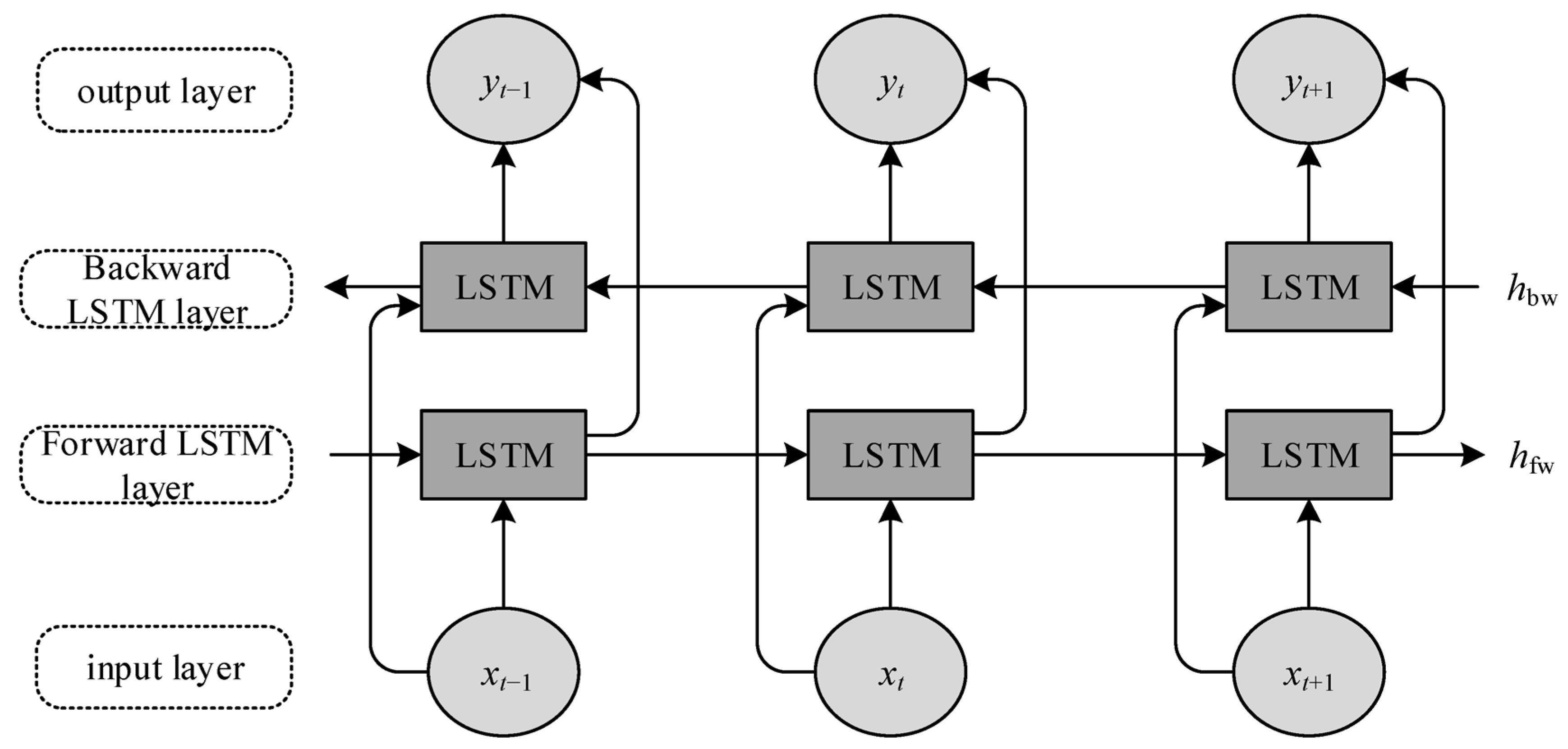
The bidirectional long short-term memory network is based on LSTM and captures bidirectional dependencies in time series by combining the outputs of the forward and backward LSTM networks, thereby improving the accuracy of model predictions to a certain extent. The BiLSTM algorithm structure is shown in Figure 4 [24].

Figure 4. BiLSTM algorithm structure.

Specific expression of the BiLSTM algorithm:

$$\begin{array}{l}\overrightarrow{h_t}=LSTM(x_t,\overrightarrow{h_{t-1}})\\ \overleftarrow{h_t}=LSTM(x_t,\overleftarrow{h_{t-1}})\\ y_t=\sigma \left(W_y\left[\overrightarrow{h_t},\overleftarrow{h_t}\right]+b_y\right)\end{array}$$

(15)

In Equation (15), $\overrightarrow{h_t}$ is the state of the forward LSTM hidden layer at time t; $\overleftarrow{h_t}$ is the state of the backward LSTM hidden layer at time t; $W_y$ represents the weight; $b_y$ represents the bias term; $x_t$ represents the input data at time t; $y_t$ represents the output data at time t.

3.2. Adaboost Algorithm Principle

Adaboost is an ensemble learning algorithm that iteratively builds multiple weak regressors and aggregates them into a strong predictor [27]. At each iteration, training sample weights are updated, assigning greater importance to observations with larger previous errors. The reweighted data are used to train the next weak regressor, and the final model is obtained by combining all weak regressors.

The Adaboost training procedure is as follows:

(1)

The initial weight distribution of the training data samples, i.e., assigning an initial weight to each training sample.

$$D_1=⟨w_{11},\cdots ,w_{1i},\cdots ,w_{1N}⟩,\hspace{1em}{w}_{1i}={\displaystyle \frac{1}{N}},\hspace{1em}i=1,2,\cdots ,N$$

(16)

(2)

For t = 1, 2, 3, …, T, perform weight adjustment according to the following steps.

First, when training the tth weak predictor, train the training set containing the weight distribution and obtain the weak predictor $G_t(\mathrm{x})$.

Second, calculate the total prediction error Et for each weak predictor.

$$e_t={\displaystyle \sum _{i=1}^N{D}_t^i}{e}_t^i=P\left(\left|{\displaystyle \frac{G_t(x_i)-y_i}{y_i}}\right|>\phi \right)$$

(17)

In the formula: $G_t(\mathrm{x})$ is the predicted output; $y_i$ is the expected output; $\phi$ is the set threshold.

Third, based on the calculated error and the weight coefficient ${\alpha }_t$ of the current weak classifier:

$${\alpha }_t={\displaystyle \frac{1}{2}}\log {\displaystyle \frac{1-e_t}{e_t}}$$

(18)

Fourth, update the weight distribution of the training set:

$$\left\{\begin{array}{l}{D}_{t+1}=\left(w_{t+1,1},\dots ,w_{t+1,j},\dots ,w_{t+1,N}\right)\hfill \\ w_{t+1,i}={\displaystyle \frac{w_{ti}}{Z_t}}{e}^{-{\alpha }_t{y}_i{G}_t(x_i)},Z_t={\displaystyle \sum _{i=1}^N{\omega }_{ti}}{e}^{-{\alpha }_t{y}_i{G}_t(x_i)}\hfill \end{array}\right.$$

(19)

In the formula: $Z_t$ is the normalization factor.

(3)

Finally, construct a linear combination of T weak predictors to form a strong predictor.

$$G(x)=\mathrm{sign}(f(x))=\mathrm{sign}\left({\displaystyle \sum _{t=1}^T{\alpha }_t}{G}_t(x)\right)$$

(20)

3.3. ABKDE Algorithm Principle

Kernel density estimation (KDE) is a nonparametric method for estimating the probability density function (PDF) of a random variable from observed data. It assigns a kernel function—such as Gaussian or Epanechnikov—to each data point, sums their contributions, and produces a smooth estimate of the underlying distribution.

KDE depends on two parameters: the kernel function, which defines local influence, and the bandwidth, which controls the degree of smoothing. Small bandwidths may lead to overfitting by capturing noise, whereas large bandwidths may oversmooth and obscure important features.

In addition to marginal density estimation, KDE can estimate joint PDFs, enabling conditional density analysis and quantile-based inference. This capability supports evaluating predictor effects across the distribution and constructing smooth quantile regression curves without strict parametric assumptions.

For KDE-based quantile regression, kernel and bandwidth parameters are typically optimized using cross-validation to capture conditional structures effectively.

The general formula for KDE is:

$$f_h(x)={\displaystyle \frac{1}{nh}}{\displaystyle \sum _{i=1}^{n}K}\left({\displaystyle \frac{x-x_i}{h}}\right)$$

(21)

In the formula: $x_1$, $x_2$, …, $x_{\mathrm{n}}$ are sample data; $K(·)$ is the kernel function; $h$ is the bandwidth parameter.

There are many types of KDE kernel functions, and the following are commonly used:

(1)

Gaussian kernel function:

$$K(x)={\displaystyle \frac{1}{\sqrt{2\pi }}}\exp \left(-{\displaystyle \frac{x^2}{2}}\right)$$

(22)

(2)

Trigonometric kernel function:

$$K(x)=(1-|x|)I(|x|\le 1)$$

(23)

(3)

Epanechnikov kernel function:

$$K(x)={\displaystyle \frac{3}{4}}(1-x^2)I(|x|\le 1)$$

(24)

This study adopts an adaptive bandwidth strategy to enhance kernel density estimation (KDE) accuracy. Unlike traditional fixed-bandwidth KDE, which applies a uniform smoothing parameter to all observations, the adaptive approach adjusts the bandwidth according to local data density [28]. Specifically, bandwidth is defined as a function of the estimated density at each observation: smaller values are applied in dense regions to capture fine-scale variations, while larger values are used in sparse regions to maintain smoothness and reduce variance. This locally adaptive mechanism yields a more accurate representation of the underlying probability density function.

By alleviating over-smoothing in dense areas and overfitting in sparse areas, adaptive bandwidth KDE provides a robust, data-sensitive framework for nonparametric density estimation [29].

3.4. BiLSTM-Adaboost-ABKDE Algorithm Process

(1)

Data Preparation and Preprocessing:

To account for the temporal characteristics and environmental variability inherent in wind power data, systematic preprocessing is first applied to the raw dataset. In this study, Z-score standardization is employed to normalize environmental variables—such as wind speed and temperature—thereby eliminating dimensional disparities and facilitating subsequent model training and analysis.

$$X_{\mathrm{std}}={\displaystyle \frac{X-\mu }{\sigma }}$$

(25)

where $X$ is the original data, $\mu$ is the mean of the feature, and $\sigma$ is the standard deviation.

To better capture the nonlinear characteristics and periodic variations in wind power, the model incorporates not only the original features such as wind speed and temperature, but also the cube of wind speed, the sine and cosine components of wind direction, and time-lagged features. Furthermore, recursive feature elimination is employed to select the most predictive subset of these features.

On this basis, the sliding window method is used to construct time series samples. The historical window length L and prediction step length H are defined, and the time series data is converted into an L × d-dimensional input matrix and an H-dimensional output vector, which facilitates training of the BiLSTM model:

$$X_t=\left[F_{t-L},F_{t-L+1},\dots ,F_{t-1}\right]$$

(26)

$$Y_t=\left[P_t,P_{t+1},\dots ,P_{t+H-1}\right]$$

(27)

(2)

Time Series Data Modeling:

The bidirectional long short-term memory (BiLSTM) network is an extension of the conventional LSTM architecture, designed to capture both past and future context within sequential data. In the context of wind power forecasting, BiLSTM is particularly effective in modeling long-term temporal dependencies, thereby enhancing prediction accuracy.

Specifically, BiLSTM employs two separate LSTM units. The forward LSTM processes the input sequence in chronological order, capturing information from the current and preceding time steps:

$$\overrightarrow{h_t}=\sigma \left(W_{\overrightarrow{f}}·\left[x_t,\overrightarrow{h_{t-1}}\right]+b_{\overrightarrow{f}}\right)$$

(28)

The other is a backward LSTM unit, which processes the input sequence at the current moment and thereafter:

$$\overleftarrow{h_t}=\sigma \left(W_{\overleftarrow{f}}·\left[x_t,\overleftarrow{h_{t+1}}\right]+b_{\overleftarrow{f}}\right)$$

(29)

Ultimately, the two are fused through a hyperbolic tangent activation function to form the final feature representation:

$$h_t=\tanh \left(W_f·\left[\overrightarrow{h_t},\overleftarrow{h_t}\right]\right)$$

(30)

(3)

Ensemble Learning and Accuracy Enhancement:

Within the BiLSTM-Adaboost framework, Adaboost integrates the outputs of multiple BiLSTM submodels through a weighted combination to produce the final prediction. Each BiLSTM submodel is trained with a focus on different subsets of the data at various stages, allowing the ensemble to capture diverse patterns and reduce prediction error. The aggregation of multiple submodels enhances robustness and improves overall forecasting accuracy.

Specifically: First, calculate the weighted average absolute error of the current model:

$${ϵ}_t={\displaystyle \frac{{\displaystyle \sum _{i=1}^N{D}_t}(i)·|y_i-{\widehat{y}}_i|}{{\displaystyle \sum _{i=1}^N{D}_t}(i)}}$$

(31)

Then calculate the submodel weights based on the error rate:

$${\alpha }_t=0.5\ln \left({\displaystyle \frac{1-{ϵ}_t}{{ϵ}_t}}\right)$$

(32)

Final update sample weight:

$$D_{t+1}(i)={\displaystyle \frac{D_t(i)·\exp ({\alpha }_t|e_i|)}{Z_t}}$$

(33)

where $Z_t$ is the normalization factor.

(4)

Uncertainty modeling and probability density estimation:

After obtaining the integrated point prediction values, the ABKDE algorithm constructs an uncertainty model based on the training set prediction error samples: let $y_t$ denote the actual wind power at time t and ${\stackrel{\wedge }{y}}_t$ denote the corresponding integrated point prediction of the BiLSTM-Adaboost model; the prediction error is computed as $e_t$ = $y_t$ − ${\stackrel{\wedge }{y}}_t$, and the sample set {$e_t$ for t = 1, …, N} is used as the input to the ABKDE procedure in Equations (34)–(36).

$$h_0=1.06{\widehat{\sigma }}_e{N}^{-0.2}$$

(34)

Then estimate the local density factor for each sample point:

$$h_i=h_0{\lambda }_i^{\beta }$$

(35)

Next, calculate the adaptive bandwidth, and finally use the Gaussian kernel function to generate the probability density function:

$$\widehat{f}(p)={\displaystyle \frac{1}{N}}{\displaystyle \sum _{i=1}^N\frac{1}{h_i}}K\left({\displaystyle \frac{p-\widehat{p}-e_i}{h_i}}\right)$$

(36)

The BiLSTM-Adaboost-ABKDE algorithm ultimately outputs a sequence of predicted wind power values for the next H time steps and their probability density distribution:

$$\widehat{Y}=\left[{\widehat{P}}_t,{\widehat{P}}_{t+1},\dots ,{\widehat{P}}_{t+H-1}\right]$$

(37)

$${\widehat{f}}_P(p)={\displaystyle \frac{1}{N}}{\displaystyle \sum _{i=1}^N\frac{1}{h_i\sqrt{2\pi }}}\exp \left(-{\displaystyle \frac{1}{2}}{\left({\displaystyle \frac{p-\widehat{p}-e_i}{h_i}}\right)}^2\right)$$

(38)

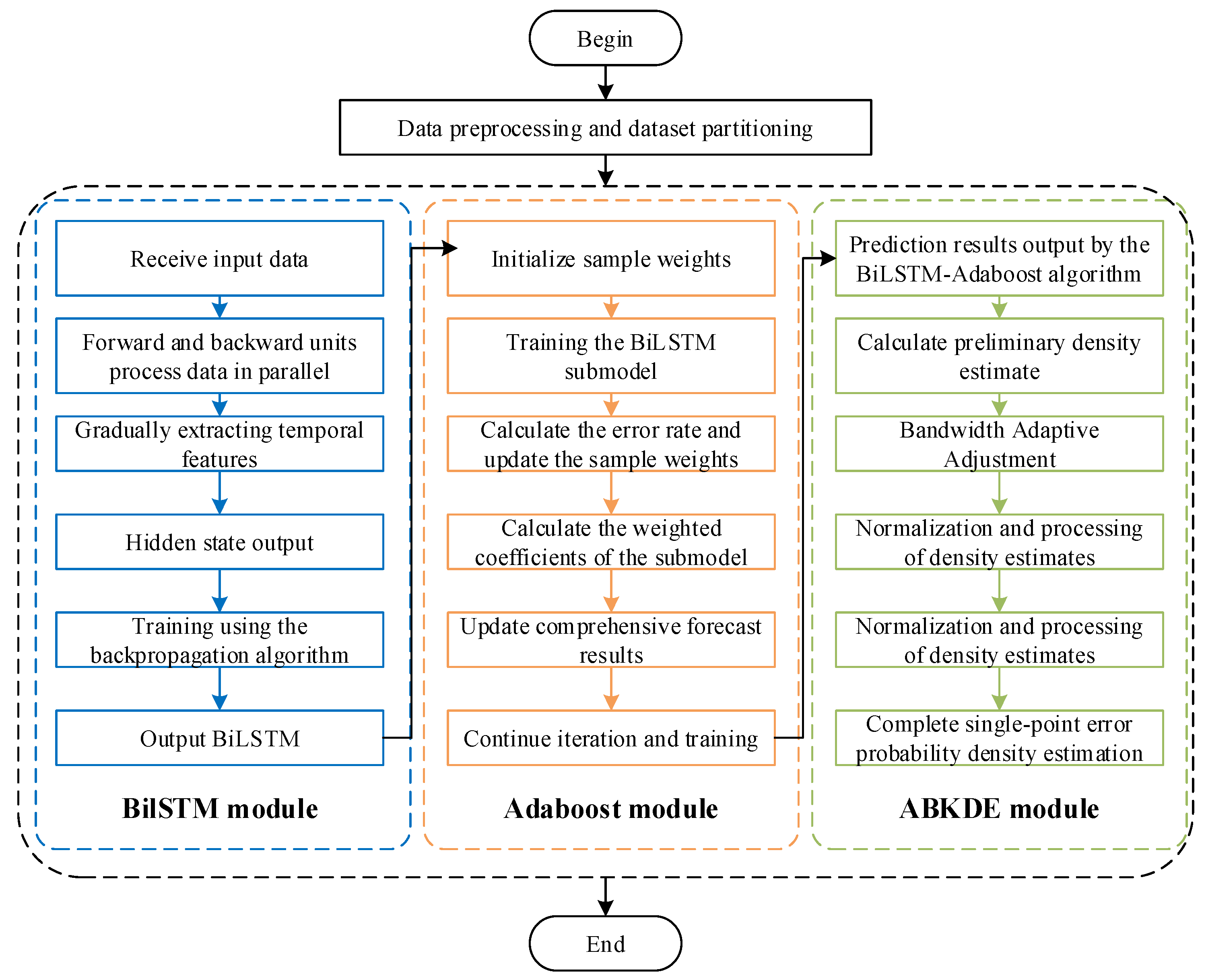
Consequently, BiLSTM addresses the challenge of modeling temporal dependencies in time series data, while Adaboost enhances model robustness and predictive accuracy. Additionally, ABKDE quantifies the uncertainty associated with the forecast results. The integration of these three components offers significant advantages, effectively compensating for the limitations of individual algorithms. The overall algorithmic workflow is illustrated in Figure 5.

Figure 5. The framework of the proposed BiLSTM-Adaboost-ABKDE algorithm for wind power forecasting.

3.5. Model Training and Validation Process

(1)

Model Architecture and Hyperparameter Settings: Each BiLSTM submodel has an input window length of L = 24 h and a prediction stride of H = 6 h.

The network comprises two BiLSTM layers: the first layer contains 64 hidden units, and the second layer contains 32 hidden units, with a single-value regression output. The Adam optimizer is employed, with an initial learning rate of 0.001 adjusted via learning rate decay. The batch size is set to 64, with 100 training epochs. Early stopping is enabled (patience = 10) to prevent overfitting. An ensemble of T = 10 BiLSTM submodels is formed, using a weighted update factor ${\alpha }_{\mathrm{t}}={\displaystyle \frac{1}{2}}\ln {\displaystyle \frac{1-{\epsilon }_t}{{\epsilon }_t}}$ per iteration, where ${\epsilon }_t$ weighted error of the current submodel. ABKDE employs a Gaussian kernel function combined with an adaptive bandwidth selection strategy. Bandwidth adjustment is based on Silverman’s empirical rule and adapts to local data density:

$$h_i=h_0·{({\displaystyle \frac{{\mathrm{p}}_{\mathrm{i}}}{\overline{p}}})}^{-\gamma },\gamma =0.5$$

(39)

where $h_0$ is the global bandwidth, ${\mathrm{p}}_{\mathrm{i}}$ is the local density estimate, and $\gamma =0.5$ is the bandwidth adjustment coefficient.

In this network, the input window length L = 24 h and the prediction horizon H = 6 h were selected based on preliminary experiments and sensitivity analysis. When L is set to 24 h, the model effectively captures the daily wind speed fluctuation patterns. The prediction horizon of H = 6 h enables the model to forecast short-term power output while maintaining a balance between training time and prediction accuracy. Sensitivity analysis indicates that although increasing the value of L allows the model to capture more historical information, the prediction accuracy gradually stabilizes within a certain range. On the other hand, smaller values of L tend to lead to overfitting.

After conducting experiments with different batch sizes, it was found that a batch size of 64 achieves a good balance between computational efficiency and training stability.

Experimental results confirmed that increasing the number of sub-models contributes to improving the robustness and stability of the model. The final choice of T = 10 sub-models, combined with AdaBoost’s weighting mechanism, significantly enhances the model’s ability to identify difficult-to-predict samples, particularly in scenarios with extreme gusts and rapid wind speed changes.

(2)

Training Process and Validation

To evaluate the model’s training effectiveness and generalization capability, experiments were conducted using training and validation sets. To evaluate the model’s performance and generalization ability, a structured data partitioning approach was employed, which divides the dataset into training, validation, and testing subsets. For the BiLSTM base learner, the same 70%/20%/10% split is used: the BiLSTM model is first trained on the 70% training subset and its hyperparameters are tuned on the 20% validation subset before being combined by the Adaboost ensemble, while the remaining 10% test subset is only used for the final performance evaluation.

The training set was used to optimize the model parameters by learning from historical data, while the validation set was utilized for hyperparameter tuning to mitigate overfitting. The testing set was reserved to assess the final predictive performance of the model on unseen data, ensuring an unbiased evaluation.

Furthermore, to enhance the robustness of the model, the validation and testing datasets were selected from different time periods, thus accounting for varying wind conditions and seasonal variations.

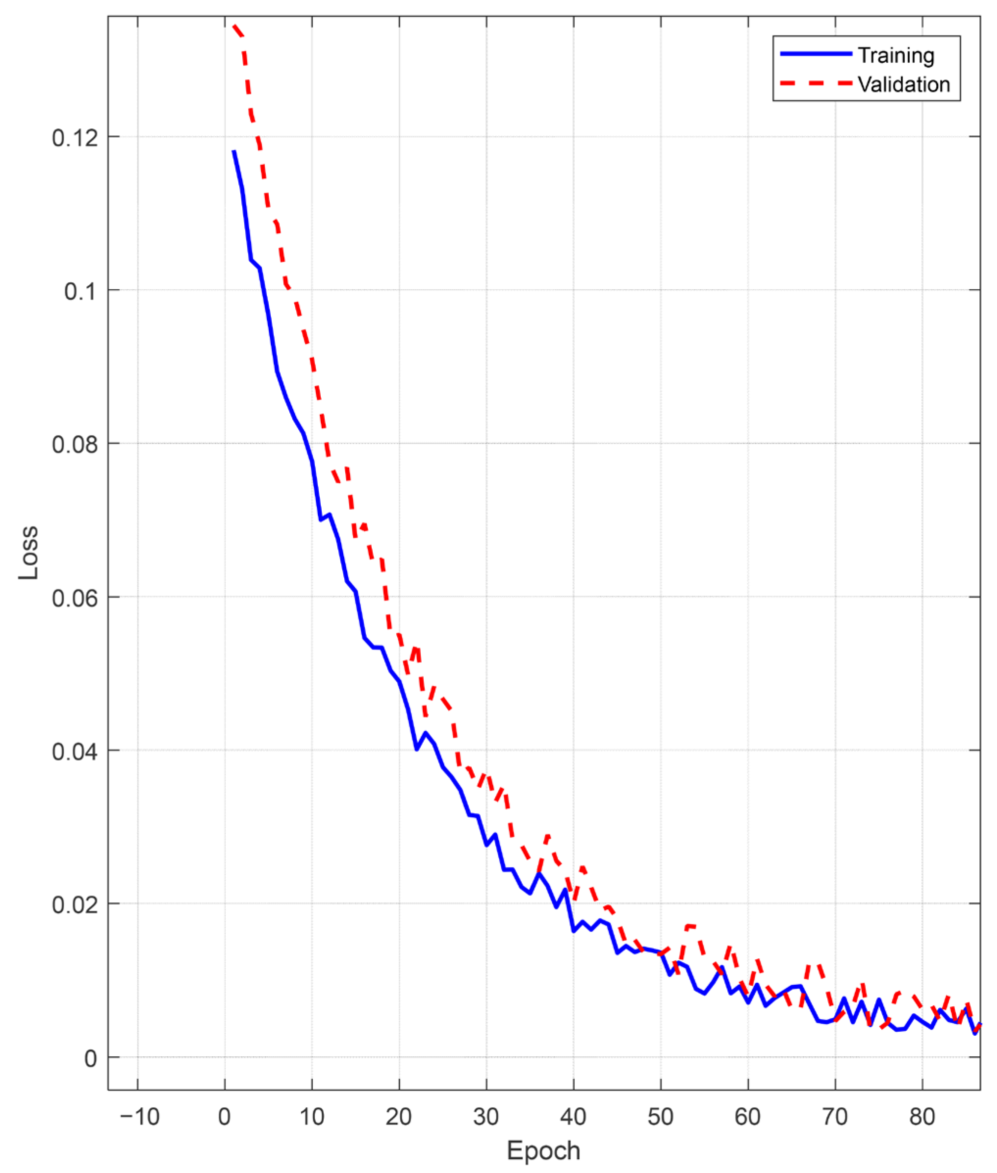
Figure 6 illustrates the performance evolution during training and validation.

Figure 6. Loss of training and validation sets over epochs.

Both training loss and validation loss stabilized after approximately 60 epochs, indicating that the model converged during training and did not exhibit overfitting.

To further evaluate the practicality of the proposed BiLSTM-Adaboost-ABKDE model, we compared its training and prediction process in terms of computation time and resource consumption with that of the standalone BiLSTM model. The experimental results are shown in Table 2.

Table 2. Comparison chart of computation time and resource consumption.

Model	Training Time (Seconds)	Prediction Time (Seconds)	GPU Utilization (%)	Average MAPE (%)
BiLSTM	305	18	72	6.15
BiLSTM-Adaboost-ABKDE	338	22	83	4.79

As shown in the table, the computational cost of the BiLSTM-Adaboost-ABKDE model is slightly higher than that of the standalone BiLSTM model, with training time and prediction time increasing by 10% and 22%, respectively (approximately 33 s and 4 s). However, despite the modest increase in computational cost, the hybrid model demonstrates a significant improvement in prediction accuracy, particularly under extreme weather conditions, showing superior stability and robustness. Especially in high-noise and small-sample wind power data environments, the BiLSTM-Adaboost-ABKDE model performs better in terms of robustness and generalization, with the average MAPE decreasing from 6.15% to 4.79%. These results suggest that, despite the increased computational cost, the hybrid model’s advantages in accuracy and stability are clear, making it a promising tool for practical wind farm risk assessment and scheduling applications.

4. Risk Assessment Indicators and Calculation Methods for Wind Farms Under Extreme Gusts

4.1. Wind Farm Risk Assessment Indicator System

To comprehensively characterize the operational risks that wind power integration may pose to the power system under extreme gust conditions, this paper builds upon traditional indicators such as voltage overlimit, power flow overlimit, load loss, and power shortage, and further introduces three key risk indicators reflecting the operational limit states of the power grid: load shedding risk ($R_{CUT}$), transmission line active power overlimit risk ($R_{LINE}$), and node voltage overlimit risk ($R_V$). These three indicators, based on the severity of system fault responses, can more accurately reflect the boundary stability and resilience of system operation. Based on this, this paper proposes using a comprehensive risk indicator as the overall risk assessment indicator for wind farm system levels.

(1)

Load shedding risk index ($R_{CUT}$): When the power grid experiences insufficient power supply, load shedding may occur. The load shedding risk index can be calculated by weighting the probability and severity of load shedding under various conditions, as expressed by the following formula:

$$R_{\mathrm{CUT}}={\displaystyle \sum _{k=1}^K{p}_W}(E_k)·p_g(E_k)·p_{\mathrm{line}}(E_k)·p_r(E_k)·S_{\mathrm{ev}\text{-}\mathrm{CUT}}(E_k)$$

(40)

Among them, $S_{\mathrm{ev}\text{-}\mathrm{CUT}}(E_k)$ is the severity of load shedding, defined as:

$$S_{\mathrm{ev}\text{-}\mathrm{CUT}}(E_k)={\displaystyle \frac{C_c(E_k)}{P_{\mathrm{load}}}}\times 100\%$$

(41)

(2)

Transmission line active power limit risk indicator ($R_{\mathrm{LINE}}$): If the operating power of the transmission line exceeds the safety limit under certain conditions, it may cause line overload or even tripping. The risk indicators are as follows:

$$R_{\mathrm{LINE}}={\displaystyle \sum _{k=1}^K{p}_W}(E_k)·p_g(E_k)·p_{\mathrm{line}}(E_k)·p_r(E_k)·S_{\mathrm{ev}\text{-}\mathrm{LINE}}(E_k)$$

(42)

Among them:

$$S_{\mathrm{ev}\text{-}\mathrm{LINE}}(E_k)={\displaystyle \sum _{m=1}^M\frac{\max (p_m(n)-p_{m,\max }(m),0)}{e-1}}$$

(43)

(3)

Node voltage limit risk indicator ($R_V$): If the node voltage exceeds the set upper or lower limit, it will affect power quality and even trigger protection mechanisms. The risk indicator is defined as follows:

$$R_V={\displaystyle \sum _{k=1}^K{p}_W}(E_k)·p_g(E_k)·p_{\mathrm{line}}(E_k)·p_r(E_k)·S_{e\text{-}\mathrm{V}}(E_k)$$

(44)

Among them, the severity function is:

$$S_{\mathrm{ev}\text{-}\mathrm{V}}(E_k)={\displaystyle \sum _{i=1}^N\frac{e^{\max (0.9-U_i,U_i-1.0)}-1}{e-1}}$$

(45)

(4)

Comprehensive risk indicator ($R_{\mathrm{CR}}$): The final comprehensive risk indicator is calculated by weighting and combining the three types of risk mentioned above:

$$R_{\mathrm{CR}}={\omega }_1·R_{\mathrm{CUT}}+{\omega }_2·R_{\mathrm{LINE}}+{\omega }_3·R_V$$

(46)

Among them, ${\omega }_1$, ${\omega }_2$ and ${\omega }_3$ are the weighting coefficients for each risk indicator.

In order to link the three risk indices to physical and operational constraints, the following settings are adopted in this study. For the load shedding risk index $R_{CUT}$, the severity at each time step is defined as the ratio between the involuntary load shedding and the total system load at that time. Accordingly, $R_{CUT}$ is a dimensionless index with values between 0 and 1, and $R_{CUT}$ = 0 corresponds to secure operation without any load shedding. For the transmission line active power limit risk index $R_{LINE}$, the power flow limit of each branch is set equal to its rated active power $P_{ij,\max }$ as given in the IEEE RTS-79 dataset. $R_{LINE}$ remains zero as long as the absolute value of the active power flow of a branch does not exceed its limit P_ij,max, and starts to increase when this thermal limit is approached or violated. For the node voltage limit risk index $R_V$, the admissible per-unit voltage range [$V_{\min }$, $V_{\max }$] is taken as 0.9–1.1 p.u. for all buses, corresponding to the typical ±10% band around the nominal voltage used in transmission-system security analysis.

4.2. Risk Assessment Calculation Method

The BiLSTM-Adaboost-ABKDE model outputs two key dimensions of information: first, point forecasts of wind power output representing the most probable power output under given input conditions; second, the probability density distribution of power values, quantified by ABKDE (Adaptive Bandwidth Kernel Density Estimation) to capture prediction uncertainty. These outputs are coupled with the grid’s real-time operational status through Integrated Trend Analysis (ITA) and Time Series Probability Weighting (TPW) methods, respectively, to calculate various risk metrics.

4.2.1. Predictive Data Preprocessing and Grid Operation Status Simulation

When establishing a risk assessment system for wind farms under extreme gust conditions, the primary task is to effectively convert the predictive outputs of the BiLSTM-Adaboost-ABKDE model into input data suitable for grid analysis.

During the data preprocessing stage, we perform temporal alignment and spatial allocation on the wind power forecast values generated by the model. On the temporal dimension, the 6 h point forecast sequence ${\{\stackrel{\wedge }{p_{w}f(t)}\}}_{t=1}^6$ with 1 h intervals and its corresponding probability density function ${\{f({\stackrel{\wedge }{p}}_w(t))\}}_{t=1}^6$ require interpolation to convert them into 15 min interval data matching the grid simulation step size.

Spatially, the total forecasted wind power is distributed to three wind farm interconnection nodes (BUS7, BUS14, and BUS18) according to a preset ratio, consistent with the network structure of the IEEE RTS-79 system. In this system, BUS7, BUS14, and BUS18 are representative load buses located in different areas of the network and connected to multiple transmission corridors, and are therefore adopted in this study as equivalent interconnection points for the aggregated wind farm, reflecting typical transmission-level locations where large-scale wind power would be integrated.

For grid modeling, we employ an improved random power flow calculation method to inject the processed forecast data into system analysis. Unlike traditional deterministic power flow, this method addresses forecast uncertainty through Monte Carlo simulation. The specific process is as follows: First, based on the probability density functions provided by ABKDE, 1000 equally probable wind power scenarios are generated for each time slice. Then, for each scenario, the following power balance equation is solved:

$$g(x)=p_{wind}+p_{gen}-p_{load}-p_{loss}(x)=0$$

(47)

where $\mathrm{x}={\left[\mathrm{V},\mathsf{\theta }\right]}^{\mathrm{T}}$ represents the system state variables, including node voltage magnitudes and phase angles. Through large-scale scenario calculations, we obtain probability distributions for state variables such as node voltages and line powers, providing a statistical foundation for risk assessment.

4.2.2. Convergence Trend Analysis Method

The core of the Convergence Trend Analysis (ITA) method [29] lies in utilizing point prediction results provided by the BiLSTM-Adaboost-ABKDE model, combined with historical operational data, to identify and quantify the dynamic evolution trends of system risk indicators under the influence of extreme gusts. This approach does not simply substitute predicted values into static formulas but instead constructs a time-varying probability distribution that integrates historical patterns with current predictive information, thereby achieving forward-looking perception of risk trends.

Specifically, for line power overlimit risk, the ITA method first constructs a time-varying probability density function $f_{ITA}^l(P,t)$. This is achieved by applying sliding window kernel density estimation (KDE) to the historical power data $[P_l(t-L),P_l(t-L+1),\dots ,P_l(t-1)]$ of line l and the point prediction sequence $[{\stackrel{\wedge }{P}}_l(t),{\stackrel{\wedge }{P}}_l(t+1),\dots ,{\stackrel{\wedge }{P}}_l(t+H)]$ for the future forecast period.

For illustration, the formulation of the branch power overlimit indicator in ITA is given in Equation (48):

$$R_{\mathrm{lfA}}=\left\{\begin{array}{ll}0,\hfill & P_l\le P_l^{\max }\hfill \\ {\displaystyle {\int }_{P_l^{-}}^{P_l}(P_l-P_l^{\max })}f(P_l)\mathrm{d}{P}_l,\hfill & P_l>P_l^{\max }\hfill \end{array}\right.$$

(48)

In the formula: $R_{\mathrm{lfA}}$ is the branch power limit indicator calculated by the ITA method; $f(P_l)$ is the probability distribution value obtained by fitting the historical data and predicted values of the power of the lth branch; $P_l$ is the power value; $P_l^{\max }$ is the maximum power of branch l.

4.2.3. Time-Series Probability Weighting Method

The Time-Probability Weighted Method (TPW) is a risk assessment approach based on probabilistic forecast results [30]. Its core concept is to fully leverage the comprehensive probabilistic forecast information provided by the ABKDE module, expanding risk assessment from a single “most probable scenario” to a “probability-weighted average of all possible scenarios.” This directly incorporates forecast uncertainty into the risk measurement framework.

Specifically, at each prediction time point t, ABKDE provides the probability density function $f(P_{wf}(t))$ for wind power output at that moment. Through Monte Carlo simulation, we generate numerous wind power scenarios ${\{P_{wf}^{(s)}(t)\}}_{s=1}^N$ that follow this distribution. For each scenario s, deterministic power flow calculations are performed to obtain the risk indicator value $R_{flow}^{(s),l}(t)$ for that system state. Subsequently, the comprehensive risk at time t is characterized by calculating the arithmetic mean of the risk indicators across all scenarios at that time slice. Similarly, taking the power overlimit indicator of a branch in the system as an example, as shown in the equation:

$$r_{lt}=\left\{\begin{array}{ll}0,\hfill & P_l\le P_l^{\max }\hfill \\ {\displaystyle {\int }_{P_l^{\max }}^{P_l}(P_l-P_l^{\max })}f(P_l)d{P}_l,\hfill & P_l>P_l^{\max }\hfill \end{array}\right.$$

(49)

$$R_{TPW}={\displaystyle \sum _{t=1}^{\mathrm{n}}{r}_k*(1-\frac{t-1}{T})}$$

(50)

In the formula: $r_{lt}$ represents the branch power overlimit risk assessment index for branch l at time t; T denotes the total number of prediction time points; $R_{TPW}$ indicates the branch power overlimit index for this branch calculated using the TPW method.

In practical implementation, the predictive probability distribution of wind farm power obtained from ABKDE is first used to generate a set of wind power scenarios, then the random power flow model is run for each scenario to compute the corresponding values of branch power, bus voltage and load shedding, and finally the TPW method aggregates these scenario-wise risk values into the time-varying risk indices, so that the forecast uncertainty quantified by ABKDE is directly propagated to $R_{CUT}$, $R_{LINE}$ and $R_V$.

4.3. Weighted Algorithm for Wind Farm Risk Assessment Indicators

To enhance the accuracy of wind farm risk assessment under extreme gust conditions, this study proposes an evaluation framework based on dynamic weighted fusion. By deeply integrating the Integrated Trend Analysis (ITA) and Time Series Probability Weighting (TPW) methods, it fuses three risk indicators—load curtailment risk, line power overlimit risk, and node voltage overlimit risk—into a unified system-level risk metric.

4.3.1. Risk Indicator Calculation Method Based on Model Output

At the risk indicator calculation level, this study strictly adheres to the risk assessment indicator system defined in Section 4.1, deeply coupling the wind power prediction values output by the BiLSTM-Adaboost-ABKDE model with the grid operational state. Specifically, the model-predicted wind power sequences (including point estimates and probability distributions) serve as inputs. Through time-series power flow calculations using an enhanced IEEE RTS-79 system, the dynamic operational state of the system is obtained, and various risk indicators are calculated based on this state.

4.3.2. Theoretical Basis and Implementation of ITA and TPW Weighted Fusion

The ITA method extracts the evolutionary trend of system risk by constructing a joint probability distribution between historical data and forecast results. The specific implementation includes: selecting historical operational data from the most recent 24 time-slices, combining it with power forecasts for the next 6 h, and employing adaptive bandwidth kernel density estimation to construct a time-varying probability density function. The TPW method focuses on handling instantaneous risk fluctuations caused by forecast uncertainty. Its technical approach involves: generating 1000 equally probable scenarios based on the probability distribution output from ABKDE, performing deterministic power flow calculations for each scenario, and aggregating the expected risk values at each time step using a time-decay weighting function. The time weighting function adopts an exponential decay form:

$$\varpi (t)={\displaystyle \frac{e^{-\mathsf{\lambda }(t-1)}}{{\displaystyle {\sum }_{t=1}^H{e}^{-\mathsf{\lambda }(t-1)}}}}$$

(51)

The attenuation coefficient $\mathsf{\lambda }=0.4$ was determined through optimization using historical data.

During the weighted fusion process, due to differences in data scale and distribution characteristics between the two methods, the prediction results are first normalized:

$$R_{\mathrm{ITA},\mathrm{norm}}(i)={\displaystyle \frac{R_{\mathrm{ITA}}(i)}{\max (R_{\mathrm{ITA}})}}$$

(52)

$$R_{\mathrm{TPW},\mathrm{norm}}(i)={\displaystyle \frac{R_{\mathrm{TPW}}(i)}{\max (R_{\mathrm{TPW}})}}$$

(53)

Based on the normalized results, weight coefficients are calculated through a dynamic weight allocation mechanism:

$$S_{\mathrm{ITA}}={\displaystyle \frac{{\displaystyle \sum R_{\mathrm{ITA},\mathrm{norm}}}}{{\displaystyle \sum R_{\mathrm{ITA},\mathrm{norm}}}+{\displaystyle \sum R_{\mathrm{TPW},\mathrm{norm}}}}}$$

(54)

$$S_{\mathrm{TPW}}={\displaystyle \frac{{\displaystyle \sum R_{\mathrm{TPW},\mathrm{norm}}}}{{\displaystyle \sum R_{\mathrm{ITA},\mathrm{norm}}}+{\displaystyle \sum R_{\mathrm{TPW},\mathrm{norm}}}}}$$

(55)

In the formula, $S_{\mathrm{ITA}}$ and $S_{\mathrm{TPW}}$ are the weighting coefficients for the ITA and TPW methods, respectively. Based on the above coefficients, the integrated single risk indicator can be calculated as follows:

$$R_i^{\mathrm{fused}}=S_{\mathrm{ITA}}·R_{\mathrm{ITA},\mathrm{norm}}(i)+S_{\mathrm{TPW}}·R_{\mathrm{TPW},\mathrm{norm}}(i)$$

(56)

Finally, to construct a system-level comprehensive risk indicator, the Weighted Sum Method (WSM) is employed to synthesize the various fused individual risk indicators, defined as follows:

$$R_{CR}={\varpi }_1·R_{CUT}^{\mathrm{fused}}+{\varpi }_2·R_{LINE}^{\mathrm{fused}}+\varpi 3·R_V^{\mathrm{fused}}$$

(57)

In the formula, ${\varpi }_1$, ${\varpi }_2$ and ${\varpi }_3$ represent the weighting coefficients for each category of risk indicators.

In order to examine the robustness of the comprehensive risk indicator with respect to these weighting coefficients, a simple sensitivity check was carried out in the case study: the weights were perturbed within a reasonable range while being renormalized to sum to one, and the resulting $R_{CR}$ time series showed changes in absolute magnitude but preserved the main temporal patterns and the relative ordering of risk levels across operating conditions, indicating that the qualitative conclusions drawn from CRR are not overly sensitive to moderate variations in the weights.

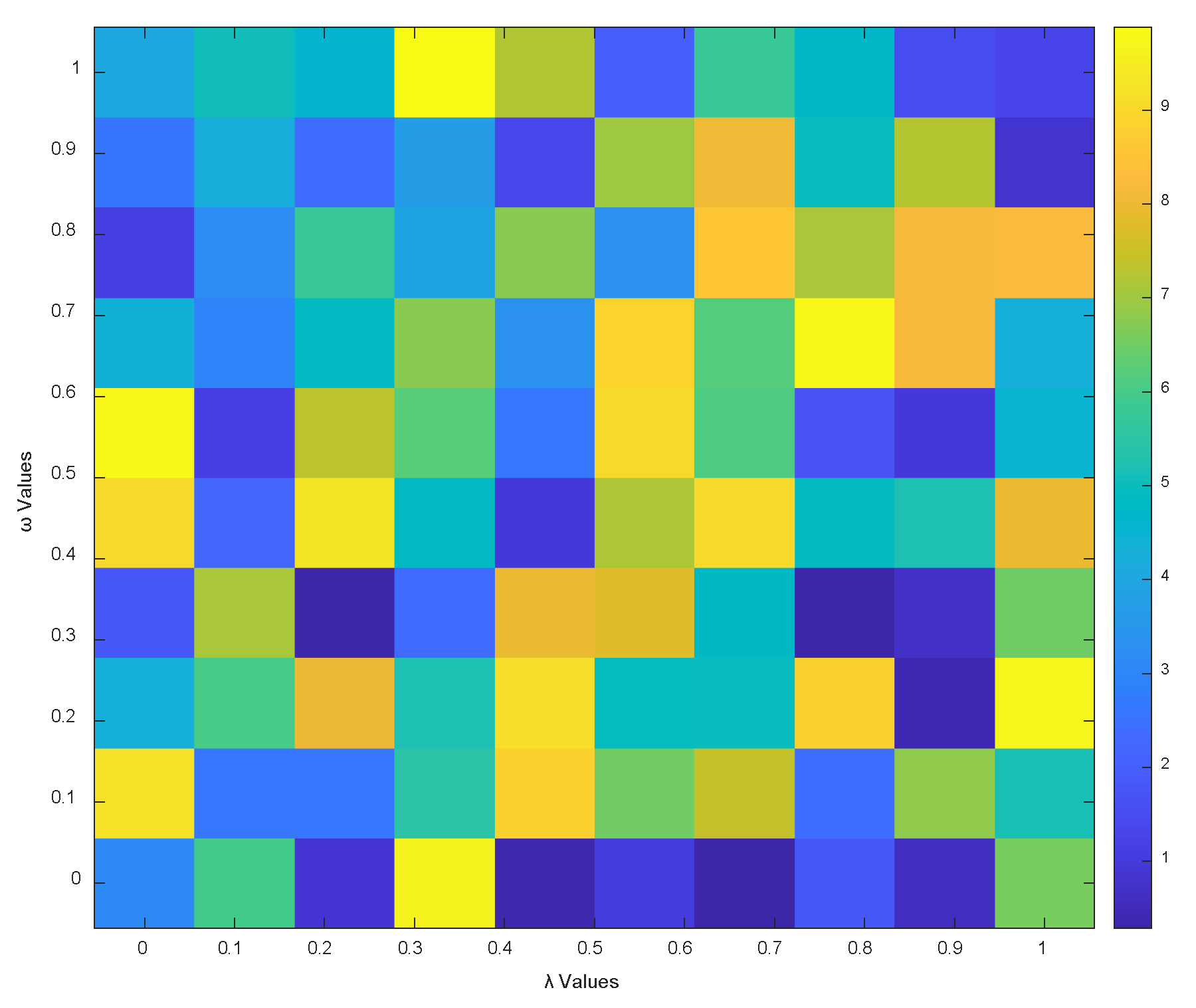
Considering the impact of λ and ω on the final risk assessment results, we employed a Bayesian optimization approach to improve the accuracy and stability of the model. The core idea is as follows: In the experiments, λ and ω were searched within the range [0, 1]. Then, the Bayesian optimization algorithm was used to minimize the MAPE (Mean Absolute Percentage Error), with the goal of finding the optimal parameter combination. During the optimization process, cross-validation was introduced to ensure that the optimized values of λ and ω had good generalization ability. We divided the dataset into a training set (70%), a validation set (20%), and a test set (10%), and applied K-fold cross-validation during the training process, calculating the MAPE for each fold to ensure consistency in the MAPE results across different folds.

Figure 7 shows the impact of different combinations of λ and ω on the MAPE. Through Bayesian optimization, we found that when λ = 0.4 and ω = 0.3, the model achieved the lowest MAPE, thus validating the effectiveness of the optimization process.

Figure 7. Impact of λ and ω on MAPE.

4.4. Wind Farm Risk Assessment Process

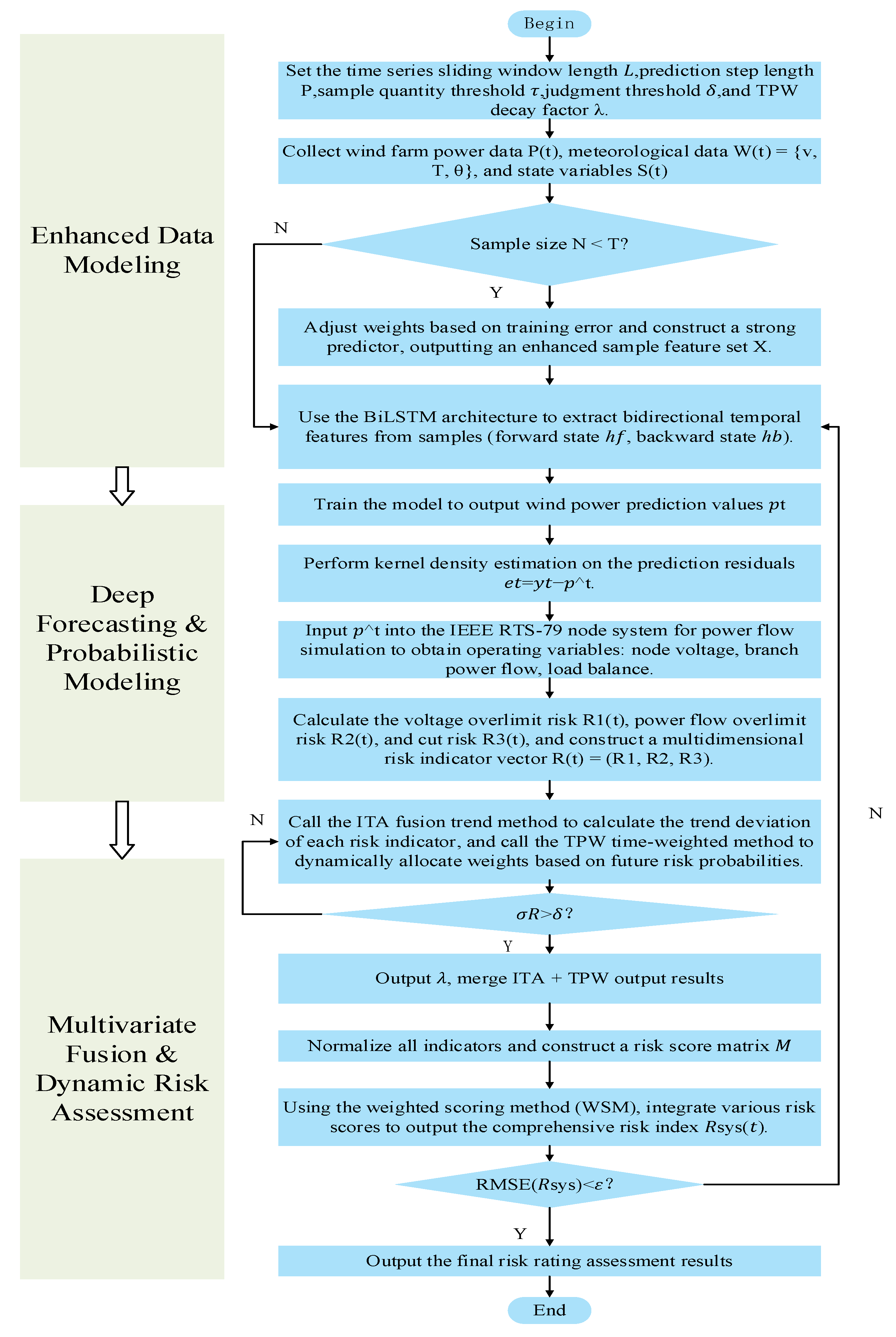
The wind farm operation risk assessment process developed in this study is shown in Figure 8. The overall process consists of three stages: power prediction under extreme gust disturbance conditions, probabilistic modeling, and multi-dimensional risk indicator assessment. The specific steps are as follows:

Figure 8. Research flowchart of the wind farm operational risk assessment method under extreme gust conditions.

(1)

Data initialization and sample construction: Historical meteorological data (wind speed, wind direction, temperature) and operational data (wind power) from the wind farm are collected and subjected to normalized standard processing. A sliding window is used to construct the time series input sample set $X\in R^{T\times d}$, which is utilized for subsequent model training.

(2)

BiLSTM-Adaboost modeling and prediction enhancement: BiLSTM captures the bidirectional time-dependent characteristics of wind power data and constructs multiple submodels. Adaboost dynamically adjusts the weights of the submodels to enhance adaptability to small samples and extreme disturbances, ultimately outputting the wind power prediction value ${\widehat{P}}_{\mathrm{t}}$

(3)

ABKDE probability modeling: Based on the point prediction values output by BiLSTM-Adaboost, kernel density estimation is performed on the residuals to calculate the confidence interval $\left[{\widehat{P}}_t^{\mathrm{low}},{\widehat{P}}_t^{\mathrm{up}}\right]$ and probability density distribution $\mathrm{f}({\widehat{P}}_{\mathrm{t}})$ of the predicted power, thereby quantifying the uncertainty of the prediction.

(4)

System state variable assessment: Predictive power is input into the IEEE RTS-79 node system for power flow simulation to obtain key operating state variables, including node voltage $U_i$, branch power flow $P_{ij}$, load balance $L_i$, etc.

(5)

Multi-dimensional risk indicator calculation: Based on system state variables, a risk assessment indicator system is constructed, including:

$$\mathrm{Voltage} \mathrm{limit} \mathrm{risk}: R_{\mathrm{vol}}={\displaystyle \frac{N_{\mathrm{out}}^U}{N_{\mathrm{total}}^U}}$$

$$\mathrm{Power} \mathrm{flow} \mathrm{limit} \mathrm{risk}: R_{\mathrm{flow}}={\displaystyle \frac{N_{\mathrm{out}}^P}{N_{\mathrm{total}}^P}}$$

$$\mathrm{Load} \mathrm{shedding} \mathrm{risk}: R_{\mathrm{load}}={\displaystyle \frac{L_{\mathrm{unserved}}}{L_{\mathrm{total}}}}$$

(6)

Risk Indicator Trend Assessment (ITA): Analyze the current trends of various risk indicators and their historical means and variances, calculate trend deviation degrees $\Delta R_{\mathrm{vol}}$, $\Delta R_{\mathrm{flow}}$, and $\Delta R_{\mathrm{load}}$, and quantify the degree of deviation in indicator stability.

(7)

Time-weighted risk indicator (TPW): Based on the risk probability at each time step in the prediction interval, set a decreasing weight function $w_t={\mathrm{e}}^{-\mathsf{\lambda }(T-t)}$ and calculate the weighted risk score: $R_{\mathrm{tpw}}={\displaystyle \sum w_t}\cdot R_t$.

(8)

Fusion processing and weighted output: The ITA results and TPW results are normalized and fused to obtain a comprehensive risk score vector:

$$R_{\mathrm{final}}=\alpha ·R_{\mathrm{ita}}+(1-\alpha )·R_{\mathrm{tpw}}$$

(9)

Risk status assessment and feedback mechanism: Assess the integrated risk score results. If the score exceeds the set threshold, trigger a “high risk” alert; otherwise, update the historical sequence of status indicators and enter the next assessment cycle.

5. Experimental Results and Analysis

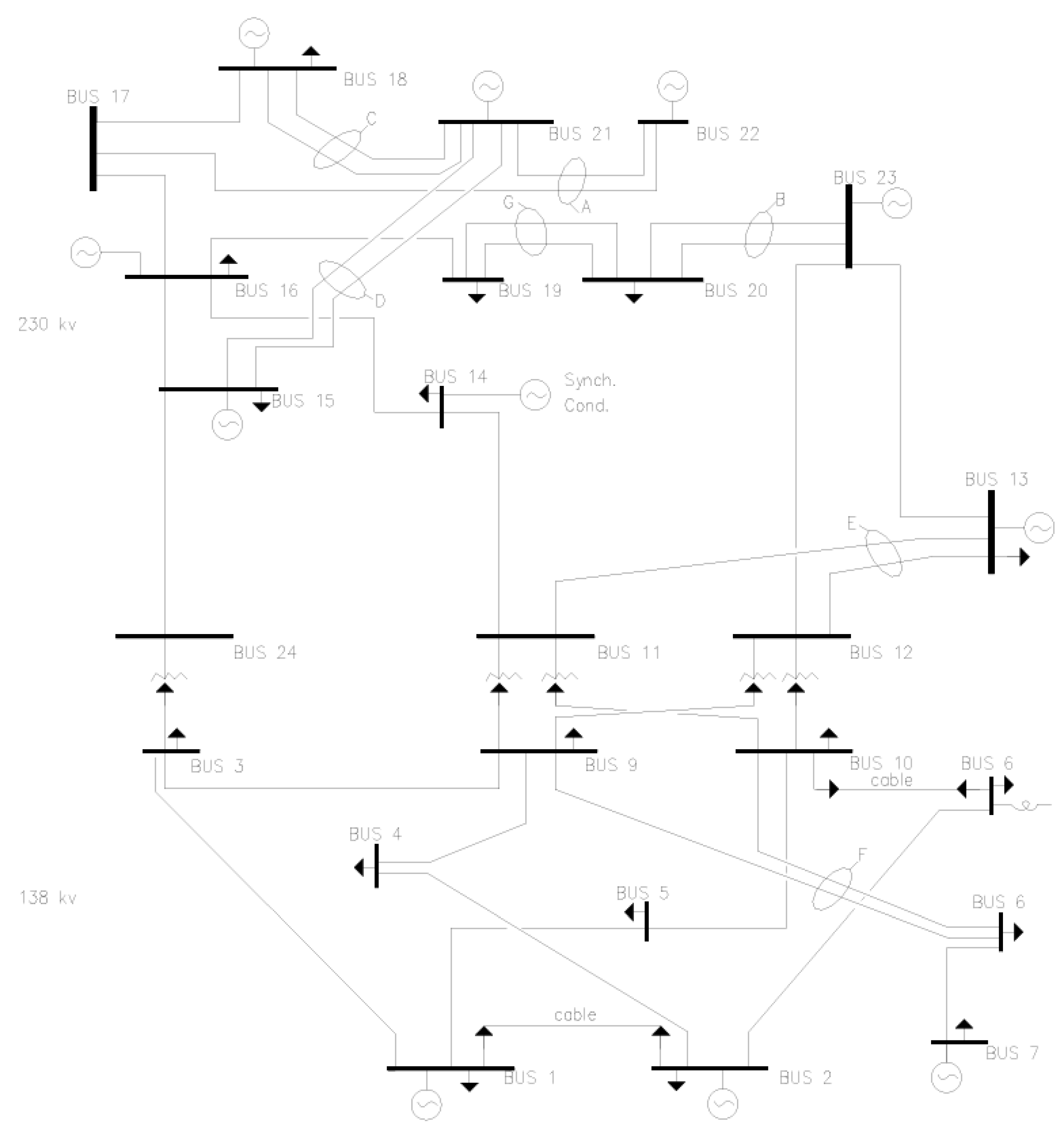
This study uses the IEEE RTS-79 power system as the test case for validation (Figure 8). Widely employed in studies on dispatch optimization, power flow analysis, and operational risk assessment, the RTS-79 system consists of 24 load buses, 38 transmission lines, and 32 generators, with voltage levels organized into two tiers: 230 kV and 138 kV (Figure 9).

Figure 9. Flow chart of coordinated control of PV-based energy storage and black start.

To simulate renewable energy integration, wind farms are placed at buses 7 (300 MW), 14 (150 MW), and 18 (80 MW). Their output profiles are generated from real wind speed data, enabling the modeling of dynamic disturbance effects of wind power in a typical grid environment.

5.1. Dataset Description and Preprocessing

The dataset used in this paper originates from a wind farm in Hebei Province, China. Data collection spanned from 1 March 2020, to 31 May 2023, with a sampling interval of one hour, yielding approximately 3500 data records. The dataset was divided into training, validation, and test sets in a 7:2:1 ratio to ensure temporal continuity and prevent forward information leakage. Data was collected in real-time via the wind farm’s SCADA (Supervisory Control and Data Acquisition) system, encompassing typical meteorological conditions in the region, such as springtime severe convective weather and winter temperature inversions.

The experimental environment configuration is as follows: Operating system: Windows 11; CPU: Intel^® Core™ i7-14650HX 2.20 GHz; GPU: NVIDIA GeForce RTX 4050; Python version: 3.9.21; TensorFlow version: 2.10.0; CUDA version: 11.2.

To enhance data diversity and validate model robustness, this study incorporates the wind energy dataset provided by NREL (National Renewable Energy Laboratory). This dataset contains high-frequency wind speed and energy data from 2019 to 2020, resampled to match the 1 h resolution of the primary dataset. Cross-validation ensures the model’s adaptability and robustness under varying wind resource conditions.

5.2. Wind Power Forecasting Results

To evaluate the effectiveness of the proposed BiLSTM-Adaboost-ABKDE algorithm, this study conducted hourly wind power forecasting experiments using actual wind speed and power output data over a specific timeframe. The data originated from a typical wind farm in Hebei Province, utilizing 100 consecutive hours of historical data from spring (a season characterized by frequent gusts). The data featured a 1 h temporal resolution and primarily focused on the active power output of the wind farm connected to nodes 7, 14, and 18. Considering the impact of extreme gusts on power fluctuations, this study specifically selected periods with more intense wind speed variations for experimentation.

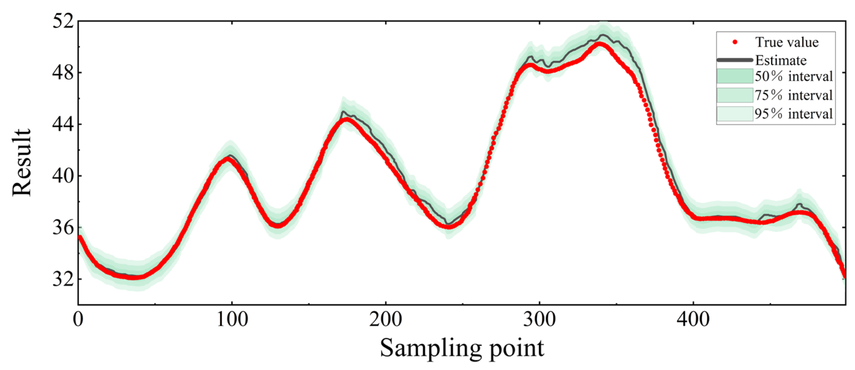
Figure 10 first presents the forecasting results and predictive uncertainty of the proposed model on this representative test segment. The horizontal axis denotes the sampling index and the vertical axis denotes the corresponding normalized wind power output. In Figure 8, the red markers represent the measured values, the black solid line represents the predictive mean of the model, and the shaded regions from dark to light correspond to the 50%, 75% and 95% prediction intervals derived from the ABKDE-estimated predictive distribution at each sampling point. Most observations fall within the 95% band and the majority lie inside the 75% band, indicating that the prediction intervals are reasonably calibrated.

Figure 10. Wind power forecasts with prediction intervals.

Furthermore, to validate the performance of the proposed model, the following representative models were selected as baselines for comparative experiments:

GRU (Gated Recurrent Unit): A lightweight recurrent neural network architecture capable of capturing short-term dependencies, but prone to convergence instability when handling highly volatile samples.

Transformer: An attention-based model suitable for long-sequence modeling, but prone to overfitting in small-sample scenarios.

GAN-based model (Generative Adversarial Network-based time series prediction): Primarily used for data augmentation and uncertainty modeling, but susceptible to noise interference that degrades model performance.

BiLSTM-Adaboost (without ABKDE): A combination of bidirectional temporal learning and ensemble weighted prediction, used to validate the contribution of the ABKDE algorithm in uncertainty modeling.

In comparative experiments, all models employed identical input features, sample partitioning, and hyperparameter search strategies. Predictive performance was quantified using RMSE (Root Mean Square Error) and MAPE (Mean Absolute Percentage Error) metrics to comprehensively evaluate different models’ capabilities in wind power forecasting.

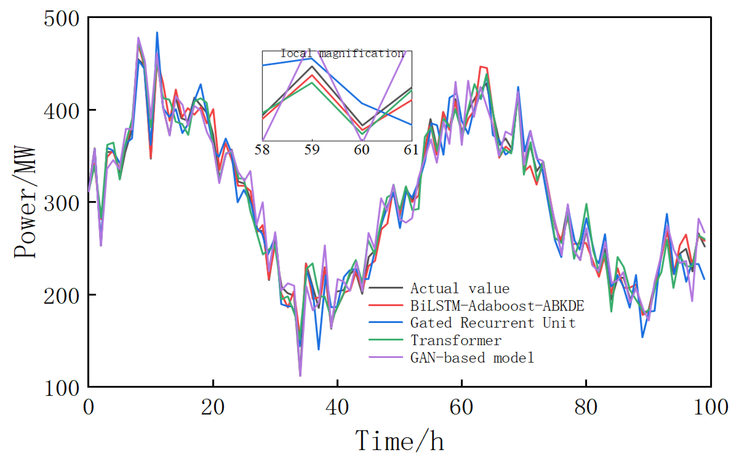
Figure 11 further compares the proposed BiLSTM–Adaboost–ABKDE algorithm with Gated Recurrent Unit (GRU), Transformer and GAN-based models in terms of hourly prediction accuracy and dynamic response performance across a representative 100 h interval. Overall, all models effectively tracked the general fluctuation trends of wind power output. However, significant differences emerged in handling local abrupt changes, such as the rapid wind power increase observed between hours 58 and 61.

Figure 11. Multi-model prediction comparison chart.

Particularly during the rapid wind power increase phase, while the GRU model smoothly tracked power changes, its inherent strong short-term dependencies caused prediction curves to lag when confronting sudden wind speed shifts, failing to capture abrupt features in a timely manner. The Transformer model, while suitable for long-sequence modeling and capable of capturing long-term dependencies through its attention mechanism, is prone to overfitting in small-sample scenarios. This compromises prediction accuracy, leading to substantial errors during specific time periods. The GAN-based model, though effective at enhancing data diversity and modeling uncertainty, suffers from unstable oscillations in its predictions due to susceptibility to noise interference, particularly under extreme wind speed fluctuations.

In contrast, the proposed BiLSTM-Adaboost-ABKDE model rapidly responds to sudden wind speed changes while maintaining smooth and accurate prediction trajectories across the dynamic range of wind power output. This model employs Bidirectional Long Short-Term Memory (BiLSTM) to capture nonlinear dynamic variations in wind power output. Combined with the AdaBoost weighting mechanism, it enhances adaptability to hard-to-predict samples. Utilizing the ABKDE algorithm for quantifying prediction uncertainty modeling, it effectively reduces noise interference, demonstrating superior generalization performance and convergence stability under conditions of small sample size and high data volatility.

5.2.1. Predictive Performance Evaluation Metrics

In the preceding section, the fitting performance of each model during typical periods was evaluated using point predictions. To quantitatively assess prediction accuracy and interval reliability, a standard set of error metrics is employed: Mean Absolute Percentage Error (MAPE), Root Mean Square Error (RMSE), Prediction Interval Coverage Probability (PICP), and Prediction Interval Normalized Average Width (PINAW). These metrics enable a detailed interval-based comparison of the models, thereby validating the accuracy and practical applicability of the proposed method. The definitions are as follows:

$$\mathrm{MAPE}={\displaystyle \frac{1}{n}}{\displaystyle \sum _{t=1}^n\left|\frac{y_t-{\widehat{y}}_t}{y_t}\right|}\times 100\%$$

(58)

$$\mathrm{RMSE}=\sqrt{{\displaystyle \frac{1}{n}}{\displaystyle \sum _{t=1}^n{(y_t-{\widehat{y}}_t)}^2}}$$

(59)

$$\mathrm{PICP}={\displaystyle \frac{1}{n}}{\displaystyle \sum _{t=1}^n\mathbb{I}}\left(y_t\in [{\widehat{y}}_t^L,{\widehat{y}}_t^U]\right)$$

(60)

$$\mathrm{PINAW}={\displaystyle \frac{1}{nR}}{\displaystyle \sum _{t=1}^n\left({\widehat{y}}_t^U-{\widehat{y}}_t^L\right)}$$

(61)

Among them, $y_t$ is the actual value, ${\widehat{y}}_t$ is the predicted value, ${\widehat{y}}_t^L$ and ${\widehat{y}}_t^U$ are the lower and upper confidence limits of the prediction, respectively, R is the data value range, and $\mathbb{I}\left(·\right)$ is the indicator function.

Table 3 summarizes the performance comparison of the proposed BiLSTM–Adaboost–ABKDE model with three baseline models (GRU, Transformer, and GAN-based model) under different confidence levels (50%, 75%, and 95%). The evaluation metrics include MAPE (Mean Absolute Percentage Error), RMSE (Root Mean Square Error), PICP (Prediction Interval Coverage Probability), and PINAW (Prediction Interval Normalized Average Width), which comprehensively reflect both point prediction accuracy and interval prediction reliability. Definitions of these metrics are provided in Table 1.

Table 3. Prediction Performance Evaluation Metrics.

Confidence Level	Algorithm in This Paper				Gated Recurrent Unit				Transformer				GAN-Based Model
	MAPE	RMSE	PICP	PINAW	MAPE	RMSE	PICP	PINAW	MAPE	RMSE	PICP	PINAW	MAPE	RMSE	PICP	PINAW
95.0	4.32	7.11	96.4	7.59	6.85	10.34	91.2	10.84	6.13	9.22	92.4	9.41	5.79	8.02	92.2	15.35
75.0	4.96	6.45	81.3	5.04	7.42	9.75	72.6	7.32	6.92	8.51	76.0	6.80	6.43	7.45	78.6	10.57
50.0	5.84	5.82	57.3	3.44	8.13	9.11	46.8	5.16	7.85	7.90	50.2	4.42	7.26	6.91	49.2	4.90

Specifically, at the 95% confidence level, the model achieves an RMSE of 7.11, reducing the error by 31.2% compared to GRU (10.34), 22.9% compared to Transformer (9.22), and 11.3% compared to GAN-based model (8.02). The MAPE also drops to 4.32%, which is 36.9% lower than GRU and 29.5% lower than Transformer. This trend holds at both 75% and 50% confidence levels, showing that the proposed model maintains stable prediction accuracy under various uncertainty levels.

Regarding interval prediction, the proposed model achieves the highest PICP (96.36%), indicating better coverage of true wind power values in the prediction intervals, and the smallest PINAW (7.59%), suggesting narrower and more reliable prediction intervals compared to other models. This means that the proposed model strikes a good balance between high coverage and minimal uncertainty in its predictions.

In extreme gust conditions, the BiLSTM–Adaboost–ABKDE model shows less fluctuation in prediction errors, indicating lower variance and better robustness against noise compared to other models. This is attributed to the synergy of BiLSTM capturing the temporal dependencies, Adaboost enhancing model robustness through ensemble learning, and ABKDE effectively modeling the uncertainty of prediction errors.

Furthermore, the model exhibits better performance with fewer data and high volatility, confirming its strong generalization ability in small-sample and high-uncertainty scenarios. The GAN-based model, while capable of generating strong predictions in some cases, suffers from instability and poor convergence under extreme gusts due to its reliance on data distribution learning.

5.2.2. Paired t-Test

To further validate the performance improvement of the proposed BiLSTM-Adaboost-ABKDE model in wind power forecasting, we conducted a paired t-test to determine if the improvements were statistically significant. The paired t-test is a statistical method used to compare the mean differences between two related samples. In this study, we used the paired t-test to compare the prediction performance of the BiLSTM-Adaboost-ABKDE model with that of the GRU, Transformer, and GAN models.

The paired t-test calculates the mean and standard deviation of the differences between the two sets of samples to obtain the t-value. Then, based on the t-value, the p-value is computed, which is used to assess the statistical significance of the difference between the models.

$$\mathrm{t}={\displaystyle \frac{\overline{d}}{\raisebox{1ex}{$s_d$}\!\left/ \!\raisebox{-1ex}{$\sqrt{n}$}\right.}}$$

(62)

where $\overline{\mathrm{d}}$ represents the mean of the differences between the two sets of samples, $s_d$ represents the standard deviation of the differences, and n denotes the number of samples.

For the GRU, Transformer, and GAN models, the p-values from the paired t-test are 0.03, 0.04, and 0.02, respectively. As shown in Table 4, these results indicate that, at the 95% confidence level, the performance of the BiLSTM-Adaboost-ABKDE model is significantly superior to that of the other baseline models. Specifically, the BiLSTM-Adaboost-ABKDE model achieves a reduction of approximately 5% in the MAPE metric for wind power forecasting compared to the GRU, Transformer, and GAN models. This significant difference demonstrates the advantages of the proposed method.

Table 4. Paired t-test results.

Model	Average MAPE	p-Value
BiLSTM-Adaboost-ABKDE	4.79%	-
GRU	6.50%	0.03
Transformer	6.25%	0.04
GAN	6.10%	0.02

5.3. Calculation of Operational Risk Indicators

5.3.1. Simulation Analysis of Dynamic Evolution Under Extreme Gust Disturbances

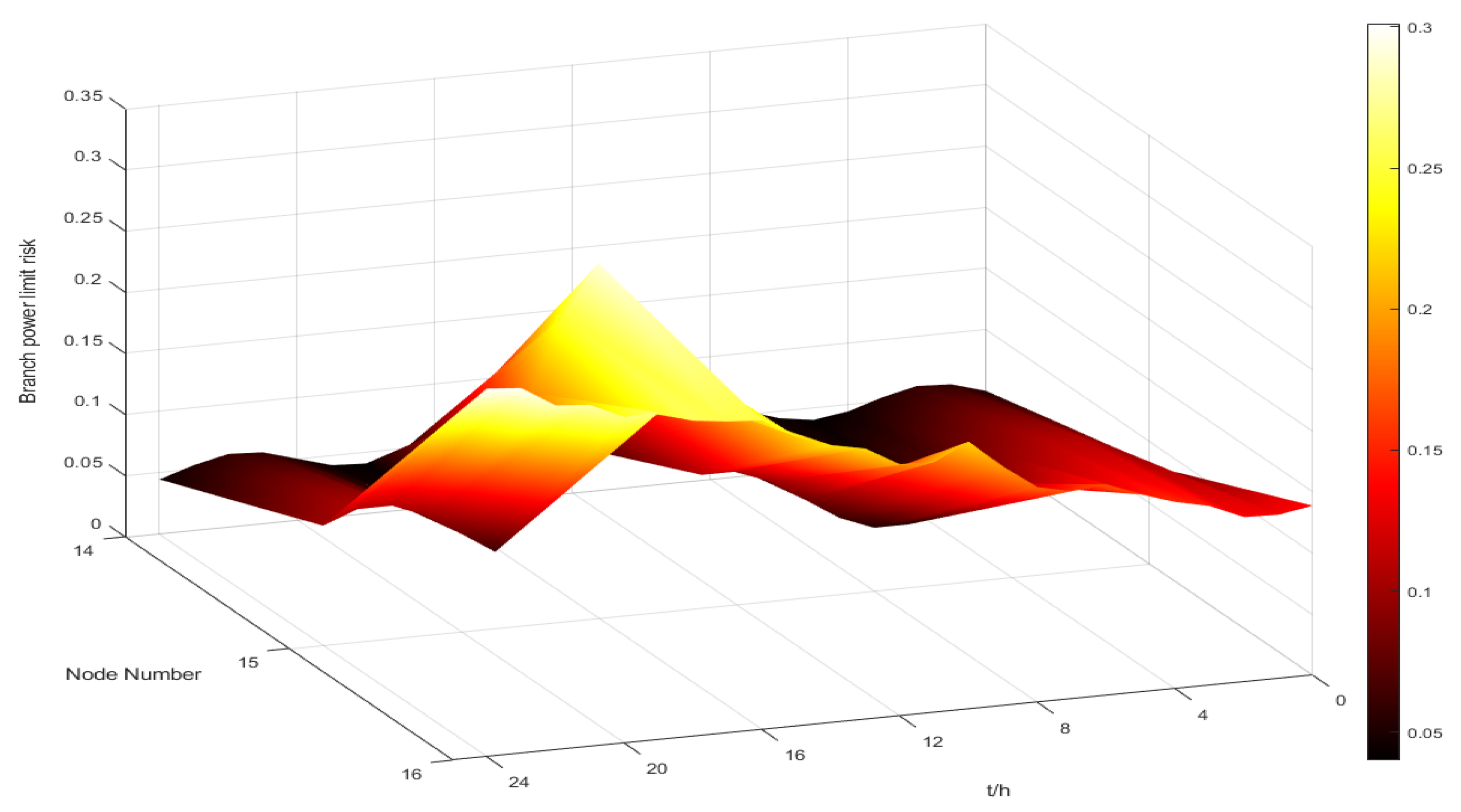
The predicted hourly wind speed sequence is employed as the driving variable for a multi-stage, temporally resolved risk assessment of system operation under extreme gust disturbances. Three representative wind power grid connection nodes—BUS14 (regional coupling point), BUS15 (main load node), and BUS16 (peripheral endpoint)—are analyzed. The temporal evolution of the branch power overlimit risk indicator is assessed using rolling time windows.

Branch Circuit Power Limit Risk

Figure 12 shows the branch circuit power limit risk, and the results indicate:

Figure 12. Branch circuit power limit risk.

(1)

The BUS14 node consistently exhibits the lowest risk values with minimal fluctuations, reflecting strong voltage regulation and power flow diversion capabilities. It can thus serve as a stable anchor point for system operation, demonstrating high robustness against disturbances.

(2)

The BUS15 node shows pronounced volatility, with a notable peak of 0.29 between the 6th and 10th hours, primarily due to high load density and weak voltage support, making it more susceptible to risks during severe wind speed fluctuations.

(3)

The BUS16 node remains in a persistently high-risk state, reaching up to 0.31 in certain intervals. This sustained risk is attributed to its peripheral network position, limited voltage support, and insufficient regulatory resources, which hinder effective short-term mitigation during wind power injections in edge regions.

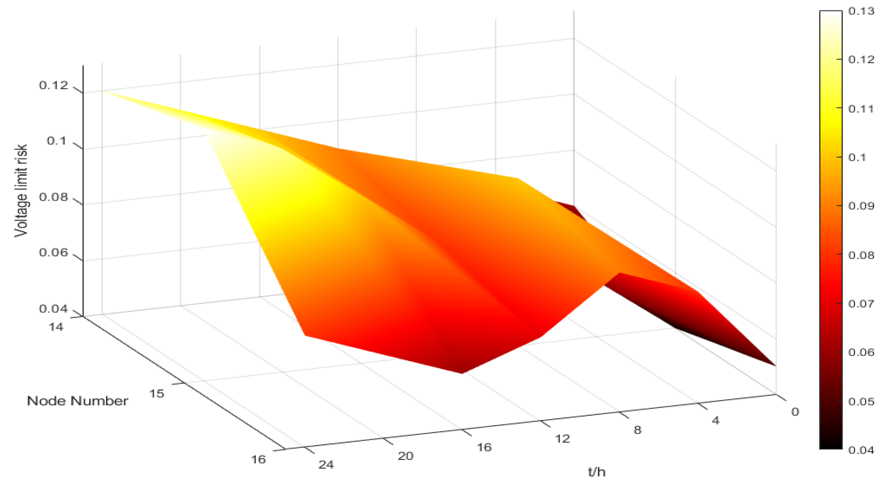
Voltage Limit Risk

Figure 13 shows the Voltage limit risk, and the results indicate:

Figure 13. Voltage limit risk.

(1)

BUS14, the system’s central hub, exhibits stable variations with a “slow start–rapid response” risk pattern. At the 15th hour, intensified wind disturbances raise the risk index to 0.13, indicating strong voltage regulation capacity but notable boundary sensitivity.

(2)

BUS15 follows a three-phase risk profile: trough (<0.04, 0–10 h), surge (peak 0.12, 10–15 h), and stabilization. The surge results from combined wind and load disturbances, underscoring the need for enhanced voltage support.

(3)

BUS16 maintains the lowest overall risk, starting high (>0.08, first 5 h) before converging to ~0.03 as self-balancing power flows restore stability.

(4)

Risk propagation initiates at edge node BUS16 and advances inward to BUS14 and BUS15, illustrating a typical disturbance transmission pattern.

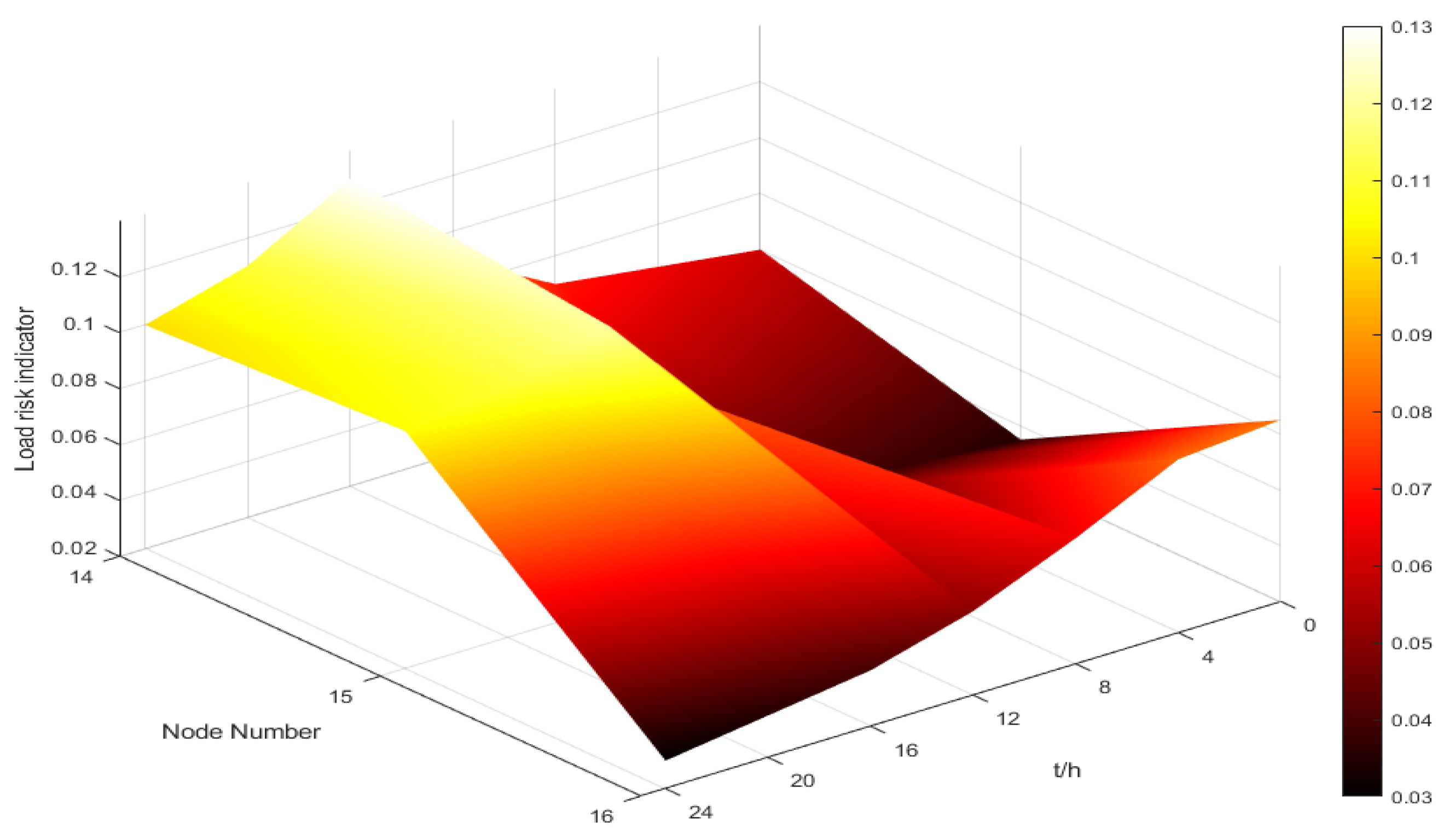
Load Shedding Risk

Figure 14 shows the Load shedding risk, and the results indicate:

Figure 14. Load shedding risk.

(1)

All risk indicators stay below 0.08, indicating sufficient load redundancy under extreme wind disturbances and a well-maintained supply–demand balance.

(2)

BUS14 experiences a sharp risk drop at the 10th hour (0.06 → 0.015), forming a “single-cycle collapse” caused by delayed dispatch response, which temporarily widens the supply gap before rapid recovery.

(3)

BUS15 remains within 0.04–0.07 with minimal fluctuations, reflecting steady-state adjustment. Its central position provides multiple control pathways and high load redundancy, effectively absorbing volatility and supporting higher shares of variable generation.

(4)

BUS16 exhibits a “sawtooth” pattern, with minor declines at 5–10 h and 17–22 h, driven by branch fluctuation propagation and boundary effects. While no direct imbalance occurs, weak coupling of voltage support and load regulation increases cumulative vulnerability.

5.4. Dynamic Response Sensitivity Analysis and Comparison Based on Multidimensional Risk Assessment

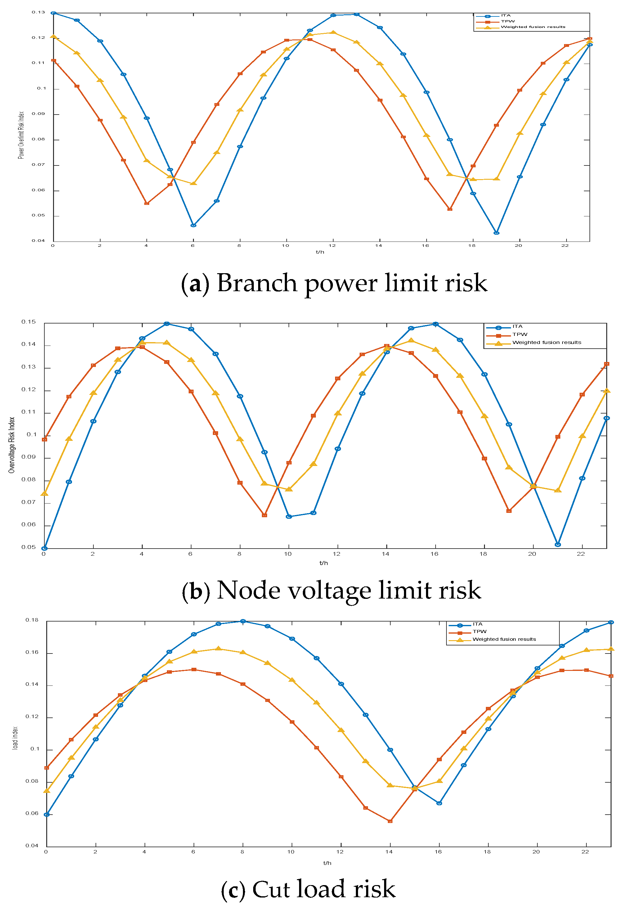
To fully reveal the similarities and differences in the responses of multi-risk assessment methods during system disturbances, this paper further compares the response patterns of branch power overlimit, voltage overlimit, load loss, and three risk indicators in typical time sequence disturbance scenarios. The results are shown in Figure 15.

Figure 15. Node voltage limit risk, branch power limit risk, load shedding risk.

As shown in Figure 15, operational risk indicators from different methods exhibit distinct temporal patterns, reflecting variations in dynamic sensitivity and trend tracking. For branch power overlimit risk, ITA produces sharper peaks during sudden disturbances (6–8 h, 18–20 h), while TPW remains steadier in 12–14 h, indicating respective strengths in early-event detection and long-term evolution tracking. Weighted fusion integrates both, yielding smoother peak transitions and stronger overall representation.

In node voltage overlimit risk, ITA captures early jumps (0–6 h) and TPW emphasizes later fluctuations (14–22 h); fusion reveals delayed peak positions, indicating phase-specific temporal lags. For load loss risk, fusion balances ITA’s rapid response with TPW’s sustained tracking, enhancing regulation under high load-loss conditions. For expected outage duration, ITA is more responsive to early uncertain disturbances, whereas TPW is more stable during system recovery.

5.5. Quantitative Statistical Analysis of Risk Indicators

For each indicator, the mean value, standard deviation and peak-to-average ratio (PAR) were calculated from the same time series used in the risk plots. The results are shown in Table 5.

Table 5. Statistical characteristics of risk indicators.

Indicator	Mean	Standard Deviation	Peak-to-Average Ratio
$R_{CUT}$	0.12	0.05	1.40
$R_{LINE}$	0.22	0.07	2.20
$R_V$	0.27	0.07	2.20

These numerical results are consistent with the qualitative findings. $R_{CUT}$ exhibits the lowest variability, whereas $R_{LINE}$ and $R_V$ show larger fluctuation ranges, indicating higher sensitivity to power-flow and voltage-stability disturbances during extreme gust periods.

To further demonstrate the computational efficiency of the model, this paper divides the computation time into two parts: model training time and risk assessment computation time (Table 6).

Table 6. Computational time of different risk assessment methods.

Method	Training Time (Seconds)	Risk Computation Time (Seconds)	Total Time (Seconds)
BiLSTM-Adaboost-ABKDE	204.43	22.13	233.65
Monte Carlo Simulation	-	125.75	330.18

Training Time: This refers to the time required for the training process of the BiLSTM-Adaboost-ABKDE algorithm, i.e., the time the model spends learning from the training data.

Risk Computation Time: This is the time required for risk assessment after the model completes its predictions, specifically including the calculation of the wind farm’s risk metrics based on the predicted results.

In this study, the training time of the BiLSTM-Adaboost-ABKDE model was 204.43 s, the risk assessment computation time was 22.13 s, and the total time was 233.65 s. Although the model incorporates the Adaboost and ABKDE modules, which increase its complexity, the computational efficiency remains within a reasonable range. In comparison, the traditional Monte Carlo simulation method had a total computation time of 330.18 s, which is significantly higher than that of the BiLSTM-Adaboost-ABKDE model. This indicates that the proposed BiLSTM-Adaboost-ABKDE method has a significant advantage in computational efficiency while also providing higher performance in terms of accuracy. Particularly in practical applications of wind power forecasting and grid risk assessment, the BiLSTM-Adaboost-ABKDE model not only effectively reduces computational costs but also ensures high-precision predictions under extreme conditions, making it more broadly applicable.

6. Conclusions

This study explores the challenges of evaluating wind farm operational risks under extreme gust conditions, primarily including issues such as model insufficiency, the difficulty in balancing accuracy and uncertainty, and the limitations of evaluation perspectives. To address these challenges, this paper proposes a wind power forecasting and multidimensional risk assessment model based on the BiLSTM-Adaboost-ABKDE algorithm framework. The model’s generalization ability and robustness were validated through performance comparisons on the training, validation, and test datasets. Experimental results show that the model exhibits stable RMSE and MAPE values under high-volatility wind speed conditions, demonstrating its adaptability and stability in complex environments.

Moreover, the ensemble learning and adaptive bandwidth mechanism effectively mitigate the impact of data sparsity and sudden fluctuations, showcasing the model’s robustness under small sample sizes and large fluctuations. Compared to traditional BiLSTM, GRU, Transformer, and GAN models, the BiLSTM-Adaboost-ABKDE model shows significant advantages in wind power forecasting, particularly under high volatility and extreme gust conditions. It not only reduces prediction errors but also maintains a high prediction interval coverage. The experimental results validate the model’s superiority and robustness in small-sample and high-volatility data scenarios.

The innovation of this study lies in the introduction of the ITA-TPW weighted fusion method, which not only enhances the temporal feature extraction capability of the BiLSTM model but also addresses the challenges faced by traditional methods in handling wind power forecasting accuracy and risk assessment under extreme gust conditions. The ITA (Integrated Trend Analysis) method captures rapid wind speed variations more accurately by analyzing the time-series trends of wind farm data, while TPW (Time-Series Probability Weighting) effectively handles high-noise data through a weighting mechanism, ensuring the model maintains high stability and accuracy under extreme weather conditions. The introduction of this weighted fusion method enables the model to provide not only wind power forecasts but also quantify prediction uncertainty, offering more comprehensive risk assessment information, thus supporting grid scheduling and wind farm optimization. Quantitatively, on the Hebei case study the proposed method improves the accuracy of the load shedding risk and voltage overlimit risk indicators by 6.15% and 4.79%, respectively, and reduces the total computation time to 233.65 s (204.43 s for model training and 22.13 s for risk assessment), which is lower than the 330.18 s required by the Monte Carlo simulation benchmark.

Although the experimental results show that the model performs well in short-term wind power forecasting, there are still some limitations. First, the experimental dataset is solely from Hebei Province, and it only focuses on short-term wind power forecasting. Although the model performs excellently on this dataset, its applicability in other regions and long-term forecasting scenarios remains unverified. Therefore, future research should incorporate wind power data from different geographic regions and seasons to assess the model’s adaptability and universality under diverse climate conditions. Additionally, although this study focuses on short-term wind power forecasting, future applications could further extend to multi-timescale forecasting, particularly medium- and long-term predictions. By integrating real-time wind speed, wind direction data, and other information, the model’s accuracy and reliability could be further enhanced. Given the model’s strong scalability, future optimization should include improvements to the network architecture, increasing data dimensions, and introducing online learning algorithms to enhance the model’s adaptability and real-time response capability in large-scale wind farms.

Overall, the BiLSTM-Adaboost-ABKDE model proposed in this paper provides solid support for wind farm risk assessment and grid scheduling. However, further optimization and validation are needed for its scalability in cross-regional and long-term forecasting scenarios to ensure its effectiveness in practical applications.