Abstract
The peculiarity of the functioning of modern electric power systems, caused by the presence of renewable energy sources, flexible control devices based on power electronics, and the reduction of the reserve of the transmission capacity of the electric network, increases the relevance of identifying and damping low-frequency oscillations (LFOs) of the electrical mode. This paper presents a comparative analysis of methods for estimating the parameters of low-frequency oscillations. Their applicability limits are shown as well as their peculiarity associated with low adaptability, and time costs in assessing the parameters of the electrical mode with low-frequency oscillations are revealed. A method for the accelerated evaluation of low-frequency oscillation parameters is proposed, the delay of which is ¼ of the oscillation cycle. The method was tested on both synthetic and physical signals. In the first case, the source of data was a four-machine mathematical model of a power system. In the second case, signals of transient processes occurring in a real power system were used as physical data. The accuracy of the proposed method was obtained by calculating the difference between the original and reconstructed signals. As a result, calculated error values were obtained, describing the accuracy and efficiency of the proposed method. The proposed algorithm for estimating LFO parameters displayed an error value not exceeding 0.8% for both synthetic and physical data.
1. Introduction
The development of modern electric power systems (EPSs) is associated with the complication of transient process dynamics [1,2,3]. The introduction of renewable energy sources (RESs), control systems based on power electronics, DC inserts and lines, and distributed generation (DG) have led to a change in EPS inertia and an increase in the probability of low-frequency oscillations (LFOs) [4,5].
LFOs of frequency and power signals are one of the main problems affecting the reliability of EPS operation. The presence of LFOs leads to the need to reduce the flow of active power through the elements of the electric grid by changing the active power of synchronous generators (SGs), which affects the economic efficiency of EPS operation as a whole. In addition, there is a tendency for LFOs to develop with an increase in the amplitude of frequency and active power oscillations, which leads to an increase in the probability of EPS stability loss.
Frequency and active power oscillations are typical for any EPS due to random load measurements, the action of automatic voltage regulators (AVRs), and power system stabilizers (PSSs) after disconnection of an element of the electrical network or SG.
The nature of the emergence and development of LFOs has been studied quite well and frequency ranges have been defined, allowing LFOs to be classified into the following groups [6]:
- Oscillations between SGs within one power plant (2–3 Hz);
- Oscillations of one SG relative to the EPS (0.8–1.6 Hz);
- Oscillations between SG groups (0.2–0.7 Hz).
Based on the group of LFOs, various methods can be used to analyze and eliminate them. The level of oscillation damping in the EPS usually depends on the control by means of a PSS installed on the SG and can vary significantly depending on the current characteristics of the SG and the load. When analyzing the results of damping measurements, periods are often identified during which the damping of oscillations is weak. Weak damping means that the EPS may not be reliable because it is not certain that the dynamic response to subsequent events will be sustained. Such a situation cannot be accurately represented within the dynamic model of the system. Therefore, damping control based on measurements is important to prevent potential threats to reliability before they contribute to the development of a large disturbance. LFOs with different frequencies differ in the danger they pose to EPS stability and in the ways they are damped. Oscillations of individual SGs within a single station are the least dangerous to EPS stability and can be damped by reducing SG power. Oscillations of SGs relative to the EPS are more dangerous and can be damped by disconnecting the SG or reducing its active power. Oscillations between SG groups are the most dangerous.
LFOs are a dangerous phenomenon for the reliability of EPS operation due to their tendency to increase the amplitude and frequency of oscillations, which leads to a loss of stability. In addition, the oscillatory nature of the change in the parameters of the EPS operating mode can provoke mechanical vibrations and increased wear of SGs. Rapid identification of the presence of LFOs and taking preventive measures to dampen them is an important task in the conditions of modern EPSs with reduced inertia and an increased probability of the occurrence of oscillatory electromechanical transient processes.
The main feature of LFO analysis is related to their nonlinear nature and modulation of frequency and amplitude within the oscillation cycle [7]. Despite the active development of LFO analysis methods [8], and the development and implementation of devices for stabilizing oscillations in EPSs by influencing the AVR SG system, the problem of accelerated assessment and determination of minimum control actions (CAs) to eliminate the LFO process remains relevant [9].
The objective of this study is to develop an accelerated LFO parameter estimation method based on orthogonal decomposition of frequency and active power signals for controlling combined EPSs.
The scientific novelty of this study lies in the development of an accelerated method for analyzing LFO parameters with a computational delay of the corresponding quarter of the oscillation. Acceleration of determining the LFO signal parameters is achieved by using a procedure for decomposing the signal into orthogonal components on a calculation window with an adaptively selected width.
2. Current State of the Problem
One of the most common methods of LFO analysis is empirical mode decomposition [10]. This will be designated as Method 1 (M1) The method involves decomposing the signal into mode components with subsequent identification of dominant modes and their parameters. In the course of practical application of M1, the following disadvantages were identified: the inability to isolate modes with close frequencies; complexity of decomposition into dominant modes of narrowband signals; insufficient accuracy when analyzing signals with high-frequency noise components.
To be able to apply M1 in the analysis of LFOs found in real EPSs, modifications of this method were developed:
- Variation mode decomposition (VMD) [11,12];
- Analytical mode decomposition (AMD) [13];
- Improved analytical mode decomposition (IAMD) [14];
- Dynamic mode decomposition (DMD) [15].
To estimate the LFO parameters, a variation mode decomposition method is proposed in [11]. It will be abbreviated M2. The method consists of decomposing the original signal into several modal functions with different central frequencies using a set of adaptive filters. This ensures optimal acquisition of modes and estimates of the reconstructed signal, as well as provision of information on their instantaneous modal characteristics: amplitude, frequency, and attenuation coefficient. To determine the number of eigenmodes, the authors used the Gray Wolves optimization algorithm. During testing of the method on mathematical and physical data, it was determined that in the presence of noise in the original data, the proposed LFO parameter method allows obtaining a smaller error compared to the Prony (PM), Gilbert–Huang, and random decrement methods. In [12], a comparison of the accuracy of the M2, PM, and eigenvalue analysis methods is given. Mathematical data and signals obtained during the recording of technological disturbances in the EPS of Brazil were used for testing. The authors of the study point out the complexity of setting up the M2 method, due to the need to determine the parameters.
One of the varieties of the M1 method is the analytical mode decomposition method, which was used in [13] to analyze the LFO parameters. Further this method will be designed M3. The method allows the signal to be decomposed into two components with frequencies that are multiples of two (bisector frequencies).
To improve the accuracy and efficiency of the M3 method, its improved modification was proposed in [14], which can be used to analyze LFOs in real time. The modification of M3 further will be abbreviated M4. The main problem with the M3 method is to determine the optimal cutoff frequency, which is usually the average frequency value corresponding to neighboring maxima of the Fourier transform. In the M4, it is proposed to use the chaotic particle swarm method to determine the optimal cutoff frequency. The proposed method was tested on mathematical and physical LFO signals. To evaluate LFOs in real time, it is proposed to use a sliding calculation window of 5 s.
The dynamic mode decomposition method was developed as a dimensionality reduction method using the linear Koopman operator and singular value decomposition of the instantaneous measurement matrix [15]. The method will be designed as M5. The M5 is able to automatically determine the dominant modes of an oscillatory process. In [15] M5 was applied to estimate LFO signals obtained during mathematical modeling of transient processes using the Kundur four-machine model [16], the IEEE41 model, and data obtained during a transient process in the New England EPS. The difficulty of using M5 for LFO analysis is related to its the linear nature: for signals with significant nonlinearity, a sharp increase in the error in estimating the parameters of oscillatory processes can be observed.
The following are used as alternative methods based on M1:
- Wavelet transform (WT) [17];
- Empirical wavelets transform (EWT) [18];
- Synchrosqueezed wavelet transforms (SWT) [19];
- Prony transform (PT) [20];
- Improved Hilbert–Huang transform (IHHT) [21];
- Auto-regressive moving average (ARMA) [22];
- Linear predictive code (LPC) [23];
- Adaptive matrix pencil algorithm (AMPA) [24];
- Adaptive total least squares-estimation of signal parameters via rotational invariance techniques (TLS-ESPRIT) [25];
- Principal component analysis (PCA) [26];
- Underdetermined Blind Source Separation Algorithm (UBSS) [27];
- Method of sliding statistical segments (SSS) [28];
- Artificial neural networks (ANNs) [29].
For the LFO analysis, the authors of [17] used wavelet transform with the Morlet mother wavelet. The method will be designed M6. This method was tested on the EPS mathematical model containing six SGs. To determine the accuracy of the proposed method, a comparison with the PM method is used. The authors of the study point out the complexity of selecting the parameters of the developed method (central frequency and bandwidth) and propose an empirical technique for selecting parameters, which in general is not universal.
In [18], a method based on empirical wavelet transform and the Yoshida–Bertekko algorithm is proposed for LFO analysis. Further it will be abbreviated M7. The input data for the LFO parameter estimation method are data from synchronized vector measurement units (PMUs), which are fed to the input of the oscillatory component presence estimation unit based on the Tiger energy operator. This operator estimates the instantaneous energy of the signal and is highly sensitive to oscillatory components in the analyzed signal. When an oscillatory component is detected, the signal is decomposed into mode components using the M7 method, followed by an estimation of the mode parameters using the Yoshida–Bertekko algorithm. Synthetic and real measurements were used to test the method. Comparison of the M7 method results with PM and M2 confirmed the efficiency and high accuracy of the proposed method.
The authors of [19] proposed the synchrosqueezed wavelet transforms method for analyzing multicomponent signals with oscillatory components for LFO analysis. Below it will be abbreviated M8. Unlike the wavelet transform, M8 prevents the phenomenon of spectrum spreading. The technique was tested on mathematical and physical signals. The proposed algorithm demonstrates high efficiency in analyzing signals that are superposition of a small number of components that are well separated in the time-frequency plane. However, its success is conditioned by strict requirements for signal regularity and smoothness, including restrictions on the rate of change of amplitudes and instantaneous frequencies. The significant dependence of the results on the choice of the key parameter ϵ complicates optimization. The algorithm is limited to cases with a relatively simple internal signal structure and loses effectiveness with increasing spectral density or the presence of abrupt changes in the signal, which narrows the range of possible applications.
In [20], a comparison of LFO parameter estimation using Prony transform, the Steiglitz–McBride algorithm, and the effect number analysis method is presented. In the future this method will be designed M9 (PT). Transient signals obtained for four EPS models of different configurations were used as the initial data for LFO estimation. A series of numerical experiments yielded a smaller LFO estimation error for M9 compared to the other methods considered. The three algorithms discussed in this article share common drawbacks: the efficiency of all methods decreases with increasing system complexity, especially with multiple weakly damped electromechanical oscillations; the reconstruction of model zero points is less accurate than pole identification; and the choice of an appropriate model order and the need to take numerical stability into account impose additional limitations on their practical application.
In [21], improved Hilbert–Huang transform method was used for LFO analysis, which is aimed at eliminating the mode shift problem by using the symmetric extremum mapping procedure. Further the method will be abbreviated M10. This method allows one to minimize end effects. The algorithm used to analyze LFO in EPS suffers from several limitations. First, the empirical decomposition method causes an end-of-line effect, leading to incorrect instantaneous values at the signal edges and the appearance of spurious internal modes. Second, the problem of mode mixing arises when a single internal mode includes components of different scales or similar scales are distributed across different modes, complicating physical interpretation. These shortcomings lead to a decrease in the accuracy of the analysis and require further refinement of the algorithm.
The work [22] is devoted to the application of Auto-regressive moving average method for LFO analysis. In the future it will be designed M11. The testing was performed on synthetic data and real LFO records. M9 was used to compare the accuracy of the method. The proposed algorithm faces several key challenges. First, the quality of the estimated mode parameters depends significantly on the data block size: for small block sizes, errors arise due to the low accuracy of the autocorrelation matrix calculations, which negatively impacts the results of both the frequency and the mode attenuation degree estimation. An additional challenge arises from the correct choice of model order, which is expressed by the number of equations used: insufficient order leads to underdetermination of the problem, while excessive order overloads the system and increases the error rate. Finally, the attenuation index is particularly difficult to accurately measure, since with a fixed block size, this characteristic is estimated less reliably than the mode frequency, creating significant obstacles to an objective assessment of the system’s state.
The authors of [23] used linear predictive code method to determine the LFO parameters in real time. Further it will be designed M12. The testing was performed on synthetic signals without noise and emissions. The main problem with the proposed method is its high sensitivity to the length of the recorded data: small record sizes lead to significant errors in calculating correlation matrices, which negatively impacts the accuracy of frequency and mode attenuation estimates. Furthermore, an insufficiently precise choice of model order (number of equations) can lead to either an underestimation of system parameters or an increase in calculation errors. It is also noted that the algorithm struggles with separately estimating the fast and slow components of oscillations: the fast component is estimated more accurately, but a larger data volume is required to reliably estimate slowly decaying modes, which can slow down the process of real-time anomaly diagnostics. Thus, despite the potential advantages of the method, its application is limited by the need for careful parameter selection and the large volume of measurement data required.
In [24], the adaptive matrix pencil algorithm was used to estimate the LFO parameters. In the future it will be abbreviated M13. The advantage of the method is the automatic selection of dominant modes of the oscillatory process and the efficiency of suppressing noise and spikes in the original measurements. Synthetic signals obtained by calculating transient processes in the Kundur model with different values of the signal-to-noise ratio were used for testing. M9 was chosen for comparison of the proposed method. The algorithm proposed in this article is highly sensitive to the duration of the data recording window: reducing the observation duration leads to a noticeable degradation in the quality of the correlation analysis and a decrease in the accuracy of LFO parameter estimation. Optimal selection of the model order is also a critical issue, as an incorrectly chosen number of equations causes serious calculation errors. Another significant drawback is its increased sensitivity to noise: high levels of interference significantly reduce the reliability and accuracy of oscillation mode identification. Separate processing of fast and slow components necessitates an increase in the measured signal length to improve the accuracy of slowly decaying mode estimation, further complicating real-time diagnostics. Authors of [24] for LFO analysis earlier in [25] considered the use of adaptive total least squares-estimation of signal parameters via rotational invariance techniques. Future it will be designed M14. The authors propose a two-stage procedure consisting of a block of filtering the original data and a block of estimating the LFO parameters. Testing was performed on the Kundur model.
In [26], a method for calculating LFO parameters based on principal component analysis was proposed. This method will be designed M15. The IEEE14 model was used for testing. The main drawback of the algorithm is the difficulty of processing heterogeneous data coming from distributed generators and a variety of sensor types. Interpreting interactions between different areas of the system becomes difficult as its scale and complexity increase. Combining data from regional monitoring centers to obtain a comprehensive picture of system behavior is also challenging. Further research and the development of new metrics are needed to address these limitations and improve the effectiveness of the method.
The authors of [27] used Underdetermined Blind Source Separation Algorithm to analyze LFO. The LFO start time is determined by calculating the signal energy. The method in the future will be abbreviated M16. An analysis of experimental data and computer simulations revealed a key limitation of the proposed method: its insufficient robustness to intense noise, typical of real-world power system operating conditions. This leads to a reduction in the accuracy and reliability of separating oscillation modes with adjacent frequencies. Although the algorithm outperforms classical approaches such as the Prony method in noise suppression, the problem of mode superposition remains, reducing the overall identification accuracy.
In [28], a method for estimating LFO parameters based on Method of sliding statistical segments was proposed. Further it will be designed M17. The method involves determining the LFO signal extremes by using the sliding parabola method on calculation windows of a given width. The method delay is half the LFO oscillation cycle. The method was tested on real LFO measurements occurring after a technological failure near a large power plant. LFO hazard criteria were proposed.
Method based on artificial neural networks was used in [29] to estimate the LFO parameters. Further it will be abbreviated M18. The data sample was formed using the procedure of numerical modeling of transient processes in the Kundur model and the results of estimating the LFO parameters using the M2 method. Despite the positive aspects of this approach, there are significant limitations. The most important issue is the complex tuning of hyperparameters, such as the number of layers, the number of neurons, and activation functions, which reduces the method’s versatility. High computational resource requirements, including memory and training time, make implementation challenging under resource constraints. The quality of data pre-training plays a crucial role: poor pre-training significantly reduces prediction accuracy. Due to their “black box” nature, neural networks make it difficult to interpret decisions, weakening confidence in the results. Finally, a system trained on a specific set of configurations adapts poorly to new situations, limiting its application in the ever-changing electric power industry.
In work [30], authors propose a new type of stabilization device designed to damp LFO in EPS systems with significant power electronics conversion devices. With advances in virtual synchronous generator technology, authors in work [31] suggest a damping system for LFO in EPS incorporating virtual SG units. Work [32] employs the DMD algorithm for assessing LFO parameters, validated using simulation data from the IEEE39 test model. Researchers in [33] utilize a harmonic state-space model for analyzing LFO phenomena. To identify the source of LFO in EPS, researchers in [34] employ a combined Prony’s method and Fast Fourier Transform approach [35].
Of the LFO analysis methods considered, four stand out for which calculations are used on sliding windows of limited width: M4, M7, M12 and M5. For the remaining methods, the LFO parameters are estimated under conditions of consideration of the full-time interval of the LFO existence, which complicates their use in EPS control systems. The works considered do not use adaptive selection of the width of the LFO estimation calculation window.
Table 1 provides a comparison of LFO analysis methods in terms of the time interval under consideration. In Table 1, the advantages of the method are indicated by the symbol «(+)», and its disadvantages by the symbol «(−)».

Table 1.
Analysis of LFO parameter estimation methods.
To increase the speed of LFO estimation in EPS conditions with reduced inertia due to the introduction of RES, this study presents an accelerated method for estimating the frequency and magnitude of the LFO, which allows, on a sliding calculation window, to obtain an estimate of the LFO parameters with a computational delay of the corresponding quarter of the oscillation period. The work also includes testing on both synthetic and physical data, which allows one to evaluate the reliability of the proposed method in conditions of noise in the original data. The scientific novelty of the proposed method lies in the acceleration of the LFO parameter estimation by using orthogonal decomposition of the signal under consideration and adaptive tuning of the base frequency. The computational delay of the method proposed in this study corresponds to a quarter of the LFO oscillation period, which exceeds the performance of the methods considered in Table 1.
3. Method for Accelerated LFO Parameter Estimation
Based on the analysis of the considered methods, a method for accelerated estimation of the frequency and magnitude of an oscillatory signal on sliding windows of limited width was developed. The method consists of sequential execution of operations for processing signals from phasor measurement units (PMUs). This source of measurements allows obtaining information with high accuracy and a time delay corresponding to the period of the industrial frequency [29]. Figure 1 shows a flowchart of the proposed method for accelerated estimation of LFO parameters. The LFO parameters obtained during accelerated evaluation are understood to be the magnitude and frequency of the signal with the presence of a low-frequency component.
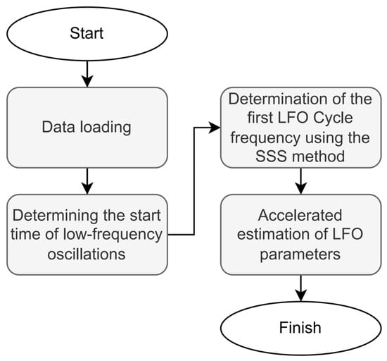
Figure 1.
Flowchart of the accelerated LFO evaluation methodology.
The signal derivative analysis method, which was used to identify the onset of a short circuit (SC) [36], is used to identify the LFO. The first LFO cycle value is estimated using the SSS method for adaptive selection of the sliding calculation window value. The SSS method is based on the mathematical problem of searching for a local extremum of a signal using calculations on sliding windows. Using this approach, the minimums and maximums of the signal with the presence of an LFO are determined, from which the magnitude and frequency of the signal are calculated. A more detailed description and testing of the SSS method is presented in a previous study [28].
The width of the sliding calculation window is taken to be equal to one quarter of the first LFO cycle time. A modified method [37] is used for accelerated estimation of the PER LFO, the flowchart of which is shown in Figure 2.
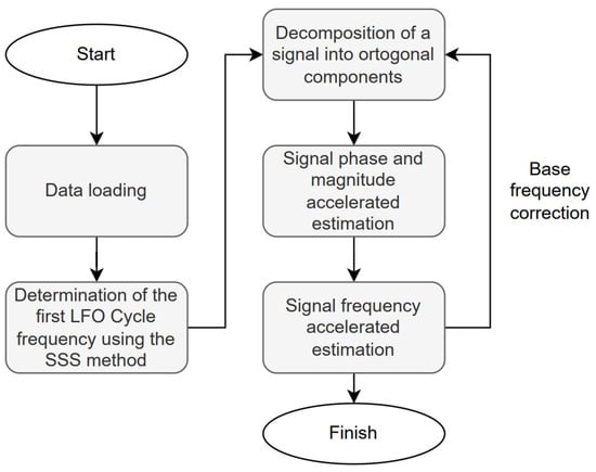
Figure 2.
LFO time series processing process.
After identifying the start of the LFO, the base frequency and the calculation window are estimated using the SSO method (in Figure 2, the definition of the initial approximation of the base frequency and the width of the calculation window is highlighted by a dotted line). Then, the analyzed signal is decomposed into orthogonal components:
where x(t) is the analyzed signal; a0(t) is the constant component of the signal; w(t) is the base frequency of the signal; a(t), b(t) are the coefficients of the first terms of the Fourier series.
To obtain the coefficients of model (1), a multiparameter model is used, which describes a random non-stationary process and, in general form, can be represented as a decomposition of a regular component (trajectory) and an irregular (random) component [35]. According to Kolmogorov’s theorem, any continuous function of many variables can be expressed as a superposition of continuous functions of one variable and addition. In turn, the function of the independent parameter x can be represented as a sum of elementary (basis) functions of the same parameter, associated with connection coefficients and parameters of these basis functions. The multiparameter model can be written as follows:
where n is number of independent parameters, x is independent parameters, f is elementary function, a is connection coefficients, k is number of basis functions for the j-th independent parameter, H is parameters of the basis functions, l–basis function number.
Then, to find the sought-after coefficients a, it’s necessary to minimize the following expression:
where Y—measurements of the dependent parameter at time ti.
The solution of task (3) coincides with the solution of the system of equations:
where A и Ψ—matrices obtained after transforming expression (3), and a—vector of the desired coefficients.
To solve this problem, it is advisable to apply a non-recurrent learning algorithm, which is a modification of Gauss’ method for solving systems of normal linear equations. The usual difficulty in solving equation systems like (4) lies in the fact that if the determinant of matrix A equals or approaches zero, it complicates the use of conventional methods. Poor conditioning of the system arises because elements of the matrix are chosen arbitrarily and thus do not satisfy the condition of “strong” convergence on the training sample. Given the possibility of matrix A being singular, instead of finding solutions to Equation (4), we will seek solutions to a system of inequalities.
An advantage of the multiparameter model algorithm is that it guarantees small residuals, regardless of the number of “excluded” equations. This result is achieved due to taking into account the specific nature of the system, where both the coefficients and the right-hand side have the form given by Equation (4). Thus, the described multiparameter algorithm exhibits absolute computational stability and selective properties essential for solving problems of this kind.
The LFO parameters are defined as follows:
where A(t) is the signal magnitude; φ(t) is the signal phase.
To calculate the signal frequency, a procedure of numerical differentiation on sliding windows of the phase signal is used. The correction of the base frequency of the signal w(t) is performed at each step of the calculation window by setting the calculated frequency value from the previous step as the base frequency.
The accuracy of determining the LFO parameters is assessed by calculating the signal recovery error:
where ∆x(t) is the difference between the original and reconstructed signals.
The selection of the sliding calculation window value is determined by a quarter of the LFO oscillation period determined at the initialization stage using the SSS method. The value of the calculation window is adaptive depending on the value of the LFO cycle identified at the beginning of the transient process. In the process of estimating the LFO parameters, the value of the calculation window is adjusted depending on the value of the base frequency adjustment in expression (1).
4. Testing the Method of Accelerated LFO Parameters Estimation
To test the method, two types of data are used: synthetic (obtained as a result of mathematical modeling of the transient process in the EPS model) and physical (obtained during the registration of transient processes occurring in a real EPS). The choice of synthetic and physical data sources is justified by the availability of data and the sufficiency of the EPS mathematical model to synthesize LFOs. For synthetic data, standard mathematical models were utilized: the four-machine Kundur model and the modified IEEE24 model. The parameters of these employed EPS mathematical models are standard and available in open-source references.
4.1. Synthetic Data
A mathematical model of an EPS consisting of four SGs was used as a source of synthetic data. This model was proposed by the Indian researcher P. Kundur [15] to study dynamic processes in an EPS. Figure 3 shows the diagram of the used mathematical model. The SG and load parameters are given in Table 2 and Table 3. A detailed description of the used EPS model is presented in [15]. The following notations are given in Table 2: Xd—direct-axis synchronous reactance; Xq—quadrature-axis synchronous reactance; Xd′—direct axis transient impedance; Xd″—direct axis subtransient impedance; Xq′—quadrature axis transient reactance; Xq″—quadrature axis subtransient reactance; Ra—armature resistance; Td0′—direct-axis transient time constant; Tq0′—quadrature axis transient time constant; Td0″—direct-axis subtransient time constant; Tq0″—quadrature axis subtransient time constant; H—inertia constant.
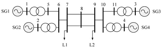
Figure 3.
Kundur’s EPS model.
Table 2.
SG parameters.
Table 3.
Load parameters.
All SGs are modeled taking into account the AVR, system stabilizers and turbine speed control devices. To model the LFO, a transient process with a three-phase short circuit in node 8 lasting 0.1 s with disconnection of PSS SG1 and SG2 was considered. The signals sampling frequency was taken to be 60 Hz, which corresponds to the alternating current frequency used in the Kundur model.
Figure 4 shows the active power signal along one of the parallel lines 7–8, the LFO magnitude signal, and the LFO frequency signal. In the first cycle, the signal frequency estimated using the SSS method was 0.5 Hz, and the sliding calculation window was 0.5 s.
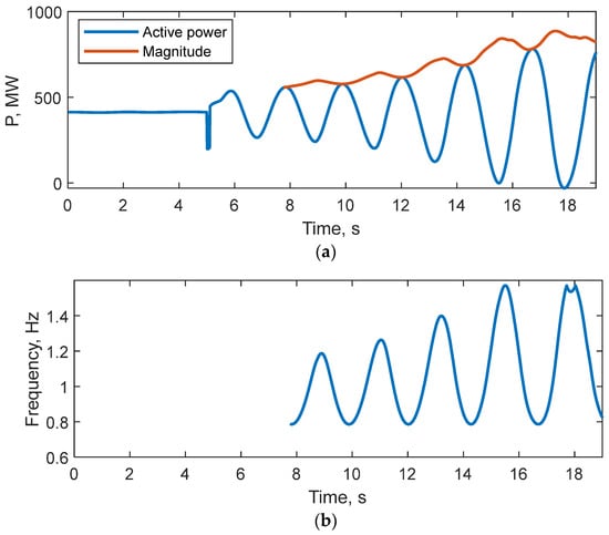
Figure 4.
The result of Kundur’s model LFO parameter estimation: (a) LFO active power and magnitude signal; (b) LFO frequency signal.
Table 4 shows the statistical parameters of the signal recovery error (7) based on the calculated LFO values.
Table 4.
Parameters for assessing the accuracy of synthetic signal reconstruction (Kundur model).
The average difference between the original and reconstructed LFO signal was 1.6 MW or 0.3% of the original active power.
For testing on synthetic data, a more complex IEEE24 model [36,37] was used. For the IEEE24 model modification, power generation in nodes 1, 2 and 7 is carried out using wind generators (WG). The SGs are modeled taking into account the operation of turbine models, automatic excitation regulator and system stabilizer. In the IEEE24 model used, all SGs are connected to the power grid via block step-up transformers. SG 16 models the connection to the external EPS. The model graph is shown in Figure 5. The SG parameters are presented in Table 5, and the load parameters are given in Table 6. The notations adopted in Table 5 correspond to the notations from Table 2. In Table 6, Vmax denotes the maximum voltage of a node, Vmin denotes the minimum voltage of a node.
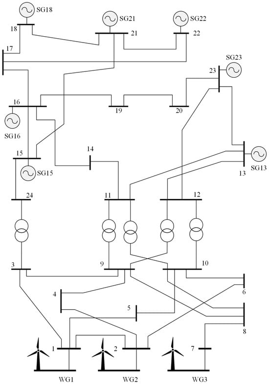
Figure 5.
IEEE24 model diagram.
Table 5.
SG parameters.
Table 6.
Parameters of IEEE24 model nodes.
The IEEE24 mathematical model is one of the standard models for studying electromechanical transient processes in EPS, its detailed description can be found in studies [36,37]. To generate the LFO, a three-phase SC to ground of 0.2 s duration on line 14–15 was simulated in the IEEE24 mathematical model. The change in active power, magnitude, and frequency of the LFO on line 22–21 are shown in Figure 6.
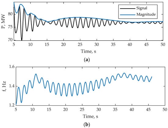
Figure 6.
The result of IEEE24 model LFO parameter estimation: (a) LFO active power and magnitude signal; (b) LFO frequency signal.
Table 7 presents the results of the evaluation of the accuracy of the LFO parameters calculation.
Table 7.
Parameters for assessing the accuracy of synthetic signal reconstruction (IEEE39 model).
During testing of the proposed method for estimating LFO parameters on the EPS mathematical models, average error values of 0.3% and 0.16% were obtained for the Kundur and IEEE24 models, respectively.
4.2. Phisical Data
To test the method of accelerated estimation of LFO parameters, we used physical data obtained during transient processes of the SG power plant [38], the diagram of which is shown in Figure 7. All considered signals with the presence of LFO were obtained as a result of island operation of the power plant. The power plant consists of 10 SGs, the parameters of which are given in Table 8. All the considered power units use the same type of block transformers. All SGs use the same equipment: both the exciter and the excitation regulator. The connection of the considered power plant with the external EPS is carried out due to three 110 kV transmission lines and four 330 kV transmission lines. Figure 7 shows the graphs of the change in the active powers of SG3 and SG7, as well as the change in frequency on the 330 kV buses during a technological disturbance with the presence of LFO. Figure 8, Figure 9 and Figure 10 show the values of active powers and the estimated parameters of the SG7 LFO during various technological disturbances. Table 9 shows the parameters of the signal recovery error based on the calculated LFO values.
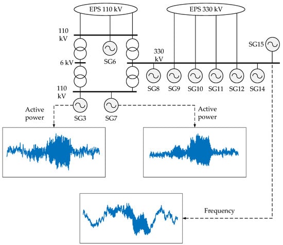
Figure 7.
Scheme of the power plant under study.
Table 8.
Rated parameters of SGs.
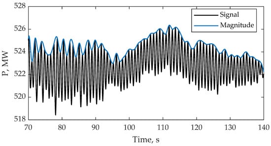
Figure 8.
The result of Signal 1 LFO magnitude estimation.
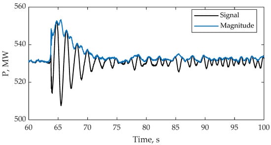
Figure 9.
The result of Signal 2 LFO magnitude estimation.
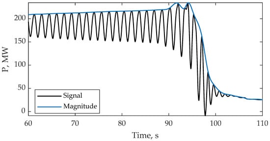
Figure 10.
The result of Signal 3 LFO magnitude estimation.
Table 9.
Parameters for assessing the accuracy of physical signals reconstruction.
During the numerical experiment, synthetic and physical LFO signals were considered. For the synthetic signal obtained during the simulation of the transient process in the four-machine Kundur model, the maximum error in signal reconstruction based on the calculated parameters of the LFO signals was 0.8% of the pre-emergency value of the active power. For testing on physical data, three active power signals recorded during the transient processes in a real EPS were considered.
4.3. Comparison of the Proposed Method with SSS and VMD
In a previous study [28], the SSS method was proposed for estimating the frequency and amplitude of the LFO, which is based on the procedure for determining local extremes of the oscillatory signal with their subsequent use for calculating the LFO parameters. In this case, the amplitude and frequency values are determined by the following equations:
where A is the signal magnitude; f is the signal frequency; C is the coordinate along the vertical axis (of values) of the midpoint of the vertical segment connecting some local extremum and the segment connecting the extrema adjacent to it; y1 and y2 are the coordinates along the vertical axis (of values) of adjacent extrema; x1 and x2 are the coordinates along the horizontal axis (of time) of two consecutive opposite extrema.
The SSS method has low computational complexity with a delay of LFO parameter estimation of half the oscillation period. The accuracy and performance of the SSS method were discussed in detail in a previous study [28]. This section discusses a comparison of the results of the accuracy of LFO signal restoration using the parameters determined by the accelerated method discussed in this article and the SSS method.
Table 10 shows comparisons of the results of LFO signal restoration using the proposed accelerated method, the SSS and VMD methods. The SSS and VMD algorithms were chosen for comparison for the following reasons: the proposed accelerated algorithm for estimating LFO partners is a development of the SSS algorithm aimed at increasing its speed and accuracy, the VMD algorithm is one of the most flexible and effective algorithms for determining LFO parameters.
Table 10.
Comparison of the results of the proposed accelerated method for estimating LFO parameters, SSS and the VMD method.
The accuracy of LFO signal reconstruction based on parameters calculated by the SSS method is on average 68% lower compared to the accelerated method proposed in this article. The low accuracy of the SSS method is due to the insufficient accuracy of determining the LFO signal extremum under conditions of noise in the original data and distortion of the signal shape. The results of LFO estimation parameters by the proposed method and VMD are close; however, the considered methods are characterized by different time delays, reaching for VMD the full interval of LFO existence.
The proposed method of accelerated LFO parameter estimation has filtering properties due to the signal approximation by Equation (1) on a sliding window of limited width. As a result, the influence of noise in the data for the proposed accelerated LFO parameter estimation method is not as critical as for the SSS method. Depending on the width of the calculation window, it is possible to increase or decrease the filtering properties, which provides a certain flexibility when using the proposed method of accelerated LFO parameter estimation for signals with noise.
The choice of the width of the calculation window of the proposed method depends on the requirements for speed and noise of the initial data. Figure 2 shows a block diagram of the proposed method, in which the width of the calculation window is determined adaptively on the first LFO cycle using the SSS method. In general, the width of the calculation window can be limited depending on the noise of the initial data. Setting the limits of the width of the calculation window can be done by experts or during a preliminary analysis of the characteristics of the signals under consideration. The development of a method for automatically determining the width of the calculation window is a direction for future research.
4.4. Assessment of the Impact of Noise in the Raw Data on the Accuracy of Estimating LFO Parameters
To assess the effect of noise on the results of LFO parameter estimation, synthetic data used in Section 4.1 with the application of the IEEE24 mathematical model were subjected to noise distortions at different amplitude levels. The results of evaluating the accuracy of determining LFO parameters depending on the level of noise in the data are presented in Table 11.
Table 11.
Analysis of the influence of noise in the raw data on the accuracy of determining LFO parameters.
Adding noise to the raw data within a range from 0 to 20 dB leads to an increase in the average value of Δx by 0.07 MW, which is a high result demonstrating robustness of the developed method against noise. Depending on the noise level, the size of the calculation window can be adjusted, increasing its filtering properties.
5. Discussion
Implementation of the proposed accelerated analysis method for correction in actual EPS could be realized through utilization of data from Phasor Data Concentrators (PDC), aggregating information received from PMUs installed across the considered EPS network. Upon identification of the start time and parameters of LFO events, such information may be leveraged to select and implement control actions aimed at dampening LFO effects via adjustments to PSS or AVR settings. Another potential application involves manual analysis of LFO phenomena by experts responsible for manually controlling or configuring equipment managing EPS operational modes.
Figure 11 illustrates a possible architecture for implementing the proposed methodology for rapid assessment of LFO parameters.
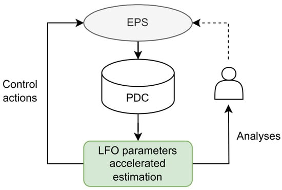
Figure 11.
Architecture for integrating the accelerated algorithm for estimating LFO parameters into EPS management structures.
When implementing the developed method for accelerated evaluation of LFO parameters within the framework of individual studies, the following tasks must be solved:
- Developing the architecture of the system for collecting and analyzing signals describing the change in active power, currents and frequency during the LFO process. This architecture must be fault-tolerant, scalable and fast;
- Determining the permissible sampling frequencies and update times for signals defining the electrical mode parameters, allowing the LFO parameters to be estimated with acceptable speed and accuracy;
- Developing a method for selecting and implementing control actions that ensure LFO damping;
- Determining the list of functional capabilities required to analyze LFO parameters in autonomous mode;
- Determining the optimal number of PMUs required for a comprehensive analysis of the oscillatory component of low-inertia EPS with a significant share of wind power plants and control systems based on power electronics.
- Developing requirements for communication channels between the control system and control objects in the EPS.
6. Conclusions
This review and analysis of studies aimed at developing methods for identifying LFO parameters showed that most methods use the entire interval of existence of LFO parameters to estimate the parameters of the oscillatory process, which limits the possibility of applying the methods to solving EPS control problems.
A method for accelerated LFO parameter estimation is proposed, providing a computational delay equal to a quarter of the oscillation cycle. To ensure adaptability, a procedure for determining the initial value of the base frequency is used, followed by its refinement at each step of the sliding calculation window. The initial approximation of the base frequency is performed using the SSS method, which provides a delay in obtaining the LFO parameters in one oscillation cycle. Due to the use of simple computational operations in the proposed method for estimating LFO parameters, there is no expectation of high computational complexity when working with large volumes of data during practical implementation in real-world EPSs. However, a more thorough investigation into the computational complexity of this method and validation of its performance in real-time operation remains a subject for future research. The proposed algorithm for estimating LFO parameters with an error value not exceeding 0.8% for both synthetic and physical data.
The proposed method for accelerated LFO parameter estimation was tested on the following EPS mathematical models: the four-machine Kundur model and IEEE24. In the used EPS mathematical models, SGs were modeled taking into account the AVR and PSS devices. To estimate the accuracy of calculating the LFO magnitude and frequency, a method for restoring the signal from the calculated parameters is proposed.
The following areas can be identified as areas for future research:
- Testing the proposed accelerated LFO estimation method on a real-time simulator [39,40,41] in order to determine the hardware delay required to perform arithmetic operations on a sliding calculation window;
- Development of an accelerated method for determining the LFO source [42];
- Development of a methodology for determining the volumes of control actions for LFO damping [43,44,45,46];
- Development of a method for automatically determining the width of the design cone depending on the noise level in the initial data.
- The developed algorithm is universal and independent of the applied EPS mathematical model. For further detailed study of the method, it is planned to test it on IEEE39 and IEEE118 EPS mathematical models.
Author Contributions
All authors have made valuable contributions to this paper. Conceptualization, M.S. (Mihail Senyuk) and S.B.; data curation, S.B.; formal analysis, I.Z., M.S. (Murodbek Safaraliev) and S.B. investigation, M.S. (Mihail Senyuk) and I.O.; methodology, I.Z., M.S. (Murodbek Safaraliev) and S.B.; project administration, M.S. (Murodbek Safaraliev); resources, I.Z. and S.B.; software, M.S. (Mihail Senyuk), I.O. and S.B.; supervision, I.Z.; validation, M.S. (Mihail Senyuk) and S.B.; writing—original draft, M.S. (Mihail Senyuk), S.B. and I.O.; writing—review and editing, I.Z., M.S. (Murodbek Safaraliev) and I.O. All authors have read and agreed to the published version of the manuscript.
Funding
This research received no external funding.
Data Availability Statement
The original contributions presented in this study are included in the article material; further inquiries can be directed to the corresponding author.
Acknowledgments
The research funding from the Ministry of Science and Higher Education of the Russian Federation (Ural Federal University Program of Development within the Priority-2030 Program) is gratefully acknowledged.
Conflicts of Interest
The authors declare no conflicts of interest.
Abbreviations
| AMPA | Adaptive matrix pencil algorithm |
| TLS-ESPRIT | Adaptive total least squares-estimation of signal parameters via rotational invariance techniques |
| ANN | Artificial neural networks |
| AVR | Automatic voltage regulator |
| ARMA | Auto-regressive moving average |
| CA | Control action |
| DG | Distributed generation |
| DMD | Dynamic mode decomposition |
| EPS | Electrical power system |
| EMD | Empirical mode decomposition |
| VMD | Empirical mode decomposition |
| EWT | Empirical wavelet transform |
| IHHT | Improved Hilbert–Huang transform |
| IAMD | Improved variational modal decomposition |
| LPC | Linear predictive code |
| LFO | Low-frequency oscillation |
| PMU | Phasor measurement unit |
| PSS | Power system stabilizer |
| PCA | Principal component analysis |
| PDC | Phasor data concentrator |
| PM | Prony’s method |
| PT | Prony’s transform |
| RES | Renewable sources of energy |
| SC | Short circuit |
| SSS | Sliding statistical segments |
| SG | Synchronous generator |
| SWT | Synchrosqueezed wavelet transforms |
| UBSS | Underdetermined Blind Source Separation |
| VMD | Variational mode decomposition |
| WT | Wavelet transform |
References
- Wu, Y.; Ge, L.; Yuan, X.; Fu, X.; Wang, M. Adaptive Power Control Based on Double-layer Q-learning Algorithm for Multi-parallel Power Conversion Systems in Energy Storage Station. J. Mod. Power Syst. Clean Energy 2022, 10, 1714–1724. [Google Scholar] [CrossRef]
- Madurasinghe, D.; Venayagamoorthy, G.K. Distributed Dynamic Security Assessment for Modern Power System Operational Situational Awareness. IEEE Access 2024, 12, 147991–148010. [Google Scholar] [CrossRef]
- Ouyang, J.; Yu, J.; Long, X.; Diao, Y.; Wang, J. Coordination Control Method to Block Cascading Failure of a Renewable Generation Power System Under Line Dynamic Security. Prot. Control Mod. Power Syst. 2023, 8, 12. [Google Scholar] [CrossRef]
- Wu, G.; Sun, H.; Zhao, B.; Xu, S.; Zhang, X.; Egea-Alvarez, A.; Wang, S.; Li, G.; Li, Y.; Zhou, X. Low-Frequency Converter-Driven Oscillations in Weak Grids: Explanation and Damping Improvement. IEEE Trans. Power Syst. 2021, 36, 5944–5947. [Google Scholar] [CrossRef]
- Li, Y.; Fan, L.; Miao, Z. Wind in Weak Grids: Low-Frequency Oscillations, Subsynchronous Oscillations, and Torsional Interactions. IEEE Trans. Power Syst. 2020, 35, 109–118. [Google Scholar] [CrossRef]
- Gupta, D.P.S.; Sen, I. Low frequency oscillations in power systems: A physical account and adaptive stabilizers. Sadhana 1993, 18, 843–868. [Google Scholar] [CrossRef]
- Kovalenko, P.Y. Comparing the approaches to the measurements-based express-analysis of low-frequency oscillations in power systems. In Proceedings of the 2017 IEEE 58th International Scientific Conference on Power and Electrical Engineering of Riga Technical University (RTUCON), Riga, Latvia, 12–13 October 2017; pp. 1–4. [Google Scholar] [CrossRef]
- Bi, J.; Sun, H.; Xu, S.; Song, R.; Zhao, B.; Guo, Q. Mode-based Damping Torque Analysis in Power System Low-frequency Oscillations. CSEE J. Power Energy Syst. 2023, 9, 1337–1347. [Google Scholar] [CrossRef]
- Xue, T.; Zhang, J.; Bu, S. Inter-Area Oscillation Analysis of Power System Integrated With Virtual Synchronous Generators. IEEE Trans. Power Deliv. 2024, 39, 1761–1773. [Google Scholar] [CrossRef]
- Cai, X.; Shu, Z.; Deng, J.; Yang, L.; Zhou, N.; Cheng, S.; Tao, X. Location and Identification Method for Low Frequency Oscillation Source Considering Control Devices of Generator. In Proceedings of the 2018 5th International Conference on Information Science and Control Engineering (ICISCE), Zhengzhou, China, 20–22 July 2018; pp. 818–827. [Google Scholar] [CrossRef]
- Liu, L.; Wu, Z.; Dong, Z.; Yang, S. Modal Identification of Low-Frequency Oscillations in Power Systems Based on Improved Variational Modal Decomposition and Sparse Time-Domain Method. Sustainability 2022, 14, 16867. [Google Scholar] [CrossRef]
- Paternina, M.R.A.; Tripathy, R.K.; Zamora-Mendez, A.; Dotta, D. Identification of electromechanical oscillatory modes based on variational mode decomposition. Electr. Power Syst. Res. 2019, 167, 71–85. [Google Scholar] [CrossRef]
- Wang, Z.-C.; Xin, Y.; Xing, J.-F.; Ren, W.-X. Hilbert low-pass filter of non-stationary time sequence using analytical mode decomposition. J. Vib. Control 2017, 23, 2444–2469. [Google Scholar] [CrossRef]
- Zhao, Y.; Zhang, J.; Zhao, Q. Online Monitoring of Low-Frequency Oscillation Based on the Improved Analytical Modal Decomposition Method. IEEE Access 2020, 8, 215256–215266. [Google Scholar] [CrossRef]
- Zuhaib, M.; Rihan, M. Identification of Low-Frequency Oscillation Modes Using PMU Based Data-Driven Dynamic Mode Decomposition Algorithm. IEEE Access 2021, 9, 49434–49447. [Google Scholar] [CrossRef]
- Samanta, S.; Lagoa, C.M.; Chaudhuri, N.R. Nonlinear Model Predictive Control for Droop-Based Grid Forming Converters Providing Fast Frequency Support. IEEE Trans. Power Deliv. 2024, 39, 790–800. [Google Scholar] [CrossRef]
- Rueda, J.L.; Juarez, C.A.; Erlich, I. Wavelet-Based Analysis of Power System Low-Frequency Electromechanical Oscillations. IEEE Trans. Power Syst. 2011, 26, 1733–1743. [Google Scholar] [CrossRef]
- Philip, J.G.; Yang, Y.; Jung, J. Identification of Power System Oscillation Modes Using Empirical Wavelet Transform and Yoshida-Bertecco Algorithm. IEEE Access 2022, 10, 48927–48935. [Google Scholar] [CrossRef]
- Daubechies, I.; Lu, J.; Wu, H.-T. Synchrosqueezed wavelet transforms: An empirical mode decomposition-like tool. Appl. Comput. Harmon. Anal. 2011, 30, 243–261. [Google Scholar] [CrossRef]
- Sanchez-Gasca, J.J.; Chow, J.H. Performance comparison of three identification methods for the analysis of electromechanical oscillations. IEEE Trans. Power Syst. 1999, 14, 995–1002. [Google Scholar] [CrossRef]
- Yang, D.C.; Rehtanz, C.; Li, Y. Analysis of Low Frequency Oscillations using improved Hilbert-Huang Transform. In Proceedings of the 2010 International Conference on Power System Technology, Hangzhou, China, 24–28 October 2010; pp. 1–7. [Google Scholar] [CrossRef]
- Wies, R.W.; Pierre, J.W.; Trudnowski, D.J. Use of ARMA block processing for estimating stationary low-frequency electromechanical modes of power systems. In Proceedings of the 2003 IEEE Power Engineering Society General Meeting (IEEE Cat. No.03CH37491), Toronto, ON, Canada, 13–17 July 2003; p. 2096. [Google Scholar] [CrossRef]
- Doraiswami, R.; Liu, W. Real-time estimation of the parameters of power system small signal oscillations. IEEE Trans. Power Syst. 1993, 8, 74–83. [Google Scholar] [CrossRef]
- Chen, J.; Li, X.; Mohamed, M.A.; Jin, T. An Adaptive Matrix Pencil Algorithm Based-Wavelet Soft-Threshold Denoising for Analysis of Low Frequency Oscillation in Power Systems. IEEE Access 2020, 8, 7244–7255. [Google Scholar] [CrossRef]
- Chen, J.; Jin, T.; Mohamed, M.A.; Wang, M. An Adaptive TLS-ESPRIT Algorithm Based on an S-G Filter for Analysis of Low Frequency Oscillation in Wide Area Measurement Systems. IEEE Access 2019, 7, 47644–47654. [Google Scholar] [CrossRef]
- Román-Messina, A.; Castillo-Tapia, A.; Román-García, D.A.; Hernández-Ortega, M.A.; Morales-Rergis, C.A.; Castro-Arvizu, C.M. Distributed Monitoring of Power System Oscillations Using Multiblock Principal Component Analysis and Higher-order Singular Value Decomposition. J. Mod. Power Syst. Clean Energy 2022, 10, 818–828. [Google Scholar] [CrossRef]
- Xia, Y.; Li, X.; Liu, Z.; Liu, Y. Application of Underdetermined Blind Source Separation Algorithm on the Low-Frequency Oscillation in Power Systems. Energies 2023, 16, 3571. [Google Scholar] [CrossRef]
- Senyuk, M.; Elnaggar, M.F.; Safaraliev, M.; Kamalov, F.; Kamel, S. Statistical Method of Low Frequency Oscillations Analysis in Power Systems Based on Phasor Measurements. Mathematics 2023, 11, 393. [Google Scholar] [CrossRef]
- Satheesh, R.; Chakkungal, N.; Rajan, S.; Madhavan, M.; Alhelou, H.H. Identification of Oscillatory Modes in Power System Using Deep Learning Approach. IEEE Access 2022, 10, 16556–16565. [Google Scholar] [CrossRef]
- Shair, J.; Xie, X.; Li, H.; Terzija, V. New-Type Power System Stabilizers (NPSS) for Damping Wideband Oscillations in Converter-Dominated Power Systems. CSEE J. Power Energy Syst. 2025, 11, 1186–1198. [Google Scholar] [CrossRef]
- Jiang, X.; Yi, H.; Li, Y.; Zhuo, F.; Wang, Z.; Yu, D.; Zhang, Z. Low-Frequency Oscillation Damping of Grid-Forming STATCOMs With Phase-Compensated DC-Link Voltage Synchronization. IEEE Trans. Power Electron. 2025, 40, 2860–2873. [Google Scholar] [CrossRef]
- Adam, M.E.; Das, B.; Mohammed, B. Identification of PMU Measurements-Based Low-Frequency Oscillation Modes in the IEEE 39 Bus System via DMD. In Proceedings of the 2024 5th International Conference on Communications, Information, Electronic and Energy Systems (CIEES), Veliko Tarnovo, Bulgaria, 20–22 November 2024; pp. 1–6. [Google Scholar] [CrossRef]
- Yang, Q.; Lyu, X.; Zhu, W. Low-frequency Oscillation Analysis of Railway Train-Network System Considering the Two Feeding Sections of the Traction Substation Based on Harmonic State-space Modeling. In Proceedings of the 2024 IEEE 10th International Power Electronics and Motion Control Conference (IPEMC2024-ECCE Asia), Chengdu, China, 17–20 May 2024; pp. 323–328. [Google Scholar] [CrossRef]
- Zhao, G.; Xiong, H.; Zhang, H.; Zhang, Q.; Shi, L.; Fan, C. Research on Wide-area Monitoring and Location of Wide-frequency Oscillation in New Type Power System. In Proceedings of the 2024 9th Asia Conference on Power and Electrical Engineering (ACPEE), Shanghai, China, 11–13 April 2024; pp. 483–488. [Google Scholar] [CrossRef]
- Chen, Y.; Fan, Z.; Gregory, D.; Zhou, X.; Rabbani, R. A Survey of Oscillation Localization Techniques in Power Systems. IEEE Access 2025, 13, 28836–28860. [Google Scholar] [CrossRef]
- Zhang, X.; Chen, Y.; Wang, Y.; Ding, R.; Zheng, Y.; Wang, Y.; Zha, X.; Cheng, X. Reactive Voltage Partitioning Method for the Power Grid With Comprehensive Consideration of Wind Power Fluctuation and Uncertainty. IEEE Access 2020, 8, 124514–124525. [Google Scholar] [CrossRef]
- Senyuk, M.; Safaraliev, M.; Kamalov, F.; Sulieman, H. Power System Transient Stability Assessment Based on Machine Learning Algorithms and Grid Topology. Mathematics 2023, 11, 525. [Google Scholar] [CrossRef]
- Senyuk, M.; Beryozkina, S.; Berdin, A.; Moiseichenkov, A.; Safaraliev, M.; Zicmane, I. Testing of an Adaptive Algorithm for Estimating the Parameters of a Synchronous Generator Based on the Approximation of Electrical State Time Series. Mathematics 2022, 10, 4187. [Google Scholar] [CrossRef]
- Sidwall, K.; Forsyth, P. A Review of Recent Best Practices in the Development of Real-Time Power System Simulators from a Simulator Manufacturer’s Perspective. Energies 2022, 15, 1111. [Google Scholar] [CrossRef]
- Yadav, G.; Liao, Y.; Burfield, A.D. Hardware-in-the-Loop Testing for Protective Relays Using Real Time Digital Simulator (RTDS). Energies 2023, 16, 1039. [Google Scholar] [CrossRef]
- Song, J.; Hur, K.; Lee, J.; Lee, H.; Lee, J.; Jung, S.; Shin, J.; Kim, H. Hardware-in-the-Loop Simulation Using Real-Time Hybrid-Simulator for Dynamic Performance Test of Power Electronics Equipment in Large Power System. Energies 2020, 13, 3955. [Google Scholar] [CrossRef]
- Pathan, M.I.H.; Rana, M.J.; Shahriar, M.S.; Shafiullah, M.; Zahir, M.H.; Ali, A. Real-Time LFO Damping Enhancement in Electric Networks Employing PSO Optimized ANFIS. Inventions 2020, 5, 61. [Google Scholar] [CrossRef]
- Senyuk, M.; Odinaev, I.; Klassen, V.; Ahyoev, J. Accelerated Power System Equivalent Algorithm for Emergency Control Based on Phasor Measurement Units. In Proceedings of the 2023 Belarusian-Ural-Siberian Smart Energy Conference (BUSSEC), Ekaterinburg, Russia, 25–29 September 2023; pp. 7–12. [Google Scholar] [CrossRef]
- Senyuk, M.; Odinaev, I.; Pichugova, O.; Ahyoev, J. Methodology for Forming a Training Sample for Power Systems Emergency Control Algorithm Based on Machine Learning. In Proceedings of the 2023 Belarusian-Ural-Siberian Smart Energy Conference (BUSSEC), Ekaterinburg, Russia, 25–29 September 2023; pp. 54–59. [Google Scholar] [CrossRef]
- Senyuk, M.D.; Kovalenko, P.Y.; Mukhin, V.I.; Dmitrieva, A.A. Estimation of Acceptable ADC Sampling Rate for Synchrophasor Measurements. In Proceedings of the 2021 International Conference on Electrotechnical Complexes and Systems (ICOECS), Ufa, Russia, 16–18 November 2021; pp. 74–78. [Google Scholar] [CrossRef]
- Wan, Y.; Xing, M.; Wang, H. Parameter Identification of PSS/E Wind Turbine Generator Model Using Improved Particles Swarm Optimization Algorithm. In Proceedings of the 2023 6th International Conference on Energy, Electrical and Power Engineering (CEEPE), Guangzhou, China, 12–14 May 2023; pp. 350–355. [Google Scholar] [CrossRef]


Disclaimer/Publisher’s Note: The statements, opinions and data contained in all publications are solely those of the individual author(s) and contributor(s) and not of MDPI and/or the editor(s). MDPI and/or the editor(s) disclaim responsibility for any injury to people or property resulting from any ideas, methods, instructions or products referred to in the content. |
© 2025 by the authors. Licensee MDPI, Basel, Switzerland. This article is an open access article distributed under the terms and conditions of the Creative Commons Attribution (CC BY) license (https://creativecommons.org/licenses/by/4.0/).