DCP: Learning Accelerator Dataflow for Neural Networks via Propagation

Abstract

Deep neural network (DNN) hardware (HW) accelerators have achieved great success in improving DNNs’ performance and efficiency. One key reason is the dataflow in executing a DNN layer, including on-chip data partitioning, computation parallelism, and scheduling policy, which have large impacts on latency and energy consumption. Unlike prior works that required considerable efforts from HW engineers to design suitable dataflows for different DNNs, this work proposes an efficient data-centric approach, named Dataflow Code Propagation (DCP), to automatically find the optimal dataflow for DNN layers in seconds without human effort. It has several attractive benefits that prior studies lack, including the following: (i) We translate the HW dataflow configuration into a code representation in a unified dataflow coding space, which can be optimized by back-propagating gradients given a DNN layer or network. (ii) DCP learns a neural predictor to efficiently update the dataflow codes towards the desired gradient directions to minimize various optimization objectives, e.g., latency and energy. (iii) It can be easily generalized to unseen HW configurations in a zero-shot or few-shot learning manner. For example, without using additional training data, Extensive experiments on several representative models such as MobileNet, ResNet, and ViT show that DCP outperforms its counterparts in various settings.

1. Introduction

Deep neural networks (DNNs) have achieved remarkable breakthroughs in many areas, such as vision and language [1], autonomous driving [2], and biology science [3]. However, the exponentially increased model size often increases the latency and energy consumption of DNN applications, leading to a flourishing area of designing HW-efficient DNN models [4,5,6] and DNN HW accelerators [7,8,9,10]. Compared with general-purpose HW processors, DNN accelerators can achieve higher efficiency and lower energy when executing a DNN. This is achieved by designing a more appropriate micro-architecture and optimizing the DNN’s HW mapping strategy, called dataflow, including the order to perform the DNN layer computations and how these computations are mapped across the HW resources (e.g., processing elements and memory). Designing dataflow for optimal on-chip performance and efficiency is a fundamental and challenging task.

The dataflow of existing DNN accelerators are typically over-specialized with under-explored dataflow designs [7,9,10,11,12,13], hindering the generalization and efficiency of DNN executions. For example, NVDLA [9] exploits parallelism across the input and output channels, while Eyeriss [7] exploits parallelism across filter and input activation rows. We observe that NVDLA is suitable for DNN layers with many channels, while Eyeriss prefers the DNN layers with large filters and feature maps. A quantitative comparison is shown in Figure 1a, which compares the energy-delay-product (EDP) of three hand-craft dataflows, i.e., NVDLA, Eyeriss, and ShiDianNao accelerators when processing three different DNN models, including ResNet101 [14], Vision Transformer [15], and MobileNet-V2 [16]. We see that different hand-crafted dataflows have their own advantage on certain types of DNN layers. Customizing dataflows for different DNNs is more flexible and efficient than a fixed one for all DNNs. Although reconfigurable accelerators [8,17] have extra circuits to enable a configurable dataflow, which can be tuned at compile time to leverage the HW resources fully, the manually designed dataflows still dominate in existing accelerators. To alleviate manual efforts in designing dataflows, recent works [18,19,20,21] have studied autonomous algorithms for dataflow design using some conventional search techniques such as exhaustive search [20,22] and reinforcement learning [19]. However, it is hard for these methods to deal with a vast dataflow design space, e.g., $O\left({10}^{36}\right)$ for one DNN layer, as discussed in Section 3.1. To cope with this challenge, a straightforward strategy [18,19,20] is to scale down the design space, leading to suboptimal design.

This paper answers a question naturally raised from the above issues: Can we efficiently generate optimal dataflows for different DNN layers and networks? To efficiently search an optimal dataflow in a vast design space, we propose Dataflow Code Propagation (DCP), an autonomous pipeline to search dataflow for many DNN applications. Unlike prior work, DCP uses an encoding scheme to translate the dataflow and DNN layer configuration into a unified coding representation and build a vast coding space of dataflow design. By leveraging this encoding scheme, we build a benchmark with the input of unified codes and the output of corresponding evaluation metrics (e.g., latency, energy, etc.). We then learn a neural predictor to project the unified code into the corresponding evaluation metrics. By optimizing the evaluation metrics, we back-propagate the gradient of the neural predictor and update the unified code directly along the gradients of various optimization objectives, such as negligible latency and low energy consumption.

Compared with prior dataflow designing techniques [21,22,23], our proposed DCP has several appealing properties. Firstly, DCP is data-efficient in the sense that it can search the optimal dataflow for various DNNs in seconds once the neural predictor is trained. But previous works need to search dataflow for each DNN with a time-consuming simulation process. Secondly, it can optimize dataflow optimization at the whole model level by accumulating gradients of all layers. Figure 1b visualizes the searched dataflow by DCP, which outperforms many manually designed dataflows such as Eyeriss [7]. Lastly, DCP is easily extended to the multi-objective dataflow optimization, yielding the dataflow configuration that can trade off multiple HW metrics better.

We make three main contributions. (i) We propose an encoding scheme by translating the DNN layer configurations and accompanying dataflows into a coding representation by presenting a unified coding space and a comprehensive dataflow benchmark. (ii) We back-propagate the gradient of the neural predictor to efficiently update dataflow codes in the vast design space to achieve the desired optimization goals. To our knowledge, this is the first work that leverages differentiable back-propagation in dataflow optimization. (iii) Extensive experiments show the generalization of DCP by customizing dataflow for many optimization objectives (e.g., latency/energy of single/multiple layers) in various DNNs in both seen and unseen HW configurations.

2. Related Work

DNN accelerators. The development of DNNs has led to the flourishing of specialized DNN accelerators in recent years. According to the flexibility of DNN accelerators’ dataflow, DNN accelerators can be categorized into two categories which are fixed dataflow accelerators [7,9,10] and reconfigurable accelerators [8,17]. Application-specific accelerators [24,25,26] design a dataflow fixed and optimized for one or several DNN applications. Reconfigurable accelerators have extra circuits to enable a configurable dataflow, which can be tuned at the compiling time. Therefore, an exemplary dataflow can not only guide the architecture design for the DNN accelerators with a dataflow baked into the silicon but also let the DNN applications fully leverage the HW resources of the DNN accelerators with a configurable dataflow. The optimization of dataflow is central in designing both fixed dataflow accelerators and reconfigurable accelerators.

Design space exploration of DNN accelerators. In the design of a DNN accelerator, several components should be considered. These components also form the design space of the DNN accelerator, which are dataflow, HW resources, specific circuit design, and so on. For designing efficient specialized DNN accelerators for target applications, many works [18,19,20] have been proposed to explore the design space of DNN accelerators. For instance, Apollo [18] is a framework for optimizing the DNN accelerator based on the features extracted with Integrated Circuit (IC) design knowledge. Our work can also broadly be categorized into the design space exploration algorithm of the DNN accelerator, as dataflow is an essential component in the DNN accelerator’s design space.

Performance simulator of DNN accelerators. Using Electronic Design Automation (EDA) tools to evaluate the performance of the DNN accelerator requires the corresponding circuit design, and the simulation process is also time-consuming. Therefore, to efficiently explore the design space of the DNN accelerator, several performance simulators [20,22,23,27] have been proposed to provide accurate performance simulation for possible dataflows and accompanying HW resource configurations. According to the expression of data reuse, most simulators are compute-centric, which uses the loop nest representation to infer data reuse. In this paper, we choose MAESTRO [27], a data-centric simulator that uses spatial and temporal maps to express data reuse.

Co-design of networks and DNN accelerators. Except for the growing work exploring the design space of network architecture or DNN accelerators, the co-design of DNNs and their accelerators have attracted increasing research interests in recent years. Some of them merge the design space of the network and DNN accelerator and search the optimal network–accelerator pair jointly with the method of evolutionary algorithm- [28,29] or gradient-based methods [30,31,32]. While some methods [33,34] tackle this co-design problem with the manner of reinforcement learning. However, these works target different HW platforms, including academic accelerators [35], performance simulators [29,31], and commercial accelerators [33]. The differences in target hardware platforms also introduce difficulties in the performance comparison as all the results posted in related papers need to be performed from scratch for different hardware platforms. Another aporia is that the modeling method of the hardware accelerator is also different in many prior works, which makes it hard to compare with works targeting other hardware platforms.

Differentiable search methods in other domains. Differentiable search methods, such as those used in neural architecture search (NAS) [36], have achieved significant success in automating the design of neural network architectures. These approaches typically relax the discrete search space into a continuous one, enabling the use of gradient-based optimization to efficiently explore large design spaces. However, directly applying such differentiable search techniques to hardware-specific problems, such as dataflow optimization for DNN accelerators, is non-trivial. Unlike NAS, where the search space is often defined by architectural choices that are naturally differentiable or can be relaxed, hardware dataflow optimization involves complex, hierarchical, and highly constrained design spaces (e.g., integer constraints, memory hierarchies, and hardware resource limits) that are not easily amenable to standard relaxation techniques. Moreover, hardware objectives such as latency and energy are typically non-differentiable with respect to the dataflow parameters and require specialized surrogate models or predictors. Our work addresses these challenges by introducing a unified coding representation and a neural predictor, enabling efficient gradient-based optimization tailored to the unique requirements of hardware dataflow design. This distinction highlights the necessity of domain-specific adaptations beyond what is possible with generic differentiable search frameworks developed for other domains.

DNN accelerators. DNN accelerators have HW architectures specifically designed to run the DNN applications efficiently. To better understand the architecture of DNN accelerators, an abstract DNN accelerator architecture used in many state-of-the-art accelerators is shown in Figure 2. As illustrated in Figure 2, most DNN accelerators comprise several arrays of processing elements (PEs) to exploit the parallelization and data reuse opportunities in DNN applications. Typically, a PE will have a specific arithmetic logical unit (ALU) to perform the multiply–accumulate operations (MACs) and a local register file to store the input and output of the ALU. Within the PE array, there will be a local scratchpad memory (“L1 Buffer”) to assign the data to PEs. Sometimes, there will be another local scratchpad memory (“L0 Buffer”) between the L1 Buffer and PEs if the accelerator wants to have more fine-grained control with PEs. In addition to the L1 Buffer, most DNN accelerators also have a global scratchpad memory (“L2 buffer”) shared among PE arrays to stage data to feed PEs for reducing the number of energy-expensive and time-consuming accesses of dynamic random access memory (DRAM).

Dataflow. Dataflow is the data communication pattern within a DNN accelerator between the compute and memory elements. Dataflow affects the data reuse pattern and parallelism strategy of the accelerator. As it has been shown that the energy cost of moving data exceeds the cost of computation [37], understanding and optimizing dataflow is a critical component of DNN accelerator design, as it directly determines how data is transferred between different levels of buffers in the memory hierarchy. Specifically, we describe dataflow in three aspects: parallelism, computation order, and partitioning size (see more details in Appendix A).

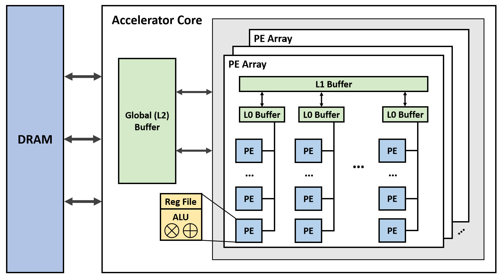
• Parallelism. Parallelism is about allocating the computation workload into the multiple HW processing units and letting these processing units perform the computation simultaneously. For DNN accelerators, the processing units are PEs, and they usually achieve parallelism via unrolling the loop nest of convolutional layers spatially.
• Computation order. Computation order is the temporal order of the dimensions to be performed in the multiple-dimensional computation task. Different computation orders can exploit different data movement patterns and reuse opportunities.
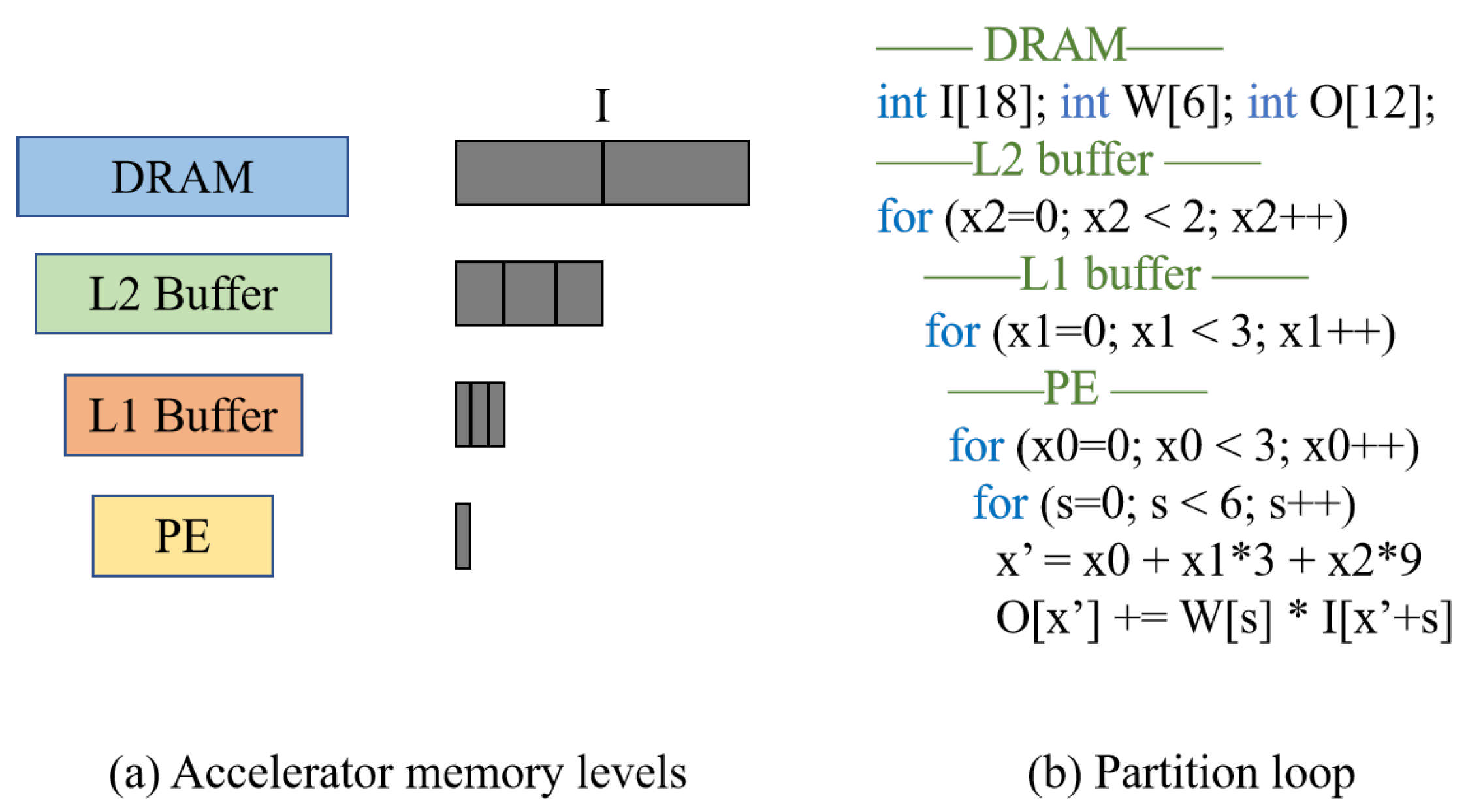
• Partitioning size. As there are many parameters to the DNN application and the buffer size of DNN accelerators is limited, accelerators with a multi-level memory hierarchy will partition these parameters and allocate them into buffers. In this process, the partitioning size will determine the data size of each tensor (input/output/weight) that needs to be present within the accelerator’s buffer.

Although different types of DNNs prefer different dataflow designs, as indicated in Figure 1, existing accelerators either utilize manually designed dataflows [7,9,10] or search the dataflow using conventional optimization algorithms [20,22,23], leading to serious human efforts and suboptimal performance. To tackle this problem, we propose a data-centric method to find the optimal dataflow for DNN layers in seconds without human effort.

3. Our Approach

In this section, we propose Dataflow Code Propagation (DCP) to efficiently search the optimal dataflow for DNN accelerators in a differentiable manner. Towards this goal, we first benchmark the dataflow parameters and DNN layer configurations in Section 3.1. Then, a predictor is trained to predict HW metrics given the dataflow and DNN layer parameters in Section 3.2. Lastly, we search the optimal dataflow for DNN layers by back-propagating the gradients under various objectives such as minimizing latency consumption in Section 3.3. An overview of DCP is shown in Figure 3.

3.1. Benchmarking Dataflow and DNN Layer

We propose an encoding scheme to build the benchmark of the dataflow and the DNN layer where the HW metrics for each pair of dataflow and the DNN layer are evaluated by HW simulation.

Encoding scheme. We encode the dataflow and accompanying DNN layer configurations into coding representations to perform the dataflow optimization efficiently. A detailed example of our coding representation is shown in Figure 4. In our encoding scheme, the configuration of a DNN layer is represented by seven dimensions, which are input row/column ($Y/X$), filter row/column ($R/S$), output/input channels ($K/C$), and an extra dimension (T) to describe the layer type of DNN layers. The row/column of output can be deduced by the input row/column and filter row/column. Overall, we encode a DNN layer into a seven-dimensional code in the order of $K,C,Y,X,R,S,T$, denoted by $x\in {\mathbb{R}}^m$ where $m=7$.

For the coding representation of dataflow, we encode it into a $(3,7,2)$ dimensional code, denoted by $y\in {\mathbb{R}}^n$ where $n=42$. Considering the architecture of the DNN accelerator introduced in Section 2, this “3” refers to the three memory levels of an accelerator. For each memory level, there will be a $(7,2)$ dimensional code to describe the dataflow of one cluster in the corresponding memory level. As demonstrated in Figure 2, a DNN accelerator may have one L2 cluster and several L1/L0 clusters, which contain a memory buffer and corresponding sub-clusters. The “7” in the $(7,2)$ dimensional code of each memory level addresses the seven dimensions. Notably, the first dimension indicates a parallel dimension selected from $K,C,Y,X,R,S$ to be unrolled and perform parallel computation. The remaining six dimensions are obtained by reordering the dimensions of $K,C,Y,X,R,S$ in computation order. Then, the two-dimensional code “2” of each dimension contains a number to index the corresponding dimension and an accompanying number. The accompanying number of the parallel dimension specifies how many PEs will be allocated to perform parallel computation. In contrast, the accompanying number of the remaining six dimensions determines their partitioning size. The size of memory buffers in each sub-clusters is calculated by partitioning size, as the buffers store input, output, and weight tensors. In contrast, the size of these tensors is the linear combination of partitioning sizes.

Hardware metrics. To build the benchmark, we evaluate the HW metrics for each pair of code representations of the dataflow and the DNN layer. However, the above encoding scheme involves a vast search space, making it hard to enumerate all DNN layer dimensions and their corresponding dataflows. For example, the first layer in ResNet101 ($K=64,C=3,Y=224,X=224,R=7,S=7$) can form a dataflow search space with the complexity of $O\left({10}^{36}\right)={(64\times 3\times {224}^2\times 72\times 6!\times 6)}^3$. In practice, we randomly sample $2K$ DNN layers based on all classification models in the torchvision library (version 0.12, including ViT) [38]. For each DNN layer, we sample $2K$ dataflows randomly. We find that such a scale of the dataset is enough to train a good predictor. Then, we evaluate the performance for all sampled dataflows and accompanying DNN layers with a performance simulator [27] or cycle-accurate simulation to form a dataset with the input of our unified coding representation and the output of performance metrics (e.g., latency, energy, etc.).

Collection of data with HW constraints. In the design of realistic DNN accelerators, several constraints should be considered, like the number of PEs contained in the accelerator and the memory size of each buffer. The dataflow encoding scheme introduced above can also address the design constraints of realistic DNN accelerators. The simple one is that the accompanying number of parallels can constrain the number of processing elements in the accelerator and corresponding sub-clusters. We address these constraints of accelerator design by only sampling data satisfying the limitation of these constraints.

3.2. Training Predictor

Unlike previous dataflow designing approaches that require a time-consuming HW simulation process for each model, DCP aims to train a predictor using the benchmark introduced in Section 3.1 to optimize dataflow for all models, as shown in Figure 3.

The training data for the predictor is constructed as described in Section 3.1. We sample a diverse set of DNN layers—including convolutional (CONV), depth-wise convolution (DSCONV), fully connected (FC), pooling (POOL), transposed convolution (TRCONV), group convolution (NGCONV), LSTM, and general matrix multiplication (GEMM) layers—from popular models in the torchvision library. For each layer, $2K$ dataflows are randomly generated, resulting in a comprehensive benchmark that covers a wide range of dataflow and layer configurations. Each (layer, dataflow) pair is evaluated using a hardware simulator to obtain ground-truth metrics such as latency, energy, and power.

Predictor architecture. The neural predictor $\mathcal{F}$ is instantiated by an encoder ${\theta }_e$ and several prediction heads $\left\{{\theta }_i\right\}$ for HW metrics where ${\theta }_i$ indicates the head i-th metric. The encoder is a shallow attention network with a four-layer self-attention layer [39] of hidden size 64. The activation function is Swish [40], and a dropout [41] of $0.1$ is also applied to mitigate the over-fitting of each layer. Note that a linear projection layer is used to project the input to the feature with the size of 512. It is then reshaped to the size of $8\times 64$ where “8” is the token length and “64” is the hidden size. Moreover, each prediction head is instantiated by a single attention layer with an output size of 1. In total, this projector has $0.4M$ parameters and $1M$ FLOPs. Hence, the training cost of the predictor is almost negligible.

Training details. The loss function for training the predictor is generated by three HW metrics (i.e., latency, energy, and power), as shown in Figure 3, considering that both running time and energy consumption are critical for efficient dataflow design. Let $\mathcal{G}$ denote the loss function. The training loss $\mathcal{L}$ is given by

$$\mathcal{L}=\sum _{i=1}^M\mathcal{G}(P_i,R_i)\mathrm{and}{P}_i=\mathcal{F}({\theta }_e,{\theta }_i;[x,y])$$

(1)

where M is the number of HW metrics and $M=3$ in our case. $P_i$ and $R_i$ are the predicted and ground-truth value of the i-th metric. In implementation, $\mathcal{G}$ is log-cosh function as written by $\mathcal{G}(X,Y)=log(cosh(X-Y\left)\right)$.

The predictor is trained on the benchmark in Section 3.1 where $80\%$ and $20\%$ data are used as training and validation sets. In addition, we use the Adam optimizer [42] with parameters $\beta =(0.9,0.999)$ and $ϵ=1\times {10}^{-3}$. The predictor is trained for 50 epochs with initial learning $1\times {10}^{-2}$ and weight decay $1\times {10}^{-7}$.

The regression performance of our neural predictor is shown in Figure 5. It can be seen that the predictor can predict various metrics given dataflow and the DNN layer.

3.3. Dataflow Code Optimization

After training the neural predictor, the dataflow optimization becomes ultra-fast by back-propagating along the direction of target metrics’ gradients. As shown in Figure 3, the predictor will forward an initial dataflow code to obtain predicted performance metrics $P_i$. To minimize (maximize) a metric, we set the target value of the metric as $R_i^{\prime }=P_i-1$ ($R_i^{\prime }=P_i+1$). Then the weight of the predictor will be fixed to perform the back-propagation with respect to the code of dataflow, returning an optimized dataflow after a certain number of iterations. We investigate optimizing dataflow from layer-level, model-level, and multi-objective perspectives.

Layer-level dataflow propagation. The layer-level dataflow propagation aims to search for the optimal dataflow for each layer in a given deep model. Let ${\left\{x_l\right\}}_{l=1}^L$ be the code representations of all layers in the model where L is the number of layers. The layer-level dataflow optimization is derived by gradient descent. For all $l\in \left[L\right]$,

$$y_l^{t+1}=y_l^t-\eta {\displaystyle \frac{\partial \mathcal{G}(\mathcal{F}({\theta }_e^{\mathrm{fix}},{\theta }_i^{\mathrm{fix}};[x_l,y]),R_i^{\prime })}{\partial y}}{|}_{y_l^t}$$

(2)

where $t=0,1\cdots ,T-1$ is the iteration index, $\eta$ is the stepsize, and ${\theta }_e^{\mathrm{fix}}$ and ${\theta }_i^{\mathrm{fix}}$ represent fixed encoder and prediction head of i-th metric, respectively. Note that Equation (2) cannot guarantee that the searched dataflow satisfies the HW constraints, such as the integer requirement of memory. Hence, two modifications are adopted. Firstly, we round the searched dataflow every $T_{int}$ iteration to obtain dataflow parameters with the integer. Secondly, a min-max clip strategy is used to ensure that the dataflow parameters do not exceed the limit of the HW resource constraints.

Model-level dataflow propagation. Although the layer-level dataflow propagation is optimal, it can only be implemented when dataflow is configurable in a HW accelerator. To alleviate this limitation, we also perform model-level dataflow propagation by accumulating the propagation gradient of all layers within the target DNN model:

$$y^{t+1}=y^t-\eta \sum _{l=1}^L{\displaystyle \frac{\partial \mathcal{G}(\mathcal{F}({\theta }_e^{\mathrm{fix}},{\theta }_i^{\mathrm{fix}};[x_l,y]),R_i^{\prime })}{\partial y}}{|}_{y^t}.$$

(3)

The summation means that the layer with a larger number would affect the dataflow update more than the smaller ones. By Equation (3), DCP can search for the best dataflow that is optimized for all layers within a DNN model simultaneously.

Multiple objective propagation. In HW design, we often need to have a trade-off between latency and energy consumption. To this end, we also use multiple objective propagations to search the dataflow, which can be expressed by the following:

$$y_l^{t+1}=y_l^t-\eta \sum _{i=1}^M{\lambda }_i{\displaystyle \frac{\partial \mathcal{G}(\mathcal{F}({\theta }_e^{\mathrm{fix}},{\theta }_i^{\mathrm{fix}};[x_l,y]),R_i^{\prime })}{\partial y}}{|}_{y_l^t}.$$

(4)

where ${\sum }_{i=1}^M{\lambda }_i=1$ uses the weighted average of the gradients of target metrics to perform the back-propagation. Since DCP is fast enough, we can obtain optimal ${\left\{{\lambda }_i\right\}}_{i=1}^M$ by grid search. The summation of gradients in Equation (4) helps find dataflow configuration that can trade off multiple HW metrics better.

4. Experiments

In this section, we first present our experiment settings in Section 4.1. Then, we evaluate our proposed DCP technique in dataflow customization from the perspective of per-layer optimization in Section 4.2, per-model optimization in Section 4.3, and multi-objectives optimization in Section 4.4. Lastly, optimization for unseen HW settings are also performed to show the generalization of DCP in Section 4.5. Besides the aforementioned experiment, an investigation of the optimization for a realistic HW platform is shown in Appendix B.

4.1. Experiment Settings

We consider three representative DNN models with different topology architectures and complexity, i.e., MobileNet-V2 [16], ResNet101 [14], and Vision Transformer (ViT) [15]. The hardware configuration used in our experiments is explicitly specified to match the Edge platform settings described in GAMMA [21], featuring 168 processing elements (PEs), 108 KB of on-chip memory, and a clock frequency of 90 MHz. We evaluate the following optimization methods as the baseline: (i) Random Search: The random search samples the design points randomly and keeps the best solutions. (ii) Genetic Algorithms (GAs): In this baseline, we consider a general GA [43] and GAMMA [21], a specifically designed GA for optimizing the dataflow. (iii) Nevergrad: The rest of our baseline methods are implemented in the optimization algorithm platform Nevergrad [44], including Particle Swarm Optimization (PSO) [45], Passive Portfolio [46], (1 + 1) Evolution Strategy (OnePlusOne) [47], Covariance Matrix Adaptation-ES (CMA) [48], Differential Evolution (DE) [49], and Test-based Population-Size Adaptation (TBPSA) [50].

4.2. Per-Layer Dataflow Optimization

We first perform the per-layer dataflow optimization to evaluate DCP’s performance in searching for the optimal dataflow for each DNN layer within a model and guide the dataflow design of reconfigurable accelerators. In per-layer optimization, DCP and the baseline methods search the optimized dataflow for every layer within a DNN model. All optimization methods in our evaluation are performed multiple times with different objectives (e.g., EDP, latency, and energy), and the detailed performance is summarized in

Table 1. Performance of optimized dataflow for different optimization methods on several DNN models. Each method is performed multiple times with different optimization objectives.

Method	MobileNet-V2 [16]			ResNet101 [14]			ViT [15]			Time Cost
	EDP (Cycles × nJ)	Latency (Cycles)	Energy (nJ)	EDP (Cycles × nJ)	Latency (Cycles)	Energy (nJ)	EDP (Cycles × nJ)	Latency (Cycles)	Energy (nJ)
PSO [45]	$2.14\times {10}^{10}$	$1.72\times {10}^7$	$2.20\times {10}^5$	$5.05\times {10}^{11}$	$4.79\times {10}^7$	$5.90\times {10}^5$	$1.72\times {10}^{13}$	$1.58\times {10}^8$	$8.52\times {10}^5$	4945 s
Portfolio [46]	$1.75\times {10}^{10}$	$1.64\times {10}^7$	$2.16\times {10}^5$	$1.78\times {10}^{11}$	$1.51\times {10}^7$	$5.45\times {10}^5$	$2.75\times {10}^{12}$	$5.50\times {10}^6$	$6.38\times {10}^5$	6010 s
OnePlusOne [47]	$4.44\times {10}^{10}$	$2.14\times {10}^7$	$2.37\times {10}^5$	$4.11\times {10}^{12}$	$1.41\times {10}^8$	$6.86\times {10}^5$	$2.56\times {10}^{15}$	$3.08\times {10}^8$	$8.86\times {10}^5$	4756 s
CMA [48]	$7.83\times {10}^{11}$	$2.91\times {10}^7$	$2.64\times {10}^5$	$2.77\times {10}^{19}$	$9.22\times {10}^{18}$	$9.04\times {10}^5$	$3.14\times {10}^{12}$	$1.79\times {10}^7$	$1.24\times {10}^6$	7529 s
DE [49]	$1.78\times {10}^{10}$	$1.64\times {10}^7$	$2.11\times {10}^5$	$9.14\times {10}^{10}$	$1.51\times {10}^7$	$5.20\times {10}^5$	$3.09\times {10}^{11}$	$4.79\times {10}^5$	$6.84\times {10}^5$	4882 s
TBPSA [50]	$1.90\times {10}^{10}$	$1.68\times {10}^7$	$2.17\times {10}^5$	$2.90\times {10}^{11}$	$2.49\times {10}^7$	$5.47\times {10}^5$	$4.01\times {10}^{11}$	$8.18\times {10}^6$	$6.35\times {10}^5$	4781 s
pureGA [43]	$3.91\times {10}^{10}$	$2.44\times {10}^7$	$2.20\times {10}^5$	$1.64\times {10}^{12}$	$1.17\times {10}^8$	$6.13\times {10}^5$	$4.08\times {10}^{12}$	$4.64\times {10}^6$	$7.91\times {10}^5$	6662 s
Random [51]	$5.12\times {10}^{10}$	$2.08\times {10}^7$	$2.19\times {10}^5$	$1.70\times {10}^{12}$	$1.16\times {10}^8$	$5.94\times {10}^5$	$5.16\times {10}^{11}$	$3.59\times {10}^6$	$8.30\times {10}^5$	4403 s
GAMMA [21]	$2.11\times {10}^9$	$7.63\times {10}^5$	$1.14\times {10}^5$	$2.31\times {10}^{11}$	$1.19\times {10}^7$	$6.62\times {10}^5$	$9.67\times {10}^9$	$2.95\times {10}^5$	$8.56\times {10}^5$	5253 s
DCP (Ours)	$8.88\times {10}^6$	$9.66\times {10}^4$	$3.51\times {10}^3$	$7.18\times {10}^7$	$4.64\times {10}^5$	$1.01\times {10}^4$	$5.70\times {10}^7$	$1.31\times {10}^5$	$1.72\times {10}^4$	3606 s

. We set $10K$ samples as the searching constraint of baseline methods, as we observed that the baseline methods could converge on most DNN Layers after evaluating $10K$ samples. However, for every selected model, some methods face greater difficulty in finding good solutions within $10K$ trials. This observation also reflects the data efficiency of DCP as our neural predictor is trained on a dataset with $2K$ samples for each DNN layer and does not need to evaluate any more samples in back-propagation. For the optimization performance, DCP outperforms all the baseline methods with several orders of magnitude in various HW metrics of MobileNet-V2, ResNet101, and ViT.

We further compare the time cost of DCP and other baseline methods in searching the optimal dataflow for all evaluation metrics of all three selected DNN models. As baseline methods perform dataflow searching and evaluate it with the cost model simultaneously, the time cost of DCP is inclusive of three parts, which are dataset collection, training predictor, and dataflow search. Although the GPU can accelerate DCP by leveraging the differentiable property of back-propagation, we perform the dataflow search of DCP and other baseline methods on the CPU (i5-12500H) for a fair comparison. From Table 1, we see that our DCP is more efficient than other baseline search algorithms. Note that DCP separates the dataflow searching from the data collection, and the searching can be ultra-fast once the neural predictor is trained. Hence, the advantage in the time cost of DCP can be enlarged when more models and HW metrics are evaluated.

Layer-Wise Performance Analysis and Discussion

To provide deeper insight into how DCP achieves its superior per-layer performance, we refer to the illustrative examples and figures provided in the Appendix A (see Figure A1, Figure A2 and Figure A3). These figures demonstrate the fundamental impact of dataflow choices—such as parallelism, computation order, and partitioning size—on memory access patterns and computational efficiency for different types of DNN layers.

For instance, Figure A1 and Figure A2 show how varying the computation order and parallelism in a simple 1D convolution can drastically affect the number of memory accesses and the degree of data reuse. DCP leverages its unified encoding and differentiable optimization to automatically discover such optimal dataflow configurations for each layer, rather than relying on fixed or manually designed strategies. This is particularly beneficial for layers with diverse characteristics. For example, early convolutional layers with large spatial dimensions benefit from maximizing spatial data reuse, while depth-wise or group convolutions require careful balancing of parallelism and buffer allocation due to their lower arithmetic intensity.

The partitioning strategies illustrated in Figure A3 are also automatically tuned by DCP, allowing it to fit data tiles efficiently into the available memory hierarchy, thus reducing expensive off-chip memory accesses. This adaptability is a key reason why DCP consistently outperforms baseline methods, which often apply generic or suboptimal dataflow patterns across all layers.

Moreover, the practical impact of these optimizations is validated by the real hardware experiments shown in Figure A5 (Appendix B), where the DCP-optimized dataflow achieves significant improvements in both latency and energy consumption compared to example dataflows provided by accelerator design frameworks such as Tensorlib. This demonstrates that the benefits of DCP’s layer-wise optimization are not limited to simulation, but also translate to tangible gains on realistic hardware platforms.

In summary, by automatically adapting dataflow parameters to the unique structure and requirements of each layer—guided by a learned predictor and a differentiable search process—DCP is able to exploit data reuse, parallelism, and memory hierarchy far more effectively than traditional search- or rule-based approaches. This results in substantial improvements in key hardware metrics (latency, energy, EDP) across a wide range of DNN models and layer types.

4.3. Per-Model Dataflow Optimization

Compared with reconfigurable accelerators that can utilize a better dataflow for each DNN layer, DNN accelerators designed with a fixed dataflow still dominate in existing accelerators which makes it essential to optimize dataflow for the whole DNN model. And unlike prior studies, DCP can search the optimal dataflow for both DNN layers and an entire DNN model. In model dataflow optimization, we search for the optimal dataflow of three well-known DNN models based on three different metrics (e.g., EDP, latency, and energy). We further compare the performance of DCP-searched dataflow with the dataflow of three well-known state-of-the-art DNN accelerators, which are NVDLA [9], Eyeriss [7], ShiDianNao [10], and the dataflow searched by NAAS [29]. NAAS is a co-design algorithm that targets the same HW platform as ours, and it also performs an experiment that only searches the dataflow in its paper. As is shown in

Table 2. Dataflow performance of DCP, NAAS, and a suite of DNN accelerators with fixed dataflow. DCP’s dataflow is searched by model dataflow propagation, and it is fixed for every DNN model.

Method	MobileNet-V2 [16]			ResNet101 [14]			ViT [15]
	EDP (Cycles × nJ)	Latency (Cycles)	Energy (nJ)	EDP (Cycles × nJ)	Latency (Cycles)	Energy (nJ)	EDP (Cycles × nJ)	Latency (Cycles)	Energy (nJ)
NVDLA [9]	$5.51\times {10}^{11}$	$1.46\times {10}^7$	$1.15\times {10}^6$	$5.60\times {10}^{13}$	$1.84\times {10}^8$	$2.94\times {10}^7$	$1.66\times {10}^{16}$	$4.31\times {10}^9$	$4.51\times {10}^7$
Eyeriss [7]	$1.34\times {10}^{12}$	$2.33\times {10}^7$	$1.71\times {10}^6$	$2.28\times {10}^{14}$	$3.92\times {10}^8$	$3.93\times {10}^7$	$1.96\times {10}^{15}$	$2.53\times {10}^8$	$5.37\times {10}^7$
ShiDianNao [10]	$2.99\times {10}^{11}$	$5.26\times {10}^6$	$1.85\times {10}^6$	$8.00\times {10}^{13}$	$1.20\times {10}^8$	$4.48\times {10}^7$	$2.40\times {10}^{15}$	$1.73\times {10}^8$	$5.71\times {10}^7$
NAAS [29]	$1.09\times {10}^{10}$	$9.23\times {10}^5$	$3.85\times {10}^5$	$5.56\times {10}^{10}$	$2.67\times {10}^7$	$1.39\times {10}^6$	-	-	-
DCP (Ours)	$6.64\times {10}^8$	$7.12\times {10}^5$	$1.19\times {10}^4$	$5.96\times {10}^9$	$9.96\times {10}^6$	$5.12\times {10}^4$	$6.33\times {10}^9$	$2.12\times {10}^6$	$6.55\times {10}^4$

“-” denotes that the corresponding data are not mentioned in the relevant paper.

, DCP outperforms the DNN accelerators’ best performance in all evaluation metrics. An example of the model dataflow searched for MobileNet-v2 is shown in Figure 4. Mobilenet-v2 widely uses depth-wise layers, and it is more efficient to explore parallelism in dimensions of input/output channels [52] that correspond to the optimized dataflow by our DCP. Moreover, compared to the dataflow of NVDLA, which only explores parallelism and data reuse in input/output channels, DCP caches more data in dimensions of input row/column. This helps reduce the data movement between the DRAM and the accelerator’s buffer, which can further minimize runtime and energy consumption.

4.4. Optimizing Dataflow for Multiple Objectives

Unlike the other baseline methods, DCP can optimize the dataflow for both single and multiple objectives as introduced in Section 3.3. In the following experiments, we optimize three metrics in both single-objective and multiple-objective optimization with the pairwise combination of the three metrics. The selected three objective HW metrics are latency, energy, and EDP, and the detailed experimental data are summarized in

Table 3. DCP’s performance of dataflow optimized for single and multiple objectives. Multi-objective optimization includes the pairwise combination of all objectives in single-objective optimization.

Target		Single Objective			Multiple Objective
		Latency	Energy	EDP	Latency + Energy	Latency + EDP	Energy + EDP
MobileNet-V2 [16]	Latency (cycles)	$9.66\times {10}^4$	$3.91\times {10}^5$	$9.83\times {10}^4$	$1.04\times {10}^5$	$1.10\times {10}^5$	$2.21\times {10}^5$
	Energy (nJ)	$5.49\times {10}^3$	$3.51\times {10}^3$	$4.69\times {10}^3$	$4.85\times {10}^3$	$4.75\times {10}^3$	$3.88\times {10}^3$
	EDP (cycles × nJ)	$1.02\times {10}^7$	$2.77\times {10}^7$	$8.88\times {10}^6$	$1.05\times {10}^7$	$1.11\times {10}^7$	$1.92\times {10}^7$
ResNet101 [14]	Latency (cycles)	$4.64\times {10}^5$	$2.20\times {10}^6$	$5.01\times {10}^5$	$5.29\times {10}^5$	$5.28\times {10}^5$	$1.31\times {10}^6$
	Energy (nJ)	$1.76\times {10}^4$	$1.01\times {10}^4$	$1.41\times {10}^4$	$1.45\times {10}^4$	$1.41\times {10}^4$	$1.08\times {10}^4$
	EDP (cycles × nJ)	$7.88\times {10}^7$	$3.00\times {10}^8$	$7.18\times {10}^7$	$8.26\times {10}^7$	$8.16\times {10}^7$	$1.94\times {10}^8$
ViT [15]	Latency (cycles)	$1.31\times {10}^5$	$8.76\times {10}^5$	$1.39\times {10}^5$	$1.76\times {10}^5$	$1.73\times {10}^5$	$1.88\times {10}^5$
	Energy (nJ)	$2.80\times {10}^4$	$1.72\times {10}^4$	$1.88\times {10}^4$	$2.07\times {10}^4$	$2.18\times {10}^4$	$1.99\times {10}^4$
	EDP (cycles × nJ)	$7.28\times {10}^7$	$3.39\times {10}^8$	$5.70\times {10}^7$	$8.24\times {10}^7$	$8.67\times {10}^7$	$8.59\times {10}^7$

. As shown in Table 3, although optimizing dataflow for multiple objectives cannot achieve the best performance in corresponding metrics compared with single-objective optimization, it can achieve comparable performance in multiple metrics simultaneously. For example, compared with optimizing dataflow only for energy, optimizing dataflow for both energy and EDP can significantly improve the performance of latency and EDP while still having a comparable energy consumption.

It is important to note that the multi-objective optimization results show that combining objectives leads to slightly worse performance compared to single-objective optimization. This is expected and can be explained by several factors:

(1) Trade-off Nature of Objectives: Latency and energy are inherently competing objectives. Optimizing for one often degrades the other, making it challenging to find configurations that excel at both simultaneously. In practice, the hardware configurations that minimize latency may require more parallelism or buffer usage, which can increase energy consumption, and vice versa.

(2) Gradient Conflict: During back-propagation, the gradients from different objectives may point in opposing directions, leading to suboptimal updates that do not fully optimize either objective. This gradient conflict is a well-known challenge in multi-objective optimization, where the optimizer must balance competing directions in the parameter space.

(3) Pareto Frontier Limitations: The multi-objective approach finds solutions on the Pareto frontier, which represents the best possible trade-offs, but these solutions are inherently compromises between competing objectives. For example, for MobileNet-V2, the latency + energy combination achieves $1.04\times {10}^5$ cycles versus $9.66\times {10}^4$ for single-objective latency optimization, representing a 7.7% degradation but providing better energy efficiency. Similar patterns are observed for other models and objective combinations, where the combined optimization prioritizes balanced trade-offs over pure optimization of a single metric.

(4) Objective Weighting and Sensitivity: The choice of weights (${\lambda }_i$) in the multi-objective loss function can significantly affect the optimization trajectory. If the objectives have different scales or sensitivities, the optimization may be biased toward one metric, making it difficult to achieve a truly balanced solution without careful tuning or normalization.

In summary, the observed performance gap between single- and multi-objective optimization is a natural consequence of the underlying trade-offs and optimization dynamics. While multi-objective optimization provides more balanced solutions, it is fundamentally constrained by the conflicting nature of hardware metrics and the challenges of navigating a high-dimensional, non-convex search space.

4.5. Optimizing Dataflow for Unseen HW Settings

In this experiment, we execute DCP in zero-shot or few-shot unseen HW settings to evaluate the generalization of DCP. Initially, the neural predictor is trained with a dataset that randomly sampled 2K dataflows for each DNN layer under the HW setting of Eyeriss chip [7], which is 168 PEs and 108KB on-chip memory. In zero-shot settings, we execute DCP with this original neural predictor. Then in the few-shot settings, we fine-tune the neural predictor with a dataset that randomly sampled 200 dataflows for DNN layers within the previous dataset under the corresponding unseen HW settings. The selected unseen HW settings share the same on-chip memory as the Eyeriss chip but with different PEs. As demonstrated in Figure 6, DCP in the zero-shot setting outperforms GAMMA (best baseline method performed in Section 4.2) in MobileNet-V2, ResNet101, and ViT, while GAMMA needs to evaluate 10K samples from scratch for each DNN layer. Then for the few-shot setting, DCP can search the better dataflow after fine-tuning the neural predictor.

Limitations and challenges. While DCP demonstrates strong generalization in both zero-shot and few-shot settings, there are important limitations to consider. The approach is most effective when the unseen hardware configurations are similar to those represented in the training data, such as moderate changes in the number of processing elements (PEs) or buffer sizes. However, when the target hardware differs substantially from the training distribution—such as drastic changes in memory hierarchy, the introduction of new types of compute units, or highly irregular resource constraints—the predictor may not accurately capture the new performance landscape. In these cases, the optimization may yield suboptimal or even invalid dataflow configurations, and additional data collection and retraining (or architectural adaptation) may be required. Furthermore, the current encoding scheme assumes a certain regularity in hardware structure; highly heterogeneous or non-standard architectures may require new encoding strategies or more flexible predictor models. We encourage future works to explore more robust generalization techniques and adaptive encoding methods to address these challenging scenarios.

5. Conclusions

In this paper, we present a differentiable back-propagation approach, DCP, to automatically search the optimal dataflow for DNN accelerators. Dataflow is crucial for designing a DNN accelerator, but identifying the best dataflow is challenging due to its massive design space. Therefore, we propose an encoding scheme to project the dataflow and DNN layer configurations into a unified coding representation and build a comprehensive benchmark. DCP can optimize dataflow for single/multiple layers and various optimization objectives. Our results show that DCP outperforms the existing dataflow optimization methods in both optimization performance and time cost. DCP also outperforms prior studies in zero-shot or few-shot manners without time-consuming simulations, while prior studies need to re-run the simulations from scratch for every search.

In the Appendix A, we provide more details of dataflow and an experiment about performing DCP in a realistic HW platform in Appendix A and Appendix B, respectively.

References

1. He, K.; Chen, X.; Xie, S.; Li, Y.; Dollár, P.; Girshick, R. Masked autoencoders are scalable vision learners. arXiv 2021, arXiv:2111.06377. [Google Scholar]
2. Al-Qizwini, M.; Barjasteh, I.; Al-Qassab, H.; Radha, H. Deep learning algorithm for autonomous driving using GoogLeNet. In Proceedings of the 2017 IEEE Intelligent Vehicles Symposium (IV), Los Angeles, CA, USA, 11–14 June 2017; pp. 89–96. [Google Scholar]
3. Jumper, J.; Evans, R.; Pritzel, A.; Green, T.; Figurnov, M.; Ronneberger, O.; Tunyasuvunakool, K.; Bates, R.; Žídek, A.; Potapenko, A.; et al. Highly accurate protein structure prediction with AlphaFold. Nature 2021, 596, 583–589. [Google Scholar] [CrossRef]
4. Tan, M.; Chen, B.; Pang, R.; Vasudevan, V.; Sandler, M.; Howard, A.; Le, Q.V. MnasNet: Platform-Aware Neural Architecture Search for Mobile. In Proceedings of the 2019 IEEE/CVF Conference on Computer Vision and Pattern Recognition (CVPR), Long Beach, CA, USA, 16–20 June 2019; pp. 2815–2823. [Google Scholar]
5. Ma, N.; Zhang, X.; Zheng, H.T.; Sun, J. ShuffleNet V2: Practical Guidelines for Efficient CNN Architecture Design. In Proceedings of the Computer Vision–ECCV, Munich, Germany, 8–14 September 2018; Ferrari, V., Hebert, M., Sminchisescu, C., Weiss, Y., Eds.; pp. 122–138. [Google Scholar]
6. Iandola, F.N.; Han, S.; Moskewicz, M.W.; Ashraf, K.; Dally, W.J.; Keutzer, K. SqueezeNet: AlexNet-level accuracy with 50x fewer parameters and <0.5MB model size. In Proceedings of the 2017 International Conference on Learning Representations (ICLR), Toulon, France, 24–26 April 2017. [Google Scholar]
7. Chen, Y.H.; Krishna, T.; Emer, J.S.; Sze, V. Eyeriss: An Energy-Efficient Reconfigurable Accelerator for Deep Convolutional Neural Networks. IEEE J.-Solid-State Circuits 2017, 52, 127–138. [Google Scholar] [CrossRef]
8. Chen, Y.H.; Yang, T.J.; Emer, J.; Sze, V. Eyeriss v2: A Flexible Accelerator for Emerging Deep Neural Networks on Mobile Devices. IEEE J. Emerg. Sel. Top. Circuits Syst. 2019, 9, 292–308. [Google Scholar] [CrossRef]
9. NVDLA Deep Learning Accelerator. Available online: http://nvdla.org/primer.html (accessed on 15 March 2018).
10. Du, Z.; Fasthuber, R.; Chen, T.; Ienne, P.; Li, L.; Luo, T.; Feng, X.; Chen, Y.; Temam, O. ShiDianNao: Shifting vision processing closer to the sensor. In Proceedings of the 2015 ACM/IEEE 42nd Annual International Symposium on Computer Architecture (ISCA), Portland, OR, USA, 13–17 June 2015; pp. 92–104. [Google Scholar]
11. Jouppi, N.P.; Young, C.; Patil, N.; Patterson, D.; Agrawal, G.; Bajwa, R.; Bates, S.; Bhatia, S.; Boden, N.; Borchers, A.; et al. In-datacenter performance analysis of a tensor processing unit. In Proceedings of the 2017 ACM/IEEE 44th Annual International Symposium on Computer Architecture (ISCA), Toronto, ON, Canada, 24–28 June 2017; pp. 1–12. [Google Scholar]
12. Parashar, A.; Rhu, M.; Mukkara, A.; Puglielli, A.; Venkatesan, R.; Khailany, B.; Emer, J.; Keckler, S.W.; Dally, W.J. SCNN: An accelerator for compressed-sparse convolutional neural networks. In Proceedings of the 2017 ACM/IEEE 44th Annual International Symposium on Computer Architecture (ISCA), Toronto, ON, Canada, 24–28 June 2017; pp. 27–40. [Google Scholar]
13. Akhlaghi, V.; Yazdanbakhsh, A.; Samadi, K.; Gupta, R.K.; Esmaeilzadeh, H. SnaPEA: Predictive Early Activation for Reducing Computation in Deep Convolutional Neural Networks. In Proceedings of the 2018 ACM/IEEE 45th Annual International Symposium on Computer Architecture (ISCA), Los Angeles, CA, USA, 1–6 June 2018; pp. 662–673. [Google Scholar]
14. He, K.; Zhang, X.; Ren, S.; Sun, J. Deep Residual Learning for Image Recognition. In Proceedings of the 2016 IEEE Conference on Computer Vision and Pattern Recognition (CVPR), Las Vegas, NV, USA, 27–30 June 2016; pp. 770–778. [Google Scholar]
15. Dosovitskiy, A.; Beyer, L.; Kolesnikov, A.; Weissenborn, D.; Zhai, X.; Unterthiner, T.; Dehghani, M.; Minderer, M.; Heigold, G.; Gelly, S.; et al. An Image is Worth 16 × 16 Words: Transformers for Image Recognition at Scale. arXiv 2020, arXiv:2010.11929. [Google Scholar]
16. Sandler, M.; Howard, A.; Zhu, M.; Zhmoginov, A.; Chen, L.C. MobileNetV2: Inverted Residuals and Linear Bottlenecks. In Proceedings of the 2018 IEEE/CVF Conference on Computer Vision and Pattern Recognition, Salt Lake City, UT, USA, 18–23 June 2018; pp. 4510–4520. [Google Scholar]
17. Kwon, H.; Samajdar, A.; Krishna, T. MAERI: Enabling Flexible Dataflow Mapping over DNN Accelerators via Reconfigurable Interconnects. SIGPLAN Not. 2018, 53, 461–475. [Google Scholar] [CrossRef]
18. Yazdanbakhsh, A.; Angermüller, C.; Akin, B.; Zhou, Y.; Jones, A.; Hashemi, M.; Swersky, K.; Chatterjee, S.; Narayanaswami, R.; Laudon, J. Apollo: Transferable Architecture Exploration. arXiv 2021, arXiv:2102.01723. [Google Scholar]
19. Kao, S.C.; Jeong, G.; Krishna, T. ConfuciuX: Autonomous Hardware Resource Assignment for DNN Accelerators using Reinforcement Learning. In Proceedings of the 2020 53rd Annual IEEE/ACM International Symposium on Microarchitecture (MICRO), Athens, Greece, 17–21 October 2020; pp. 622–636. [Google Scholar]
20. Wang, J.; Guo, L.; Cong, J. AutoSA: A Polyhedral Compiler for High-Performance Systolic Arrays on FPGA. In Proceedings of the The 2021 ACM/SIGDA International Symposium on Field-Programmable Gate Arrays, Virtual Event, USA, 28 February–2 March 2021; FPGA’21. pp. 93–104. [Google Scholar]
21. Kao, S.C.; Krishna, T. GAMMA: Automating the HW Mapping of DNN Models on Accelerators via Genetic Algorithm. In Proceedings of the 39th International Conference on Computer-Aided Design, New York, NY, USA, 2–6 November 2020. ICCAD’20. [Google Scholar]
22. Parashar, A.; Raina, P.; Shao, Y.S.; Chen, Y.H.; Ying, V.A.; Mukkara, A.; Venkatesan, R.; Khailany, B.; Keckler, S.W.; Emer, J. Timeloop: A Systematic Approach to DNN Accelerator Evaluation. In Proceedings of the 2019 IEEE International Symposium on Performance Analysis of Systems and Software (ISPASS), Madison, WI, USA, 24–26 March 2019; pp. 304–315. [Google Scholar]
23. Yang, X.; Gao, M.; Liu, Q.; Setter, J.; Pu, J.; Nayak, A.; Bell, S.; Cao, K.; Ha, H.; Raina, P.; et al. Interstellar: Using Halide’s Scheduling Language to Analyze DNN Accelerators. In Proceedings of the Twenty-Fifth International Conference on Architectural Support for Programming Languages and Operating Systems, Lausanne, Switzerland, 16–20 March 2020; Association for Computing Machinery: New York, NY, USA, 2020; pp. 369–383. [Google Scholar]
24. Kawamoto, R.; Taichi, M.; Kabuto, M.; Watanabe, D.; Izumi, S.; Yoshimoto, M.; Kawaguchi, H. A 1.15-TOPS 6.57-TOPS/W DNN Processor for Multi-Scale Object Detection. In Proceedings of the 2020 2nd IEEE International Conference on Artificial Intelligence Circuits and Systems (AICAS), Genova, Italy, 31 August–2 September 2020; pp. 203–207. [Google Scholar]
25. Yamada, Y.; Sano, T.; Tanabe, Y.; Ishigaki, Y.; Hosoda, S.; Hyuga, F.; Moriya, A.; Hada, R.; Masuda, A.; Uchiyama, M.; et al. 7.2 A 20.5TOPS and 217.3GOPS/mm2 Multicore SoC with DNN Accelerator and Image Signal Processor Complying with ISO26262 for Automotive Applications. In Proceedings of the 2019 IEEE International Solid- State Circuits Conference-(ISSCC), San Francisco, CA, USA, 17–21 February 2019; pp. 132–134. [Google Scholar]
26. Kawamoto, R.; Taichi, M.; Kabuto, M.; Watanabe, D.; Izumi, S.; Yoshimoto, M.; Kawaguchi, H.; Matsukawa, G.; Goto, T.; Kojima, M. A 1.15-TOPS 6.57-TOPS/W Neural Network Processor for Multi-Scale Object Detection with Reduced Convolutional Operations. IEEE J. Sel. Top. Signal Process. 2020, 14, 634–645. [Google Scholar] [CrossRef]
27. Kwon, H.; Chatarasi, P.; Pellauer, M.; Parashar, A.; Sarkar, V.; Krishna, T. Understanding Reuse, Performance, and Hardware Cost of DNN Dataflow: A Data-Centric Approach. In Proceedings of the 52nd Annual IEEE/ACM International Symposium on Microarchitecture, Columbus, OH, USA, 12–16 October 2019; MICRO ’52. pp. 754–768. [Google Scholar]
28. Fasfous, N.; Vemparala, M.R.; Frickenstein, A.; Valpreda, E.; Salihu, D.; Höfer, J.; Singh, A.; Nagaraja, N.S.; Voegel, H.J.; Vu Doan, N.A.; et al. AnaCoNGA: Analytical HW-CNN Co-Design Using Nested Genetic Algorithms. In Proceedings of the 2022 Design, Automation & Test in Europe Conference & Exhibition (DATE), Antwerp, Belgium, 14–23 March 2022; pp. 238–243. [Google Scholar]
29. Lin, Y.; Yang, M.; Han, S. NAAS: Neural Accelerator Architecture Search. In Proceedings of the 2021 58th ACM/IEEE Design Automation Conference (DAC), San Francisco, CA, USA, 5–9 December 2021; pp. 1051–1056. [Google Scholar]
30. Fasfous, N.; Vemparala, M.R.; Frickenstein, A.; Valpreda, E.; Salihu, D.; Höfer, J.; Singh, A.; Nagaraja, N.S.; Voegel, H.J.; Vu Doan, N.A.; et al. Auto-NBA: Efficient and Effective Search Over the Joint Space of Networks, Bitwidths, and Accelerators. In Proceedings of the 2021 38th International Conference on Machine Learning (ICML), Virtual Event, 18–24 July 2021; pp. 238–243. [Google Scholar]
31. Choi, K.; Hong, D.; Yoon, H.; Yu, J.; Kim, Y.; Lee, J. DANCE: Differentiable Accelerator/Network Co-Exploration. In Proceedings of the 2021 58th ACM/IEEE Design Automation Conference (DAC), San Francisco, CA, USA, 5–9 December 2021; pp. 337–342. [Google Scholar]
32. Li, Y.; Hao, C.; Zhang, X.; Liu, X.; Chen, Y.; Xiong, J.; Hwu, W.m.; Chen, D. EDD: Efficient Differentiable DNN Architecture and Implementation Co-search for Embedded AI Solutions. In Proceedings of the 2020 57th ACM/IEEE Design Automation Conference (DAC), San Francisco, CA, USA, 20–24 July 2020; pp. 1–6. [Google Scholar]
33. Zhou, Y.; Dong, X.; Meng, T.; Tan, M.; Akin, B.; Peng, D.; Yazdanbakhsh, A.; Huang, D.; Narayanaswami, R.; Laudon, J. Towards the Co-design of Neural Networks and Accelerators. Proc. Mach. Learn. Syst. 2022, 4, 141–152. [Google Scholar]
34. Abdelfattah, M.S.; Dudziak, L.; Chau, T.; Lee, R.; Kim, H.; Lane, N.D. Best of Both Worlds: AutoML Codesign of a CNN and its Hardware Accelerator. In Proceedings of the 2020 57th ACM/IEEE Design Automation Conference (DAC), San Francisco, CA, USA, 20–24 July 2020; pp. 1–6. [Google Scholar]
35. Yang, L.; Yan, Z.; Li, M.; Kwon, H.; Lai, L.; Krishna, T.; Chandra, V.; Jiang, W.; Shi, Y. Co-Exploration of Neural Architectures and Heterogeneous ASIC Accelerator Designs Targeting Multiple Tasks. In Proceedings of the 2020 57th ACM/IEEE Design Automation Conference (DAC), San Francisco, CA, USA, 20–24 July 2020; pp. 1–6. [Google Scholar]
36. Ding, M.; Huo, Y.; Lu, H.; Yang, L.; Wang, Z.; Lu, Z.; Wang, J.; Luo, P. Learning versatile neural architectures by propagating network codes. arXiv 2021, arXiv:2103.13253. [Google Scholar]
37. Horowitz, M. 1.1 Computing’s energy problem (and what we can do about it). In Proceedings of the 2014 IEEE International Solid-State Circuits Conference Digest of Technical Papers (ISSCC), San Francisco, CA, USA, 9–13 February 2014; pp. 10–14. [Google Scholar]
38. TORCHVISION. Available online: https://github.com/pytorch/vision/tree/v0.12.0-rc1 (accessed on 15 June 2022).
39. Subakan, C.; Ravanelli, M.; Cornell, S.; Bronzi, M.; Zhong, J. Attention Is All You Need In Speech Separation. In Proceedings of the ICASSP 2021-2021 IEEE International Conference on Acoustics, Speech and Signal Processing (ICASSP), Toronto, ON, Canada, 6–11 June 2021; pp. 21–25. [Google Scholar]
40. Ramachandran, P.; Zoph, B.; Le, Q.V. Searching for Activation Functions. arXiv 2017, arXiv:1710.05941. [Google Scholar]
41. Srivastava, N.; Hinton, G.; Krizhevsky, A.; Sutskever, I.; Salakhutdinov, R. Dropout: A Simple Way to Prevent Neural Networks from Overfitting. J. Mach. Learn. Res. 2014, 15, 1929–1958. [Google Scholar]
42. Kingma, D.P.; Ba, J. Adam: A Method for Stochastic Optimization. arXiv 2015, arXiv:1412.6980. [Google Scholar]
43. Goldberg, D.E. Genetic Algorithms in Search, Optimization and Machine Learning, 1st ed.; Addison-Wesley Longman Publishing Co., Inc.: Reading, MA, USA, 1989. [Google Scholar]
44. Rapin, J.; Teytaud, O. Nevergrad-A Gradient-Free Optimization Platform. Available online: https://GitHub.com/FacebookResearch/Nevergrad (accessed on 15 December 2018).
45. Marini, F.; Walczak, B. Particle swarm optimization (PSO). A tutorial. Chemom. Intell. Lab. Syst. 2015, 149, 153–165. [Google Scholar] [CrossRef]
46. McMillan, C.; Grechanik, M.; Poshyvanyk, D.; Xie, Q.; Fu, C. Portfolio: Finding Relevant Functions and Their Usage. In Proceedings of the 33rd International Conference on Software Engineering, Honolulu, HI, USA, 21–28 May 2011; ICSE’11. pp. 111–120. [Google Scholar]
47. Igel, C.; Suttorp, T.; Hansen, N. A Computational Efficient Covariance Matrix Update and a (1+1)-CMA for Evolution Strategies. In Proceedings of the 8th Annual Conference on Genetic and Evolutionary Computation, Seattle, WA, USA, 8–12 July 2006; GECCO’06. pp. 453–460. [Google Scholar]
48. Hansen, N.; Niederberger, A.S.P.; Guzzella, L.; Koumoutsakos, P. A Method for Handling Uncertainty in Evolutionary Optimization With an Application to Feedback Control of Combustion. IEEE Trans. Evol. Comput. 2009, 13, 180–197. [Google Scholar] [CrossRef]
49. Vodopija, A.; Tušar, T.; Filipič, B. Comparing Black-Box Differential Evolution and Classic Differential Evolution. In Proceedings of the Genetic and Evolutionary Computation Conference Companion, Kyoto, Japan, 15–19 July 2018; GECCO’18. pp. 1537–1544. [Google Scholar]
50. Poláková, R.; Tvrdík, J.; Bujok, P. Adaptation of population size according to current population diversity in differential evolution. In Proceedings of the 2017 IEEE Symposium Series on Computational Intelligence (SSCI), Honolulu, HI, USA, 27 November–1 December 2017; pp. 1–8. [Google Scholar]
51. Bergstra, J.; Bengio, Y. Random Search for Hyper-Parameter Optimization. J. Mach. Learn. Res. 2012, 13, 281–305. [Google Scholar]
52. Li, G.; Zhang, J.; Zhang, M.; Wu, R.; Cao, X.; Liu, W. Efficient depthwise separable convolution accelerator for classification and UAV object detection. Neurocomputing 2022, 490, 1–16. [Google Scholar] [CrossRef]
53. Jia, L.; Luo, Z.; Lu, L.; Liang, Y. TensorLib: A Spatial Accelerator Generation Framework for Tensor Algebra. In Proceedings of the 2021 58th ACM/IEEE Design Automation Conference (DAC), San Francisco, CA, USA, 5–9 December 2021; pp. 865–870. [Google Scholar]
Figure 1. Dataflow comparisons and explanations. (a) We compare the energy-delay-product (EDP, lower is better) between NVDLA, Eyeriss, ShiDianNao, and our DCP. We see that DCP can achieve the best efficiency for all three visual models. (b) We visualize and compare the dataflow of ours and Eyeriss using the first layer of ResNet101. The layer dimensions have been tiled based on the partitioning size of dataflow. The red color labels the tiles to perform parallel computation, and the orange arrow implies the computation order, where K , C , R , S , Y , X , Y , X represent output/input channels, filter row/column, input row/column, and output row/column, respectively. Our learned dataflow costs only 18.9% read/writes compared to Eyeriss by (i) using a smaller kernel tiled size ( 4 × 4 versus 1 × 1 in Eyeriss) and smaller tiled output channels (8 versus 4 in Eyeriss) but a larger one for input ( 3 × 3 versus 7 × 7 in Eyeriss) and (ii) a different computation order of dimensions.
Electronics 14 03085 g001
Figure 2. Example of DNN accelerator. An abstract DNN accelerator architecture that contains a hierarchical memory system and PE arrays. This abstract DNN accelerator architecture is also used in many DNN accelerators [7,11,12,13].
Electronics 14 03085 g002
Figure 3. An overview of our Dataflow Code Propagation (DCP). DCP first builds a benchmark of dataflow and DNN layer and then trains a predictor to predict various HW metrics. Finally, we back-propagate the gradients of the fixed neural predictor to efficiently update the dataflow code towards the optimization objective (lower predicted metrics), conditioned on the layer code.
Electronics 14 03085 g003
Figure 4. Coding representations of dataflow and DNN layers. DNN layer code is a seven-dimensional code that describes the DNN layer in the dimensions of K , C , Y , X , R , S , T . We use a dataflow optimized for MobileNet-v2 as an example. The dataflow code describes the three memory levels of the accelerator. The L1 dataflow code is an example. The first line is the index of seven dimensions, and the second line is their accompanying numbers. These seven dimensions contain six dimensions in the DNN layer code, except T in computation order and a parallel dimension selected from them to perform parallel computation. The accompanying number of the parallel dimension specifies the number of PEs allocated in one cluster of L1 memory. In contrast, the partitioning size is the accompanying number of the remaining six dimensions.
Electronics 14 03085 g004
Figure 5. Regression performance of the neural predictor for the HW metrics of latency, energy, and power, respectively.
Electronics 14 03085 g005
Figure 6. Performance (EDP) on three DNN models of the dataflow searched on different HW settings. Three approaches are compared in this figure. “DCP zero-shot” denotes the dataflow searched with the neural predictor only trained on the 168 PEs, and “DCP few-shot” denotes the dataflow searched with the neural predictor tuned with 0.1 × samples of corresponding PEs. “GAMMA” denotes the dataflow searched by the specifically designed GA algorithm, GAMMA [21].
Electronics 14 03085 g006