Abstract
The digital transformation of manufacturing through OT, IoT, and AI integration has created extensive networked sensor ecosystems, introducing critical cybersecurity vulnerabilities at IT-OT interfaces. This might particularly challenge the detection component of the NIST cybersecurity framework. To address this concern, the authors designed a diverse machine learning-based intrusion detection system framework for industrial control systems (DICS). DICS implements a sophisticated dual-module architecture. The screening analysis module initially categorizes network traffic as either unidentifiable or recognized packets, while the classification analysis module subsequently determines specific attack types for identifiable traffic. When unrecognized zero-day attack traffic accumulates in a buffer and reaches a predetermined threshold, the agile training module incorporates these patterns into the system, which enables continuous adaptation. During experimental validation, the authors rigorously assess dataset industrial relevance and strategically divide the datasets into four distinct groups to accurately simulate diverse network traffic patterns characteristic of real industrial environments. Moreover, the authors highlight the system’s alignment with IEC 62443 requirements for industrial control system security. In conclusion, the comprehensive analysis demonstrates that DICS delivers superior detection capabilities for malicious network traffic in industrial settings.
1. Introduction
Enhancing production management efficiency has been a crucial objective in the manufacturing industry. This objective has driven a global industrial transformation, which includes operation technology (OT) for factory equipment management, Internet of Things (IoT), Industry 4.0, and smart manufacturing [,,]. Throughout the development, testing, integration, and operational phases, a series of sensor-related monitoring and control signal data are generated. These data undergo various processes for comprehensive integration, including transmission, storage, and retrieval. The processed data then support analytical optimization across manufacturing operations. The evolution of industrial IoT (IIoT) and Artificial Intelligence of Things (AIoT) necessitates controlled information processing across all operational aspects. Therefore, industrial automation and control systems (IACSs) require robust information security techniques, which are essential for establishing proper security protection.
The information technology (IT) industry has developed various security technologies to ensure data confidentiality, integrity, and availability. Security technologies include watermarking [], public key cryptography [], blockchain technology [], and machine learning detection systems []. Industrial control system security presents unique challenges that extend beyond traditional IT security concerns. This is particularly evident in companies with international operations, where diverse network information flows are essential for monitoring automated production lines and equipment status. Production equipment availability is crucial for minimizing operational disruptions. Companies implement monitoring systems to detect potential equipment anomalies and prevent unexpected production line interruptions. The detection equipment enables system integrators to accurately predict automation equipment performance, thereby enhancing their business reputation. IEC 62443 [] is a security standard designed explicitly for IACSs, which covers diverse industrial sectors, including manufacturing facilities, oil production pipelines, and semiconductor fabrication plants. After that, this standard defines four essential roles within the industrial security ecosystem: product supplier, system integrator, service provider, and asset owner []. IEC 62443 marks a significant evolution beyond traditional vendor-dependent security approaches, with major industry leaders such as Siemens demonstrating commitment through certification attainment [,]. However, the boundary protection mechanisms at the IT-OT convergence points remain particularly vulnerable during information exchange processes, which creates critical security gaps. To the best of our knowledge, existing detection models are predominantly static in nature. Current solutions lack self-evolution capabilities and rely solely on passive and irregular vendor updates, making them inadequate for addressing evolving attack patterns such as zero-day attacks. This challenge directly corresponds to the detection component of the NIST cybersecurity framework [], representing a crucial element in comprehensive security architecture.
To address the vulnerability, the authors propose a diverse ML-based intrusion detection system for industrial control systems (DICS), which comprises three functional modules: the screening analysis module (SAM), the classification analysis module (CAM), and the agile training module (ATM). Firstly, the SAM is used to examine all incoming network traffic in the industrial control environment. Unidentifiable traffic patterns are temporarily stored in a buffer for further learning, while identifiable packets are forwarded to the CAM. The CAM employs random forest and K-nearest neighbor models to classify packets into specific traffic categories. Furthermore, DICS implements ATM to process unidentified traffic patterns stored in the buffer. The learning outcomes are continuously fed back to both the SAM and CAM, enabling progressive enhancement of detection capabilities. Experimental results demonstrate the effectiveness of both detection modules through quantitative evaluation. The selected datasets have been thoroughly validated for their suitability in industrial control security applications. To enhance simulation fidelity, we strategically partitioned the dataset into four distinct experimental groups, which better reflect the diverse network traffic patterns characteristic of specialized industrial control environments. Moreover, the authors explicitly highlight the system’s alignment with IEC 62443 requirements for industrial control system security. Next, the analysis systematically compares system performance metrics before and after implementing the agile training mechanism. According to the experimental outcomes, DICS successfully identifies learned attack patterns and demonstrates improved capability in recognizing previously unidentifiable packets following the implementation of the agile training mechanism.
2. Preliminary
This section introduces the technical components utilized in DICS. The components include Autoencoder, random forest, and KNN, with their architectures and characteristics detailed in Section 2.1, Section 2.2 and Section 2.3.
2.1. Autoencoder
Autoencoder represents an unsupervised learning method []. As illustrated in Figure 1, the architecture consists of three primary components: the input layer, the hidden layer, and the output layer, which form the encoder and decoder structures.
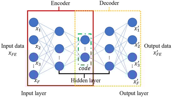
Figure 1.
Architecture of Autoencoder.
The encoder E transforms high-dimensional input data into low-dimensional code, while the decoder D reconstructs high-dimensional data from this code. The transformations are expressed in Equations (1) and (2).
where and denote the activation functions for the encoder and decoder, respectively. The parameters CD, ND, CE, and NE represent the coefficients and neurons in the decoder and encoder architectures. The original feature data xFE and reconstructed feature data each contain F features, with xFE comprising . The code values range between 0 and 1.
The loss function lossAE, as shown in Equation (3), quantifies the difference between x and x′ using mean square error MSE. This loss function exhibits lower values for known (trained) data and higher values for unknown data, enabling the distinction between familiar and unfamiliar patterns.
2.2. Random Forest
Random forest constitutes a supervised learning algorithm and an enhanced variant of the decision tree methodology []. The training process constructs multiple decision trees to establish a random forest structure. As shown in Figure 2, the algorithm builds n decision trees using the training dataset and then performs majority voting on predictions for input data xFE across all trees to determine the final classification outcome.
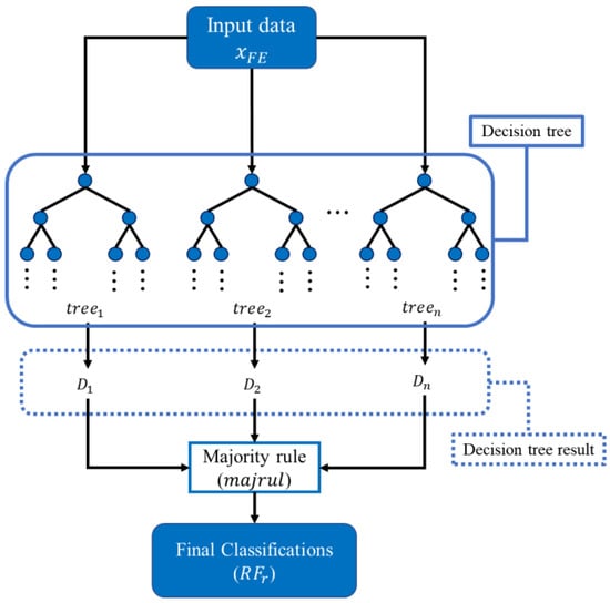
Figure 2.
Architecture of random forest.
As expressed in Equation (4), if a random forest comprises n decision trees, the prediction of the e-th tree for input xFE is denoted as De(xFE), where . Each De(xFE) outputs exclusively from v distinct classes in the training dataset, where and represent the V-th class in cQ. The indicator function I(·) tracks prediction outcomes Dresult, returning 1 when De(xFE) matches the current , or 0 otherwise. The prediction frequencies for each class in cQ are stored in Dresult, and the final random forest prediction RFresult is determined through majority rule majrul by selecting the most frequently predicted class.
2.3. K-Nearest Neighbor (KNN)
K-nearest neighbor functions as a clustering algorithm within supervised machine learning [], which performs classification based on inter-data distances without generating a neural network model. The algorithm constructs a data distribution map using the training dataset T, where yi encompasses two distinct classes represented by yellow triangles and red circles, respectively. As illustrated in Figure 3, the green square denotes the feature vector xFE to be classified, while the spatial distribution is determined by the feature characteristics of each training instance. For a user-specified k value, the algorithm identifies k nearest data points to xFE and assigns the predominant class label among these neighbors, as demonstrated by the enclosed region containing five nearest points when k = 5.
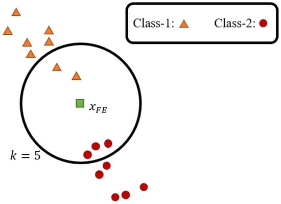
Figure 3.
Architecture of KNN.
As formulated in Equation (5), NK(xFE) represents the class of the K-th nearest neighbor to xFE, where , constrained to the classes present in the training dataset. The training set encompasses v distinct classes denoted as , where indicates the V-th class in cJ. I(·) yields 1 when NK(xFE) matches the currently recorded class, or 0 otherwise. The classification frequencies for each class in cJ are accumulated in Kresult, and the final value of KNNresult prediction is determined through majrul by selecting the most frequently occurring class in Rresult.
3. Proposed Scheme
This section presents various ML-based intrusion detection systems for industrial control systems, simply named DICS. DICS mainly has three modules: the packet screening analysis module (SAM), the packet classification analysis module (CAM), and the agile training module (ATM), as shown in Figure 4. The input packet xFE undergoes preprocessing via normalization [] and standardization []. Next, the preprocessed packet is checked by the SAM and CAM in an orderly manner to determine whether it is the recognized classification or not. If it is not, DICS stores it in a buffer. When the amount reaches the threshold, DICS activates the ATM to update both the SAM and CAM. Details of the SAM, CAM, and ATM are described in Section 3.1, Section 3.2 and Section 3.3, respectively.
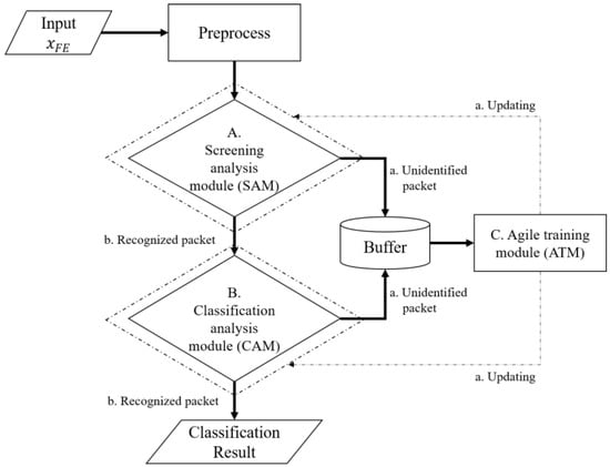
Figure 4.
The framework of DICS.
3.1. Screening Analysis Module (SAM)
The SAM is used as a preliminary detector for checking whether the input packet is known or not, which is based on Autoencoder. First, the features of the preprocessed input xFE undergo dimension reduction via Equation (1) to acquire a low-dimension value code. Then, code is reconstructed through Equation (2) to obtain high-dimension . Later, the SAM computes the difference between xFE and via Equation (3). After that, the SAM is able to perform classification based on the threshold THAE. If is lower than THAE, the input is classified under the recognized category; otherwise, it is classified as unidentified. Furthermore, the unidentified packet is stored in the buffer for the ATM. The recognized packet is passed to the CAM. Details of the SAM are illustrated in Figure 5.
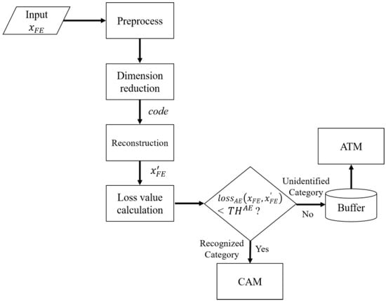
Figure 5.
Flowchart of SAM.
3.2. Classification Analysis Module (CAM)
Within the DICS framework, the SAM performs the initial classification of network packets into recognized recg and unidentified unid. unid packets are temporarily stored in a buffer, while recg packets are forwarded to the CAM for further categorization. The classification process implements both random forest and KNN algorithms, as detailed in Section 2.2 and Section 2.3, respectively, to determine the specific categories of recognized packets. Details of the CAM are shown in Figure 6.
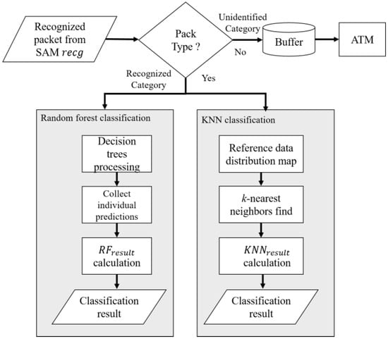
Figure 6.
Flowchart of CAM.
- Classification process using random forest.
- Step 1. Upon receiving a recg packet, each trained decision tree within the random forest ensemble processes the packet independently and generates its classification output.
- Step 2. Following the collection of individual tree predictions, the algorithm applies Equation (4) to compute the frequency distribution of predicted classes, where the most frequently occurring class is designated as the final random forest classification result.
- Classification process using KNN.
- Step 1. The behavioral features xFE of the recg packet are input into the KNN algorithm, which references these features against the trained data distribution map to identify k nearest neighboring packets.
- Step 2. After identifying the k nearest packets, the algorithm performs statistical analysis on their respective classes as formulated in Equation (5), which implements majority voting to determine the most frequent class occurrence as the final classification prediction.
Similar to the SAM described in Section 3.1, the CAM implements the agile training approach detailed in Section 3.3. The methodology leverages behavioral features from genuine unidentified packets stored in the buffer. Through this process, the CAM progressively expands its classification capabilities to encompass a broader range of packet categories.
3.3. Agile Training Module (ATM)
The primary objective of agile training is to enhance the detection capabilities of both the SAM and CAM within the DICS framework. This process utilizes unidentified packets stored in the buffer for improvement and retraining purposes. The details of agile training follow sequential steps. Details of the ATM are displayed in Figure 7.
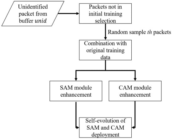
Figure 7.
Flowchart of ATM.
- Step 1. When the number of unid packets in the buffer reaches a th threshold, the ATM is activated. These packets are carefully selected, specifically targeting packets not included in the initial training of the SAM and CAM. From this filtered collection, th packets are randomly sampled to constitute the agile training dataset.
- Step 2. The Autoencoder within the SAM undergoes self-evolution learning using these th genuine unidentified packets. Upon completion of the self-evolution learning phase, the enhanced SAM model is deployed into the current system architecture.
- Step 3. For CAM enhancement, both random forest and KNN models are retrained using an augmented dataset. This dataset combines the original training data with the newly selected th unidentified packets. Following the self-evolution process, the updated random forest and KNN models are integrated into the system architecture.
Through the above comprehensive approach, DICS significantly expands its packet classification capabilities. Moreover, the training set presented in Table 1 is used to develop the fundamental model capabilities of both the SAM and CAM, as detailed in Section 3.1 and Section 3.2. The testing set from Table 1 serves to validate the recognition capabilities of the SAM and CAM under both scenarios: DICS with ATM and without ATM implementation.

Table 1.
Dataset distribution across traffic categories.
4. Experimental Results
This section presents the experimental validation of DICS. The experiments were conducted on a Windows 10 64-bit system equipped with an Intel i7-7700HQ 2.8 GHz processor (Intel Corporation, Santa Clara, CA, USA), NVIDIA GTX 1060 graphics card, and 16 GB RAM (Nvidia Corporation, Santa Clara, CA, USA). The implementation utilizes the Python 3.10.5 programming language with four essential libraries: Pandas [], NumPy [], Scikit-learn [], and TensorFlow []. In Section 4.1, the authors present information on the experimental environment. Subsequently, the DICS’s performance without the ATM is analyzed in Section 4.2. Section 4.3 then provides an in-depth analysis of the superior performance achieved after implementing the ATM.
4.1. Environment Information
To simulate real-world scenarios with maximum fidelity, this section emphasizes the rationale behind the environmental configuration. The experimental setup encompasses three aspects: dataset description and preprocessing, model architectures, and objective evaluation metrics.
4.1.1. Dataset Description and Preprocessing
DICS employs the Edge-IIoTset dataset [], which is generated from an industrial IoT testbed equipped with comprehensive sensor arrays and actuators. The testbed integrates various sensors, such as sound, temperature–humidity, ultrasonic, water level, pH, humidity, heartbeat, and flame sensors. Also, the testbed incorporates multiple actuators, such as servo motors, stepper motors, and DC motors, along with infrared receivers. The setup enables realistic industrial control system traffic simulation. The Edge-IIoTset has 15 distinct attack types commonly observed in industrial control systems, which are categorized into five attack classes plus benign traffic. The categories include man in the middle (MITM), injection attack, malware, distributed denial of service (DDoS), and information gathering, alongside benign traffic. Table 1 shows the dataset distribution of packets per category. The specific characteristics of each attack type are defined as follows.
Each packet in the dataset contains 63 initial features. The preprocessing phase involved removing 15 rule-based features, such as “ip.src”, “ip.dst”, “arp.src.proto_ipv4”, and “arp.dst.proto_ipv4”, to better reflect real-world scenarios where the identifiers vary dynamically. This elimination of environment-specific features resulted in 48 remaining features, which are more generalizable across different network contexts. Among these 48 features, seven sequential or string-based features underwent one-hot encoding transformation [], which expanded the feature set to 95 features per packet. Subsequently, packets containing null values were eliminated. To enhance model training and prediction accuracy, feature standardization [] was applied to normalize the data within the range of 0 to 1. This standardization process minimizes the impact of feature distribution variance on machine learning model performance. The dataset was partitioned into training and testing sets following the Pareto principle [], which helps prevent overfitting during the learning process.
Moreover, the authors evaluate the suitability of the selected dataset [] for industrial control system experimentation. This dataset corresponds to three fundamental requirements (FRs) specified in IEC 62443: FR 3—system integrity, FR 6—timely response to events, and FR 7—resource availability. Regarding system integrity, specifically focusing on logical asset integrity in network communications, the authors identified four relevant features from the dataset: “icmp.checksum”, “icmp.seq_le”, “tcp.checksum”, and “tcp.seq”. These protocol features are essential for verifying data integrity in industrial control systems. For FR 6, timely response to events ensures prompt detection and response to security violations without compromising system performance. Our analysis revealed seven associated elements, including features #1 (frame.time), #20 (http.tls_port), #29 (tcp.flags), #43 (dns.retransmission), #44 (dns.retransmit_request), #45 (dns.retransmit_request_in), and #53 (mqtt.msgtype). In the following, we detail the purpose and functionality of each field. The #1 field, frame.time, serves as a timestamp for recording when events occur. Field #20, http.tls_port, detects unencrypted HTTP protocol on encrypted ports, which indicates potential security vulnerabilities. Moving to #29, tcp.flags represents TCP flags that can be utilized to identify abnormal connection behaviors. Fields #43 through #45 are related to DNS operations. “dns.retransmission” flags DNS retransmissions that may indicate network issues, while “dns.retransmit_request” specifically denotes DNS query retransmissions suggesting possible network problems. Additionally, “dns.retransmit_request_in” tracks the retransmission of original requests, which is crucial for problem tracing. Field #53, mqtt.msgtype, categorizes MQTT message types for event classification. All these aforementioned fields collectively support the core functionality of FR6, which enables system monitoring, event response, and the collection and reporting of forensic evidence. As for FR 7, system resilience maintains critical safety functions during security incidents, particularly against DoS-related component unavailability. Our analysis revealed ten relevant items: #13 (http.content_length), #24 (tcp.connection.fin), #25 (tcp.connection.rst), #26 (tcp.connection.syn), #27 (tcp.connection.synack), #31 (tcp.len), #37 (udp.stream), #38 (udp.time_delta), #50 (mqtt.len), and #59 (mbtcp.len). Sequentially, we describe the functionality of each field. Field #13, http.content_length, monitors resource size through HTTP content length measurement. Regarding connection management, field #24 “tcp.connection.fin” tracks connection termination and resource release, while field #25 “tcp.connection.rst” indicates connection resets that may suggest resource issues. Furthermore, field #26 “tcp.connection.syn” monitors connection establishment requests, and field #27 “tcp.connection.synack” tracks connection establishment acknowledgments to observe connection states. Moving to data metrics, field #31 “tcp.len” represents TCP segment length for data volume monitoring. In terms of UDP communications, field #37 “udp.stream” provides UDP stream indexing for concurrent communication monitoring, and field #38 “udp.time_delta” measures the time offset from the previous frame, enabling response time analysis. For protocol-specific measurements, field #50 “mqtt.len” monitors resource utilization through message length tracking, while field #59 “mbtcp.len” oversees data volume through Modbus TCP length monitoring. These fields collectively support the critical requirements of FR7, which aims to ensure application and device availability while preventing any degradation or denial of basic services.
Conversely, the dataset encompasses identification-related information crucial for security analysis, including device communication behaviors, connection states, application layer characteristics, and industrial protocol-specific attributes. Through comprehensive integration of the above elements, the dataset provides a robust foundation for assessing security measures within an industrial control environment.
To simulate the unpredictable nature of attacks in real-world networks, the DICS framework was evaluated using four distinct experimental configurations: EG-A, EG-B, EG-C, and EG-D. Table 2 details four unique training sets. Each configuration strategically excludes one attack category during training, which reflects how different operational environments may experience varying distributions and types of attacks. Due to the sparse occurrence and unique characteristics of MITM attacks, we maintained their representation across all experimental groups. This methodology rigorously tests the capability of the system to detect previously unseen attack vectors, a critical requirement for robust intrusion detection systems. The unified test group TG comprises 381,840 network packets derived from the testing data portions, as specified in Table 1.
Table 2.
Information on testing and training sets.
4.1.2. Model Architectures
DICS incorporates two machine learning modules: SAM and CAM. Firstly, the SAM implements an Autoencoder architecture [] specifically designed for unknown traffic packet detection, as detailed in Section 3.1. The neural network configuration utilizes the sigmoid activation function across all layers, which maintains neuron values between 0 and 1 to align with the standardized feature inputs. The network architecture is structured to process 95 behavioral features, with both input and output layers containing 95 neurons to facilitate complete feature representation and reconstruction. The SAM employs a symmetric architecture with five hidden layers [], where the number of neurons in each layer is determined by progressive scaling ratios of the input dimension n: , , , , and , respectively. This progressive dimensionality reduction and expansion strategy ensures optimal feature preservation through the network layers, as detailed in Table 3. The superscript numbers indicates the layer number of the hidden layer. The number of parameters is determined according to Equation (6). Taking the value 7296 from the table as an example, 95 × 76 + 76 = 7296.
Table 3.
The configuration of SAM.
Regarding CAM, it integrates random forest and KNN algorithms to perform detailed classification of known packet clusters identified by the SAM, as described in Section 3.2. The random forest classifier is configured with 100 estimators, allowing unrestricted maximum depth and leaf nodes for full tree growth, while maintaining a minimum sample split threshold of 2. The KNN classifier employs a k-value of 5 and utilizes Euclidean distance metrics (p = 2) for proximity calculations between data points. Both classification models are implemented using the Scikit-learn framework, with all remaining parameters maintained at their default values to ensure reproducibility and standardization. As for ATM, the authors set th = 2500 based on the dataset []. In practical applications, this number of 2500 can be adjusted according to the enterprise’s packet volume capacity.
4.1.3. Objective Evaluation Metrics
The evaluation framework employs four fundamental metrics: true positive (tp), false positive (fp), true negative (tn), and false negative (fn). For comprehensive and objective assessment, these metrics form the basis for calculating Accuracy, Precision, Recall, and F-measure through Equations (7)–(10) [,]. Precision, which ranges from 0 to 1, quantifies the proportion of correct predictions among all positive predictions, while Recall measures the proportion of actual positive cases correctly identified by the model. F-measure, with β set to 1, is commonly referred to as the F1-score in classification tasks. This metric represents a harmonic mean between Precision and Recall, which indicates equal importance of both metrics in the classification performance assessment.
4.2. Performance of DICS Framework Without ATM
This section presents the experimental results of DICS without ATM. The analysis encompasses comprehensive evaluations of both SAM and CAM, which examine their performance metrics and classification effectiveness under various scenarios of unknown traffic patterns. The evaluation outcomes of the DICS classification performance are presented in Table 4a,b, which specifically focuses on the CAM architecture utilizing random forest as the traffic packet classifier.
Table 4.
Performance metrics of dual models without ATM: (a) DICS employing random forest; (b) DICS employing KNN.
Despite achieving a high accuracy of 0.99, this metric in Table 4 is misleading due to dataset imbalance. Benign traffic significantly outnumbers attack traffic in our dataset, which reflects real-world network conditions, as described in Section 4.1.3. Thus, here, Precision, Recall, and F1-score serve as more meaningful performance indicators with most values falling below 0.8, which reveals substantial limitations. These lower values demonstrate that DICS without ATM requires significant improvement in identifying critical minority classes that represent actual attack patterns. The evaluation metrics for EG-C showed superior performance, with values exceeding 0.97 across all measures. The reason is that EG-C specifically excluded malware attacks, in which malware inherently functions as a composite attack vector that integrates techniques from multiple attack categories. Such integration creates significant feature overlap with other attack types. When operating without the ATM, DICS exhibited performance limitations in EG-A, EG-B, and EG-D scenarios. In these environments, unidentified traffic packets were incorrectly classified as recognized packets, which led to subsequent categorization errors when processed by the CAM.
The authors further examine the performance of individual DICS modules functioning without the ATM component. This analysis comprises two parts: an evaluation of SAM effectiveness without ATM in Section 4.2.1, followed by an examination of CAM performance in Section 4.2.2.
4.2.1. Evaluation of SAM Without ATM
This section presents the effectiveness of the SAM without ATM conditions, which corresponds to A.a and A.b, as illustrated in Figure 4. The outcomes are summarized in Table 5a,b, with gray-highlighted categories indicating traffic patterns intentionally excluded from the initial training. These unidentified traffic types were incorporated to create realistic testing scenarios that mirror actual deployment environments, as outlined in Section 4.1.3. A closer examination of Table 5a reveals substantial quantities of gray-highlighted categories, which indicates the response of the system before ATM implementation. Without the ATM, the SAM predominantly categorizes unfamiliar packets as unidentified packet groups. Additionally, a minimal fraction of previously unlearned packets was erroneously classified as recognized packets, as demonstrated in Table 5b. Specifically, EG-A, EG-B, and EG-D exhibited misclassification counts of 3103, 22,078, and 2288 packets, respectively.
Table 5.
Packet groups identified by SAM without ATM. (a) Unidentified packet group; (b) recognized packet group.
To emphasize the binary classification capability of SAM, the authors conducted an evaluation using the area under the curve (AUC) metric through Equations (11)–(13). Although SAM exhibited minimal identification errors without the ATM, its effectiveness requires further validation. The AUC value, which ranges from 0 to 1, provides this validation by assessing the ability of the system to distinguish between “Unidentified packets” and “Recognized packets”, where a value approaching 1 indicates superior model classification performance. As shown in Table 6, EG-A through EG-D achieved impressive AUC scores of 0.977, 0.945, 1.000, and 0.971, respectively. Therefore, we can confirm the effective deployment of SAM across all test scenarios.
Table 6.
AUC values across experimental groups.
4.2.2. Evaluation of CAM Without ATM
Following the packet segregation by SAM into recognized and unidentified packet groups, CAM performs classification on each traffic packet within the recognized packet groups. This section presents CAM classification results prior to ATM mechanism implementation, which is evaluated using objective metrics from Section 4.1.3: Precision and Recall, as defined by Equations (8) and (9). The CAM employs two models: random forest and KNN, as detailed in Section 3.2. Table 7a–d present the experimental results for each group, where an NaN value indicates the absence of specific traffic packet types in the known packet groups. Notably, Accuracy was deliberately excluded as an evaluation metric due to the disproportionate representation of the benign class in the test set, which could potentially skew the analysis of classification effectiveness. Gray-highlighted categories represent genuinely unknown packet types for the respective experimental groups. The average values of Precision and Recall are derived by Equations (14) and (15), respectively.
Table 7.
Without-ATM classification metrics across experimental groups using dual models: (a) EG-A; (b) EG-B; (c) EG-C; (d) EG-D.
In Table 7a,b,d, all gray-highlighted categories show zero values. This outcome reflects the inability of CAM to identify these packet types, as they were absent during the initial training phase, and the system lacks a self-learning mechanism. Table 7c displays NaN for the gray-highlighted “Malware” category because SAM directed all such packets to the unidentified packet buffer, which prevented CAM from receiving any malware packets for classification. Similarly, the MITM category in Table 7a,b,c shows NaN values due to the SAM screening in the first-layer DICS. MITM packets were categorized into the unidentified packet group. Thus, this prevented any MITM traffic from reaching the CAM component. For the Average calculation, we computed the mean of non-NaN values within each row. For example, in Table 7a, the average Precision for random forest is calculated as (0.9507 + 1.0000 + 0.9572 + 0 + 1.0000)/5 = 0.7816, which excludes NaN entries from the calculation. Significantly, EG-C maintained a high average value of 0.9841. This is because this experimental group was designed to minimize malware influence, which typically exhibits overlapping packet characteristics with other attack types. In this scenario, SAM successfully fulfilled its objective by filtering these attack types into the unidentified packet group. While EG-C demonstrated promising results, the other three experimental groups achieved average values below 0.8, which indicates a clear need for enhanced attack classification capabilities. Regardless of which model was implemented in CAM, all classification results require substantial improvement. This limitation necessitates further optimization of the underlying algorithms for effective threat detection.
4.3. Performance DICS Framework After Implementing ATM
This section validates the effectiveness of integrating the ATM into the DICS framework. The buffer illustrated in Figure 4 enables the system to collect and perform agile training on genuinely unidentified packet categories. This training process enhances the recognition capabilities of SAM while reducing the misclassification rates in the CAM. The experimental outcomes are evaluated using the same metrics as Section 4.1.3: Accuracy, Precision, Recall, and F1-score. Table 8 presents the performance metrics of ATM implementation under dual models across EG-A through EG-D.
Table 8.
Performance metrics of ATM under dual models across EG-A~D: (a) DICS employing random forest; (b) DICS employing KNN.
Table 8 exhibits substantial improvements compared to Table 4. The CAM maintained high accuracy values exceeding 0.98 across both random forest and KNN implementations. In the EG-B scenario, accuracy increased to over 0.94. This enhancement stems from the agile training module that stores unrecognized packets in a buffer for periodic analysis and identification. Under imbalanced dataset conditions, metrics such as Precision, Recall, and F1-score provide more reliable performance indicators. The examination of Precision, Recall, and F1-score metrics shows considerable performance gains across most experimental groups. The EG-C scenario, however, exhibited slight performance decreases rather than enhancement. This decline occurred primarily because the capability of DICS to identify malware based on packet characteristics affected overall effectiveness. Nevertheless, all results still remained above 0.95. After all, the random forest implementation in the CAM consistently outperformed KNN across all scenarios. While KNN performance was comparatively lower, it still maintained metrics above 0.85 across all scenarios. As for random forest, all evaluation metrics exceeded 0.97 in all experimental groups except EG-B.
For a comprehensive evaluation, the following sections present detailed analyses of SAM performance under ATM scenarios in Section 4.3.1 and CAM classification capabilities after ATM implementation in Section 4.3.2.
4.3.1. Evaluation of SAM Under ATM Scenario
This section employs identical training datasets for SAM and CAM initialization as those used in Section 4.2.1, along with the same test datasets for validation purposes. The key distinction lies in the implementation of the agile training module, as described in Section 3.3, which utilizes buffered traffic packets to continuously evolve and enhance the learning capability of the SAM. This capability expands the range of identifiable traffic patterns beyond the initial training scope, which allows the system to adapt to emerging threats. To thoroughly analyze the benefits of the ATM, we conducted an ablation study comparing the performance of the SAM both with and without ATM functionality. The detection results for various attack types using the SAM without the ATM are documented in Table 5, while the experimental results after implementing the ATM are presented in Table 9. The gray-highlighted categories indicate the original unidentified traffic packets for each experimental group. These gray sections correspond to the simulated real-world environment scenarios, as described in Table 3.
Table 9.
Packet groups identified by SAM with ATM: (a) unidentified packet group; (b) recognized packet group.
Table 9a displays the unidentified packet clusters detected by the SAM, while Table 9b shows the recognized packet groups. After that, we can observe that packets initially classified as unidentified packet groups are shown in Table 5a. Through the agile training process, the majority of previously unidentified traffic categories are successfully reclassified into recognized packet groups. This transformation is evidenced by the increased number of identifiable packets in the gray-highlighted sections of Table 9b. This marked improvement can be attributed to the ATM’s capability to redirect genuine unknown traffic patterns back to the SAM model for self-learning and continuous adaptation. This can enhance its classification capability for recognized packet categories.
4.3.2. Evaluation of CAM Under ATM Scenario
This section presents a comparative analysis of CAM performance in DICS with agile training module integration. The SAM in DICS initially segregates incoming traffic packets into recognized and unidentified packet groups, with recognized packets being subsequently processed by the CAM for classification. The analysis methodology differs from Section 4.2.2 in two aspects: recognized packet groups are processed through an enhanced learning SAM as outlined in Section 4.3.1. Additionally, the CAM incorporates retraining to accommodate a broader spectrum of traffic packet classifications. The performance evaluation metrics maintain consistency with Section 4.2.2, which utilizes Precision and Recall as primary indicators, as illustrated in Table 10. The average values of Precision and Recall in Table 10 are derived by Equations (14) and (15), respectively.
Table 10.
ATM classification metrics across experimental groups by CAM using different models (a) EG-A; (b) EG-B; (c) EG-C; (d) EG-D.
A key distinction from Section 4.3.2 lies in the exclusive use of traffic packets processed by the agile training-enhanced SAM, with all classified packet types aligning to the retrained CAM classification framework. The experiments encompass comparative analyses between random forest and KNN classifiers, which simulate their respective classification effectiveness. The integration of ATM functionality significantly improved the overall recognition performance across all experimental groups. Attack categories highlighted in gray that remained unidentifiable in Table 7 demonstrate Precision and Recall values above 0.96 in dual models when implementing the ATM mechanism, as shown in Table 10. Regarding the EG-B configuration, the outcomes show comparatively lower performance metrics among the experimental groups. The reason for the limitation originates from its initial exclusion of DDoS attacks, which created specific challenges in attack classification. Although the ATM mechanism successfully enabled high recognition rates for previously unlearned DDoS attacks, misclassifications occurred between injection and information-gathering attacks. The Precision rates for these attack types reached only 0.682 and 0.580, respectively. This confusion results from their sequential relationship in attack chains, where information gathering typically serves as the initial reconnaissance phase before injection attacks are executed. From a model perspective, the random forest algorithm in CAM demonstrated superior performance compared to KNN, which achieved average precision and recall values of 0.9592 and 0.9808. We can learn from the experiments’ outcomes that the ATM approach expands the variety of categories that the CAM can classify.
In the last part, the integration of the ATM mechanism significantly enhanced classification capabilities by expanding the range of recognizable attack categories. As shown in Table 11, while performance improvements varied between experimental groups, the most substantial gains were observed in previously unidentifiable attack types. DICS successfully increases the number of categories within recognized packet groups output by the SAM and strengthens the classification capability of the CAM for various attack types. Consequently, the authors firmly validate the practical feasibility of the DICS in handling diverse network traffic patterns.
Table 11.
ATM classification metrics across experimental groups using different models: (a) EG-A; (b) EG-B; (c) EG-C; (d) EG-D.
5. Conclusions and Future Works
The authors have designed a diverse machine learning-based malicious attack detection system for industrial control environments. DICS employs a two-module approach where the first detection module, SAM, preliminarily identifies unknown traffic at the IT-OT boundary. The second module, CAM, then classifies this traffic into specific types. Benign packets are allowed to proceed to the internal industrial control domain, while the system is immediately alerted upon detection of malicious flows. Also, the proposed scheme incorporates agile training capabilities through periodic aggregation of unidentifiable traffic packets from the SAM. These collected packets update both detection modules with new data, which enables continuous system self-improvement. The experimental outcomes using datasets encompassing information from various industrial control sensors demonstrate excellent performance in both SAM and CAM components. Significant numerical improvements have been observed when comparing pre- and post-agile training implementation, which confirms the effectiveness of DICS for traffic boundary protection in the industrial control environment. In future works, the authors will explore industrial cybersecurity standards, with a specific focus on IEC 62443 security requirements. The authors also plan to extend experimental validation by testing the framework across multiple models. Future work will advance to the next phase of the AI lifecycle, which emphasizes operational deployment considerations. This includes evaluating system integration, establishing monitoring metrics, and developing long-term maintenance strategies.
Author Contributions
Conceptualization, C.-H.C.; Methodology, Y.-C.C.; Validation, J.-S.L.; Investigation, C.-H.C.; Data curation, T.-W.L.; Writing—original draft, Y.-C.C. All authors have read and agreed to the published version of the manuscript.
Funding
This research received no external funding.
Data Availability Statement
Data are contained within the article.
Conflicts of Interest
The authors declare no conflict of interest.
References
- Mourtzis, D. 2-Industry 4.0 and Smart Manufacturing. In Manufacturing from Industry 4.0 to Industry 5.0, Advances and Applications; Elsevier: Amsterdam, The Netherlands, 2024; pp. 13–61. [Google Scholar]
- A Comprehensive Guide to Digital Transformation in Manufacturing. Available online: https://www.themanufacturer.com/articles/a-comprehensive-guide-to-digital-transformation-in-manufacturing/ (accessed on 10 March 2025).
- The 7 Top Smart Manufacturing Trends to Watch in 2025. Available online: https://archerpoint.com/smart-manufacturing-trends-for-2025/ (accessed on 10 March 2025).
- Lee, J.S.; Chen, Y.C.; Chew, C.J.; Hong, W.Z.; Fan, Y.Y.; Li, B. Constructing Gene Features for Robust 3D Mesh Zero-watermarking. JISA 2023, 73, 103414. [Google Scholar] [CrossRef]
- Chew, C.J.; Lee, W.B.; Sung, L.Z.; Chen, Y.C.; Wang, S.J.; Lee, J.S. Lawful Remote Forensics Mechanism with Admissibility of Evidence in Stochastic and Unpredictable Transnational Crime. IEEE TIFS 2024, 19, 5956–5970. [Google Scholar] [CrossRef]
- Chin, Y.C.; Hsu, C.L.; Lin, T.W.; Tsai, K.Y. Dynamic Trust Management Framework using Blockchain for Zero-Trust-based Authentication in BYOD Environments. Enterp. Inf. Syst. 2025, 19. Available online: https://www.tandfonline.com/doi/full/10.1080/17517575.2025.2457952 (accessed on 10 March 2025).
- Lee, J.S.; Chen, Y.C.; Chew, C.J.; Chen, C.L.; Huynh, T.N.; Kuo, C.W. CoNN-IDS: Intrusion Detection System based on Collaborative Neural Networks and Agile Training. Comput. Secur. 2022, 122, 102908. [Google Scholar] [CrossRef]
- ISA/IEC 62443 Series of Standards. Available online: https://www.isa.org/standards-and-publications/isa-standards/isa-iec-62443-series-of-standards (accessed on 10 March 2025).
- Dolezilek, D.; Gammel, D.; Fernandes, W. Cybersecurity based on IEC 62351 and IEC 62443 for IEC 61850 systems. In Proceedings of the 15th International Conference on Developments in Power System Protection (DPSP 2020), Liverpool, UK, 9–12 March 2020. [Google Scholar]
- Franceschett, A.L.; de Souza, P.R.A.; de Barros, F.L.P.; de Carvalho, V.R. A Holistic Approach—How to Achieve the State-of-art in Cybersecurity for a Secondary Distribution Automation Energy System Applying the IEC 62443 Standard. In Proceedings of the 2019 IEEE PES Innovative Smart Grid Technologies Conference—Latin America (ISGT Latin America), Gramado, Brazil, 15–18 September 2019. [Google Scholar]
- Siemens Gains IEC 62443 Certification for Secure System Integration Services. Available online: https://press.siemens.com/global/en/pressrelease/siemens-gains-iec-62443-certification-secure-system-integration-services (accessed on 10 March 2025).
- The NIST Cybersecurity Framework (CSF) 2.0. Available online: https://nvlpubs.nist.gov/nistpubs/CSWP/NIST.CSWP.29.pdf (accessed on 10 March 2025).
- OneHotEncoder. Available online: https://scikit-learn.org/stable/modules/generated/sklearn.preprocessing.OneHotEncoder.html (accessed on 10 March 2025).
- Ho, T.K. Random Decision Forests. In Proceedings of the 3rd International Conference on Document Analysis and Recognition, Montreal, QC, Canada, 14–16 August 1995; Volume 2, pp. 278–282. [Google Scholar]
- Altman, N. An Introduction to Kernel and Nearest-neighbor Nonparametric Regression. Am. Stat. 1990, 46, 175–185. [Google Scholar] [CrossRef]
- Kramer, O. Scikit-learn. In Machine Learning for Evolution Strategies; Springer: Cham, Switzerland, 2016; Volume 20, pp. 45–53. [Google Scholar]
- Mckinney, W. Data Structures for Statistical Computing in Python. In Proceedings of the 9th Python in Science Conference, Austin, TX, USA, 28 June–3 July 2010; Volume 445, pp. 51–56. [Google Scholar]
- Harris, C.R.; Millman, K.J.; van der Walt, S.J.; Gommers, R.; Virtanen, P.; Cournapeau, D.; Wieser, E.; Taylor, J.; Berg, S.; Smith, N.J.; et al. Array Programming with NumPy. Nature 2020, 585, 357–362. [Google Scholar] [CrossRef] [PubMed]
- TensorFlow Distributions. Available online: https://arxiv.org/abs/1711.10604 (accessed on 10 March 2025).
- Ferrag, M.A.; Friha, O.; Hamouda, D.; Maglaras, L.; Janicke, H. Edge-IIoTset: A New Comprehensive Realistic Cyber Security Dataset of IoT and IIoT Applications for Centralized and Federated Learning. IEEE Access 2022, 10, 40281–40306. [Google Scholar] [CrossRef]
- Alqahtani, A.; Whyte, A. Estimation of Life-cycle Costs of Buildings: Regression vs Artificial Neural Network. Built Environ. Proj. Asset Manag. 2016, 6, 30–43. [Google Scholar] [CrossRef]
- Salahuddin, M.; Pourahmadi, V.; Alameddine, H.; Bari, M.; Boutaba, R. Chronos: DDoS Attack Detection using Time-based Autoencoder. IEEE TNSM 2022, 19, 627–641. [Google Scholar] [CrossRef]
- Stiawan, D.; Susanto; Bimantara, A.; Idris, M.Y.; Budiarto, R. IoT Botnet Attack Detection using Deep Autoencoder and Artificial Neural Networks. KSII Trans. Internet Inf. Syst. 2023, 17, 1310–1338. [Google Scholar]
- Cui, J.; Sun, H.; Zhong, H.; Zhang, J.; Wei, L.; Bolodurina, I.; He, D. Collaborative Intrusion Detection System for SDVN: A Fairness Federated Deep Learning Approach. IEEE Trans. Parallel Distrib. Syst. 2023, 34, 2512–2528. [Google Scholar] [CrossRef]
- Mehedi, S.T.; Anwar, A.; Rahman, Z.; Ahmed, K.; Islam, R. Dependable Intrusion Detection System for IoT: A Deep Transfer Learning based Approach. IEEE Trans. Ind. Inform. 2023, 19, 1006–1017. [Google Scholar] [CrossRef]
Disclaimer/Publisher’s Note: The statements, opinions and data contained in all publications are solely those of the individual author(s) and contributor(s) and not of MDPI and/or the editor(s). MDPI and/or the editor(s) disclaim responsibility for any injury to people or property resulting from any ideas, methods, instructions or products referred to in the content. |
© 2025 by the authors. Licensee MDPI, Basel, Switzerland. This article is an open access article distributed under the terms and conditions of the Creative Commons Attribution (CC BY) license (https://creativecommons.org/licenses/by/4.0/).