An Extended Method for Reversible Color Tone Control Using Data Hiding

Abstract

This paper proposes an extended method for reversible color tone control for blue and red tones. Our previous method has an issue in that there are cases where the intensity of enhancement cannot be flexibly controlled. In contrast, the proposed method can gradually improve the intensity by increasing the correction coefficients, regardless of the image features. This is because the method defines one reference area where the correction coefficients are determined, one each for blue and red tones, while the previous method defines a common reference area for both tones. Owing to this, the method also provides independent control for blue and red tones. In our experiments, we clarify the above advantages of the method. Additionally, we also discuss the influence of the data-embedding process, which is necessary to store recovery information, on the output image quality.

1. Introduction

Image-processing applications have been more commonly used with the development of smartphones and social networking services (SNSs). With common image-processing methods, it is difficult to simply restore an original image from a processed image. If the original image is also required, the processing history or the original image itself needs to be stored separately from the processed image. Although many image-restoration methods have been proposed [1,2], it is difficult to restore an image without tolerating even a single bit error. Recently, image restoration using deep learning was also proposed [3,4], but most of these methods allow for some errors compared with the original image. In addition, the operations are complex, and the processing cost increases significantly. To address this issue, contrast-enhancement methods that guarantee reversibility by using data hiding were proposed [5,6,7,8,9,10,11,12,13,14]. Wu et al. proposed a method for grayscale images that uses histogram shifting [5]. In this method, we embed information that is necessary for restoration (hereafter called recovery information) into an image histogram, and the original image can be reconstructed by using the recovery information. However, this method may cause a significant difference in the average luminance of the entire image between before and after processing. To tackle this issue, reversible contrast-enhancement methods without differences in the average luminance were studied [12,13,14]. For instance, Wu et al. introduced a two-dimensional histogram-to-histogram shifting so that the average luminance can be controlled while enhancing the contrast [14]. However, these methods focus on grayscale images. If these methods are directly applied to color images, visible hue distortion may appear.

Recently, several image-processing methods were proposed for color images [15,16,17]. They can preserve the hue component by referencing the HSV color space. Wu et al. first proposed a method that enhances the contrast without hue degradation [15]. However, in the restoration process, the original image cannot be perfectly retrieved, and thus, an image analogous to the original is reconstructed. Sugimoto et al. then proposed another method that guarantees perfect reversibility by embedding recovery information [17]. Additionally, this method can perform not only contrast enhancement but also multiple types of processing, such as sharpening/smoothing and saturation improvement, without causing hue distortion. However, with this method, hue control is not taken into account.

Thus, we focused on the hue component as a control object. We previously proposed a reversible method that can control the blue or red tones of an image [18]. The method targets blue and red tones to control the coldness or warmth of an image. In our previous method, we adopted the YDbDr color space [19] used in JPEG 2000 [20] instead of the HSV color space. A reference area is first defined in the $D_b$–$D_r$ plane. Correction coefficients are then calculated within the reference area. Finally, the RGB components are multiplied by these coefficients so that a tone-enhanced image is derived. However, in some cases, the intensity of the enhancement could not be controlled due to severe variations in the pixel values or the distribution of pixels being inconvenient within the reference area.

In this paper, we propose an effective extension of the reversible tone-enhancement method [18]. This method is strongly expected to be a new breakthrough in terms of storage saving in image processing with limited storage environments, including devices such as smartphones and tablets. The proposed tone-enhancement method offers two main contributions. One of them is that the method is effective for every image, regardless of the image features. In the previous method, tone enhancement is not effective for some images. The other contribution is that the method allows for the gradual control of the intensity of enhancement, regardless of the image features. The previous method does not gradually control the intensity of the enhancement, and thus, the intensity changes abruptly. In addition, the intensity of the enhancement limit is reached in the early stage of the enhancement control for some images. The proposed method solves both of the above issues. It can calculate correction coefficients without being affected by variations in pixel values within the reference areas. Each of the correction coefficients can be separately obtained in each of the reference areas. This allows for independent control of both tones, and thus, the intensity of the enhancement limit can be expanded. Recovery information is embedded into an image using the reversible data-hiding method. In our experiments, the correction coefficients were compared with those of the previous method in order to clarify that the intensity of enhancement can be flexibly controlled. Additionally, we evaluated the influence of the data-embedding process on the output image quality.

2. Reversible Color Tone Control Method

We previously proposed a unique method that allows us to reversibly enhance blue or red tones of color images [18]. In this method, we calculate a correction coefficient for each color component and then enhance the color tone by multiplying the coefficients by each pixel value. In the following, we describe the procedure in detail and challenges of this method.

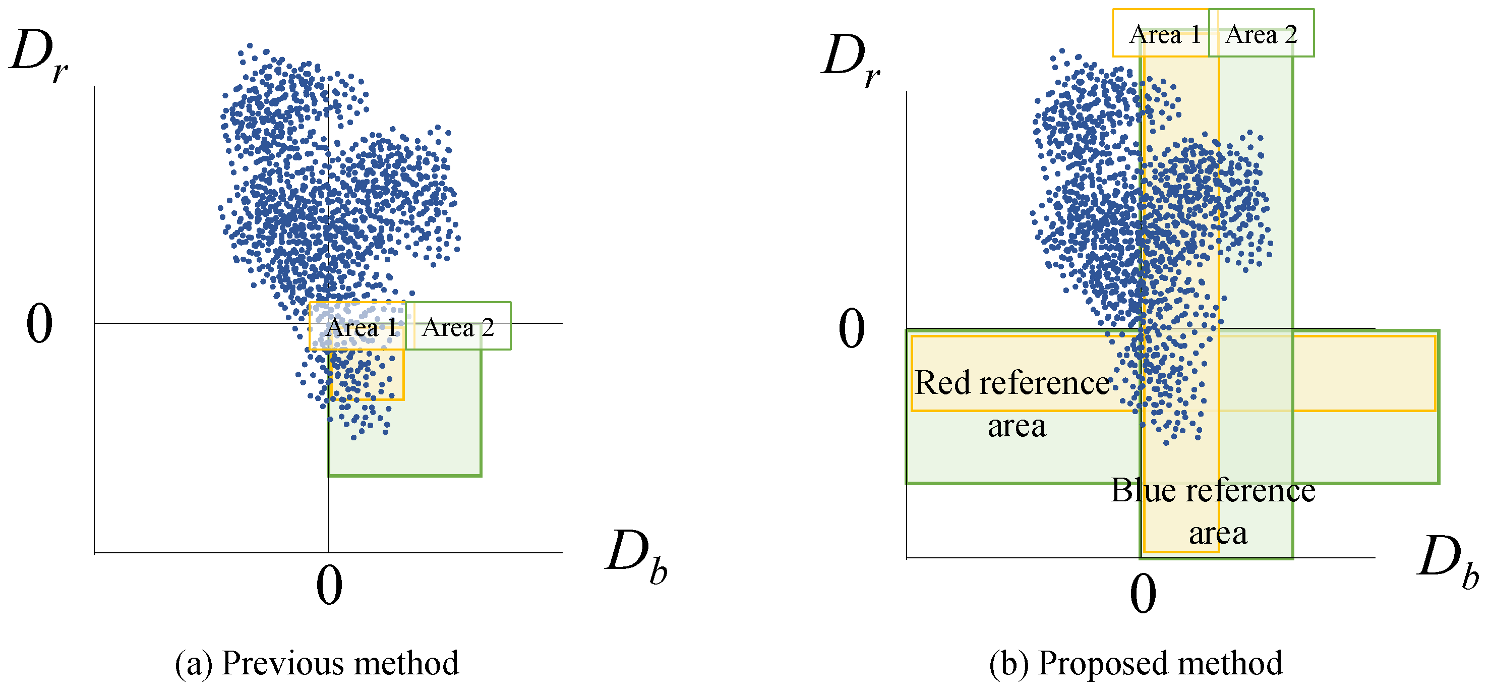
2.1. Procedure of Previous Method

In this method, we refer to the ${\mathrm{YD}}_{\mathrm{b}}{\mathrm{D}}_{\mathrm{r}}$ color space in order to control blue or red tones. The ${\mathrm{YD}}_{\mathrm{b}}{\mathrm{D}}_{\mathrm{r}}$ color space is a color transform that is reversible from the RGB color space and used in JPEG 2000 [20], which is an international standard for image compression. This ${\mathrm{YD}}_{\mathrm{b}}{\mathrm{D}}_{\mathrm{r}}$ color space is different from the common ${\mathrm{YD}}_{\mathrm{b}}{\mathrm{D}}_{\mathrm{r}}$ color space. Specifically, it is converted from the RGB color space, with integer values for the reversibility. The color space consists of the luminance Y, blue tone component $D_b$, and red tone component $D_r$. The RGB-to-${\mathrm{YD}}_{\mathrm{b}}{\mathrm{D}}_{\mathrm{r}}$ and ${\mathrm{YD}}_{\mathrm{b}}{\mathrm{D}}_{\mathrm{r}}$-to-RGB transforms are given by

$$\left[\begin{array}{c}Y\\ D_b\\ D_r\end{array}\right]=\left[\begin{array}{ccc}1/4& 1/2& 1/4\\ 1& -1& 0\\ 0& -1& 1\end{array}\right]\left[\begin{array}{c}R\\ G\\ B\end{array}\right],$$

(1)

$$\left[\begin{array}{c}R\\ G\\ B\end{array}\right]=\left[\begin{array}{ccc}1& 3/4& -1/4\\ 1& -1/4& -1/4\\ 1& -1/4& 3/4\end{array}\right]\left[\begin{array}{c}Y\\ D_b\\ D_r\end{array}\right].$$

(2)

The previous method attains reversible tone control by multiplying the correction coefficients by each pixel value. Before calculating the correction coefficients, we first define a reference area in the $D_b$–$D_r$ plane. In this method, the average color within the reference area should be achromatic after the tone control. Here, the reference area means the area in which the average color will be achromatic after processing. Figure 1 shows a scatter plot of pixels in the $D_b$–$D_r$ plane and examples of the reference area. In the case of blue enhancement, the reference area should be defined in the second quadrant. In the case of red enhancement, the reference area should be defined in the fourth quadrant.

Figure 1. Scatter plot of pixels in $D_b$–$D_r$ plane and examples of reference areas.

Next, we derive the mean values of R, G, B, and Y to obtain the $R_{ave}$, $G_{ave}$, $B_{ave}$, and $Y_{ave}$ of the pixels belonging to the reference area, respectively. $R_{ave}$, $G_{ave}$, and $B_{ave}$ are rounded to integers. The correction coefficients $K_r$, $K_g$, and $K_b$ for each R, G, and B component are obtained by

$$\left\{\begin{array}{c}\begin{array}{c}\hfill K_r=\frac{Y_{ave}}{R_{ave}}\\ \hfill K_g=\frac{Y_{ave}}{G_{ave}}\\ \hfill K_b=\frac{Y_{ave}}{B_{ave}}\end{array}\hfill \end{array}\right..$$

(3)

$K_r$, $K_g$, and $K_b$ are multiplied by every pixel value, resulting in color tone enhancement. Throughout our experiments, we found that $K_g$ consistently takes a value close to 1.0, regardless of the reference area taken. In other words, $K_g$ has little influence on the tone control. Therefore, the previous method regards $K_g$ as a constant of 1.0 to reduce the recovery information.

In this method, recovery information is required to completely reconstruct the original image. For example, $R_{ave}$, $G_{ave}$, and $B_{ave}$ should be stored to reclaim $K_r$, $K_g$, and $K_b$ on the restoration side. Therefore, $R_{ave}$, $G_{ave}$, and $B_{ave}$ used in the calculation of correction coefficients need to be stored as recovery information. Such recovery information is embedded into the image itself using the reversible data-hiding method.

2.2. Challenge with Previous Method

In the previous method, the intensity of the enhancement can be controlled by adjusting the size and position of the reference area. However, in some cases, control of the intensity of enhancement is not possible. Figure 2 shows an example of this issue.

Figure 2. Ineffective control with previous method [18].

There are two factors for this.

The first factor is the variation in the R, G, and B values of each pixel belonging to the reference area. As can be seen from Equation (1), even if certain pixels in the reference area have the same value for $D_b$ and/or $D_r$, their R, G, and B values are not necessarily the same. In fact, their R, G, and B values might be completely different. Nevertheless, according to Equation (3), each correction coefficient is obtained as the ratio of $Y_{ave}$ to $R_{ave}$, $G_{ave}$, or $B_{ave}$. Therefore, even among reference areas with the same mean value for $D_b$ and $D_r$, the correction coefficients will be different, and the enhancement effect will be also different. However, the previous method cannot control the variations in R, G, and B values because the reference area is defined in the $\mathrm{Y}{\mathrm{D}}_{\mathrm{b}}{\mathrm{D}}_{\mathrm{r}}$ color space. This prevents us from flexibly enhancing the color tone to the desired intensity.

Another factor is that every correction coefficient is derived from a single reference area. In the previous method, the intensity of the enhancement is generally improved by enlarging the reference area. To improve the intensity of the enhancement, $K_r$ should become larger, while $K_b$ should become smaller. In contrast, Figure 3 shows an example of red enhancement with less effective control. In this figure, two reference areas with different sizes are defined. Comparing the two areas, Area 2 contains more pixels with a small value of $D_r$. Thus, $K_r$ should increase more effectively in Area 2. However, Area 2 does not contain pixels with a larger value of $D_b$ compared with Area 1. Therefore, the mean value of $D_b$ in Area 2 is not larger than that in Area 1, and thus, $K_b$ never decreases. Consequently, the red tone is adequately enhanced by enlarging the reference area, while the blue tone is not suitably suppressed. This interferes with the uniform control of the intensity of the enhancement.

Figure 3. Options for reference area in case of red enhancement with previous method [18].

In this paper, we tackle the issue with the previous method in consideration of these factors and attain more uniform and gradual control of the intensity of enhancement regardless of the image features.

3. Proposed Method

In this section, we propose an extension method that enables the uniform and gradual control of the intensity of the enhancement and independent control of each color tone, regardless of the image features. In the proposed method, the correction coefficients for blue and red tones are calculated separately. In addition, the correction coefficients can be obtained without being affected by variations in the pixel values belonging to the reference area. The following sections describe each procedure for the tone control and restoration processes of the proposed method, and we finally summarize the advantages of our method.

3.1. Tone Control Process

We first explain the procedure of our new tone control method in detail. As shown in Figure 4, the process consists of three steps: derivation of the correction coefficients, update pixel values, and data embedding. Each step is described below.

Figure 4. Block diagram of tone control process.

3.1.1. Derivation of Correction Coefficients

First, the RGB color space is converted to the ${\mathrm{YD}}_{\mathrm{b}}{\mathrm{D}}_{\mathrm{r}}$ color space by using Equation (1). We then define the reference areas in the $D_b$–$D_r$ plane to derive blue and red correction coefficients $K_b$ and $K_r$, which are represented as the blue reference area and the red reference area. Figure 5 shows an example of each reference area in the $D_b$–$D_r$ plane. As shown in this figure, each reference area is defined as a rectangle, and the intensity of the enhancement can be controlled by changing the position and size of these rectangles. In the proposed method, the blue reference area is controlled by the parameters $x_1$ and $x_2$, while the red reference area is controlled by the parameters $y_1$ and $y_2$. In the case of blue enhancement, the blue reference area is defined in the negative value area of $D_b$, and the red reference area is defined in the positive value area of $D_r$. In contrast, in the case of red enhancement, each area is defined opposite to the blue enhancement case. The intensity for the blue tone can be improved by changing the blue reference area to include pixels located further away from the y-axis; the intensity for the red tone can be improved by changing the red reference area to include pixels located further away from the x-axis.

Figure 5. Definition of blue and red reference areas in the case of red enhancement.

Next, the correction coefficients are calculated by using the mean value of the pixels belonging to each reference area. We derive the mean values of $D_b$ and $D_r$, called $D_{b_{areaB}}$ and $D_{r_{areaR}}$, from the blue and red reference areas, respectively. We also obtain the mean value of G, called $G_{img}$, from the image. $G_{img}$ is rounded to an integer value, and $D_{b_{areaB}}$, $D_{r_{areaR}}$, and the rounded value of $G_{img}$ are stored as recovery information.

Finally, the correction coefficients $K_b$ and $K_r$ for the B and R components are given by

$$\left\{\begin{array}{c}\begin{array}{c}\hfill K_b=\frac{G_{img}}{D_{b_{areaB}}+G_{img}}\\ \hfill K_r=\frac{G_{img}}{D_{r_{areaR}}+G_{img}}.\end{array}\hfill \end{array}\right.$$

(4)

On the basis of Equation (1), $D_b$/$D_r$ is obtained as the difference between the G component and the B/R component. Therefore, as shown in Equation (4), the correction coefficients for reducing the blue or red tones from the reference areas can be derived by using the G component. However, in the case where the number of pixels in each reference area is small, the mean value of the G component in the area may be extremely large or small. If we use such a mean value for the G component, the wrong correction coefficients are obtained. The proposed method thus calculates the correction coefficients using the mean value of the G component calculated from the entire image.

3.1.2. Update Pixel Values

In the proposed method, overflows may be caused by multiplying pixel values by the correction coefficients $K_r$ and $K_b$. We need to carry out preprocessing to prevent such overflows. First, we obtain the maximum pixel value Pmax that never causes overflows, even when multiplied by $K_r$ and $K_b$. For example, in the case of red enhancement, $P_{max}$ is given by

$$P_{max}=\lfloor \frac{255}{K_r}\rfloor .$$

(5)

Pixels with values exceeding $P_{max}$ should cause overflows. Thus, we replace such pixels with $P_{max}$. The locations of the replaced pixels and their differences from $P_{max}$ are stored as recovery information. After the preprocessing, the R and B components are multiplied by $K_r$ and $K_b$. The multiplied R and B are rounded to integers, and an intermediate image with an enhanced tone is derived. We should note that pixel locations with errors caused by rounding are stored in a location map. The maximum error value is 1. In the case that a pixel has an error, 1 is recorded in the location map. Contrarily, in the case that the pixel does not have an error, 0 is recorded. The location map is a binary image with the same size as the original image itself. The location map is thus compressed using JBIG2 [21], which is an international standard for binary image coding.

3.1.3. Data Embedding

For perfect reversibility, we need to embed all recovery information into the intermediate image. The G component provides a large contribution to the luminance, that is, it has a large visual impact; therefore, we should avoid embedding the recovery information into the G component. In the case of blue enhancement, we embed recovery information into the R component using the reversible data-hiding method; conversely, we embed it into the B component in the case of red enhancement. For our method, we use the prediction error expansion with histogram shifting (PEE-HS) method [22], but arbitrary methods can also be adopted. One-bit data for identifying the component containing the recovery information is embedded into the least significant bit (LSB) of the top-left pixel in the G component. The LSB is replaced with 1 in the case of red enhancement and 0 in the case of blue enhancement. Finally, we obtain an output image through this data-embedding process. Note that the original LSB should also be stored as recovery information. In the restoration process, this bit is first referenced to identify the marked component, i.e., the component that contains the recovery information. The recovery information consists of the following: $D_{b_{areaB}}$; $D_{r_{areaR}}$; the rounded value of $G_{img}$; the information for the preprocessing, e.g., the compressed location map described in Section 3.1.2; the original LSB in the G component; and the information on rounding errors. This information enables the original image to be perfectly restored.

3.2. Restoration Process

We can perfectly restore the original image from the output image with this method. As shown in Figure 6, the restoration process consists of three steps: data extraction, re-derivation of the correction coefficients, and recovery of the original pixel values.

Figure 6. Block diagram of restoration process.

3.2.1. Data Extraction

We first identify the marked component by referring to the LSB of the top-left pixel in the G component. We then extract the recovery information including the original bit of the LSB. An intermediate image is reconstructed by replacing the LSB with the original. The recovery information extracted here is necessary for the processes described in Section 3.2.2 and Section 3.2.3. We should note that in the proposed method including other related work, the recovery information cannot be correctly extracted when the output image undergoes further processing.

3.2.2. Re-Derivation of Correction Coefficients

The recovery information contains $D_{b_{areaB}}$, $D_{r_{areaR}}$, and the rounded value of $G_{img}$. We assign these values to Equation (4) so that $K_r$ and $K_b$ are derived.

3.2.3. Recovery of Original Pixel Values

We first divide the R and B components by $K_r$ and $K_b$ so that the pre-enhanced pixel values are restored. Although rounding errors will arise here, the original values can be correctly retrieved by using the location map contained in the recovery information. In the enhanced components, the pixels with $P_{max}$ still do not have the original values due to the preprocessing at this moment. These pixels are restored by using the recovery information, which is stored in Section 3.1.2, and the original image is finally reconstructed.

3.3. Target and Advantages of Proposed Method

Table 1 shows the functions available in several reversible image-processing methods. Common reversible image-processing methods [5,6,7,8,9,10,11,12,13,14] mainly provide contrast enhancement for grayscale images. In contrast, the methods in [16,17] allow for saturation to be improved, in addition to contrast enhancement for color images. The proposed method and the previous method [18] do not focus on contrast enhancement and saturation improvement, while they do allow for color tone control, which is ineffective with other methods.

Table 1. Available functions for each method.

	Prop. and Prev. [18]	Methods [5,6,7,8,9,10,11,12,13,14]	Methods [16,17]
Grayscale/color	Color	Grayscale	Color
Reversibility	Valid	Valid	Valid
Color tone control	Valid	Invalid	Invalid
Contrast enhancement	Invalid	Valid	Valid
Saturation improvement	Invalid	Invalid	Valid

Our new method has two main advantages in terms of overcoming the issues of the previous method. Note that in addition to these two main advantages, the proposed method has the following features: a very simple algorithm, lightweight computation, and insignificant effects due to image size.

First, the proposed method constantly allows for the gradual control of the intensity of the enhancement. As described in Section 2.2, in the previous method, the control of the intensity is not possible for images with distinctive features. As can be seen from Equation (3), the magnitude of the calculated correction coefficients is strongly affected by the variations in the R, G, and B values of the pixels belonging to the reference area. Therefore, with the previous method, there is no guarantee that $R_{ave}$, $G_{ave}$, and $B_{ave}$ are the same, even when the mean values of $D_b$ and $D_r$ in the reference area are the same between certain images. In the case that $R_{ave}$, $G_{ave}$, and $B_{ave}$ are different between the images, the values of the calculated correction coefficients will also be different, resulting in a change in the intensity of the enhancement. The proposed method has solved this issue. In Equation (4), which provides the correction coefficients, we use three variables: $G_{img}$ is an invariant value in each image, and $D_{b_{areaB}}$ and $D_{r_{areaR}}$ take their values in the ranges of $x_1\le D_{b_{areaB}}\le x_2$ and $y_1\le D_{r_{areaR}}\le y_2$, respectively. In other words, we do not need to directly use R, G, and B values to obtain the correction coefficients. Thus, the proposed method can control the correction coefficients regardless of variations in the R, G, and B values in the reference area.

Another advantage is that the proposed method allows for independent control of the correction coefficients for blue and red tones. This leads to an increase in the number of images that can be tone-enhanced. In the previous method, there are cases where effective control of the intensity of enhancement is difficult. Figure 7 shows two examples of reference areas for red enhancement with the previous method [18] and the proposed method. For the image with the pixel distribution shown in Figure 7a, the previous method cannot properly control the intensity of red enhancement. To improve the intensity, it is necessary to increase the mean value of $D_b$ and decrease the mean value of $D_r$ in the reference area. In this example of the previous method, the expansion of the reference area causes both the mean values of $D_b$ and $D_r$ in Area 2 to be smaller than those in Area 1. This effectively enhances the red tone, but prevents proper suppression of the blue tone. In contrast, the proposed method uses two independent reference areas. In Figure 7b, when the blue reference area is enlarged from Area 1 to Area 2, the mean value of $D_b$ in Area 2 never becomes smaller than that in Area 1. As a result, the intensity of the enhancement can be effectively controlled, even in the case of the pixel distribution shown in Figure 7.

Figure 7. Reference areas with different sizes for red enhancement.

In the proposed method, $D_b$ and $D_r$ are determined within the reference areas. The reference areas limit the range of $D_b$ and $D_r$, that is, the range of tone control. However, we expect that the method can be performed even without defining reference areas. This would lead to the range of tone control being expanded. In our future work, we will explore the validity of this idea.

4. Experimental Results

In this section, we first examine the controllability of the intensity of the enhancement by confirming the correction coefficients and output images for each parameter. We then assess the distortion caused by the data embedding in the output image.

4.1. Experimental Setup

We used 24 images with 512 × 768 pixels from the Kodak Lossless True Color Image Suite [23] and 18 images with 500 × 500 pixels from the McMaster Dataset [24]. In this experiment, the parameters $x_1$, $x_2$, $y_1$, and $y_2$ were defined as $|x_1|=|y_1|$ and $|x_2|=|y_2|$ so that the blue and red reference areas had the same size. Hereafter, $|x_1|$ and $|y_1|$ are denoted as $L_1$, while $|x_2|$ and $|y_2|$ are denoted as $L_2$. We evaluated the output images derived using the parameters (L1, L2) = (0, 10), (10, 20), (20, 30), and (30, 40). The region where the blue and red reference areas overlapped in the proposed method was used as the reference area in the previous method. The previous method derived the output images by using this reference area, and the output images were compared with those that used the proposed method.

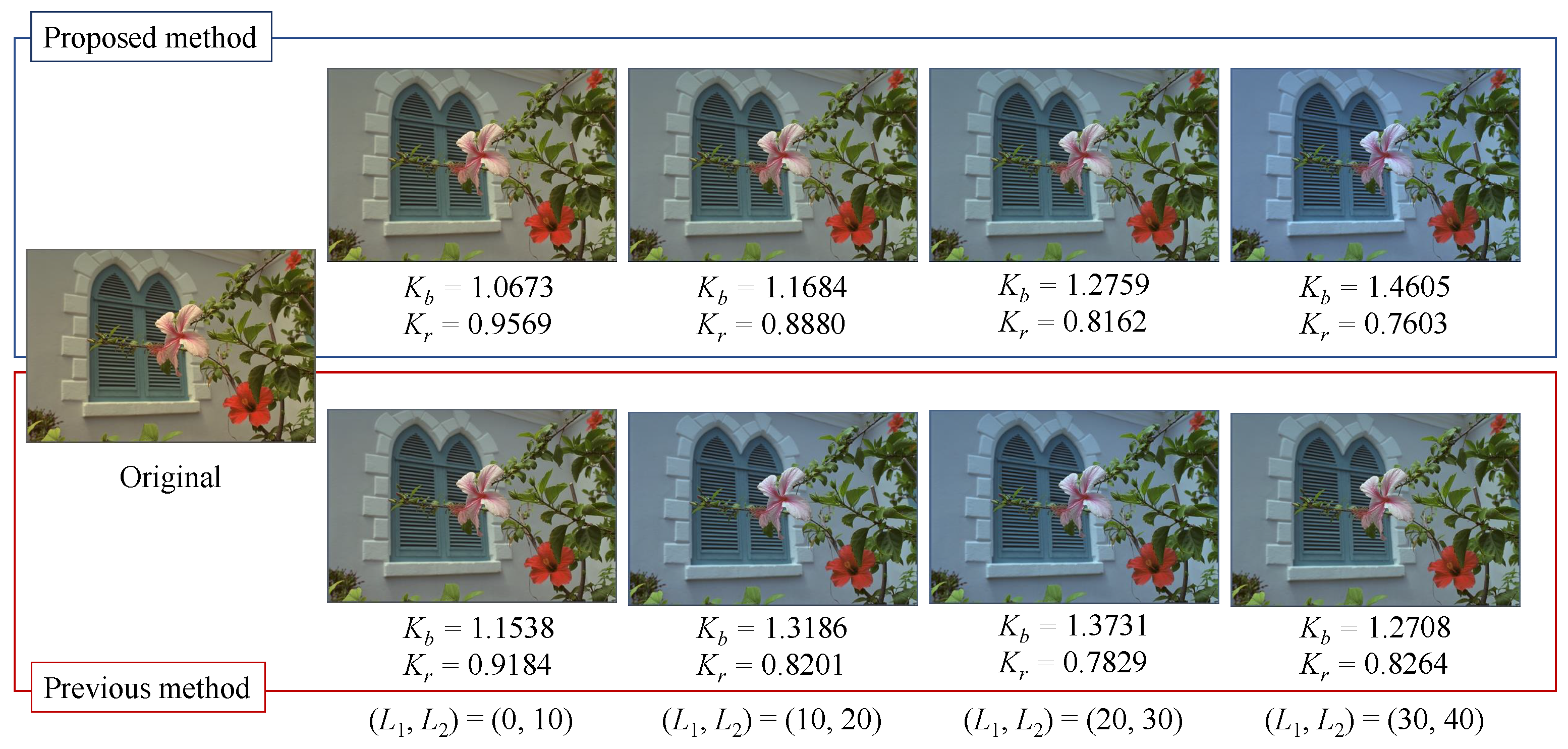
4.2. Color Tone Assessment of Output Images

Figure 8 shows the output images of kodim23 obtained by the proposed method. The upper and lower images show the results of the blue and red tone enhancement, respectively. As $L_1$ and $L_2$ were increased while retaining the dimension of the reference areas, the intensity of the enhancement improved. In this example, the intensity of the enhancement was at a maximum for $(L_1,L_2)=(30,40)$, and the output image was most effectively enhanced compared with the original image.

Figure 8. Output images (kodim23).

Table 2 shows the mean values of the correction coefficients calculated for each parameter. In this table, $K_b$ and $K_r$ are the correction coefficients for the blue and red tones, respectively. The blue tone was more effectively enhanced as $K_b$ became larger and $K_r$ became smaller, while the red tone was more effectively enhanced as $K_b$ became smaller and $K_r$ became larger. From this table, it is clear that the proposed method could gradually enhance the tones and had a wider range of enhancement. It should be noted that both methods could not derive the output images if there was no pixel in the reference areas. Nonetheless, for certain values of $L_1$ and $L_2$, the proposed method had a wider reference area than the previous method; thus, the number of images where the tone enhancement was effective with the proposed method was larger than that with the previous method.

Table 2. Mean values of correction coefficients for each parameter. Blue tone was more effectively enhanced as $K_b$ became larger and $K_r$ became smaller; in contrast, red tone was more effectively enhanced as $K_b$ became smaller and $K_r$ became larger.

	Blue Enhancement
	Proposed			Previous [18]
	$K_b$	$K_r$	Images with Effective	$K_b$	$K_r$	Images with Effective
			Tone Enhancement			Tone Enhancement
($L_1$, $L_2$) = (0, 10)	1.0554	0.9531	42	1.1544	0.9053	42
($L_1$, $L_2$) = (10, 20)	1.2061	0.8633	42	1.3307	0.8199	41
($L_1$, $L_2$) = (20, 30)	1.4190	0.7886	41	1.4828	0.7781	41
($L_1$, $L_2$) = (30, 40)	1.8299	0.7258	40	1.6471	0.7460	37
	Red Enhancement
	Proposed			Previous [18]
	$K_b$	$K_r$	Images with Effective	$K_b$	$K_r$	Images with Effective
			Tone Enhancement			Tone Enhancement
($L_1$, $L_2$) = (0, 10)	0.9611	1.0509	42	0.9142	1.1759	40
($L_1$, $L_2$) = (10, 20)	0.8693	1.1984	36	0.8588	1.2132	26
($L_1$, $L_2$) = (20, 30)	0.7898	1.4199	27	0.8057	1.3314	16
($L_1$, $L_2$) = (30, 40)	0.7289	1.7356	20	0.7657	1.4503	8

Figure 9 shows the results of the blue enhancement for kodim07.

Figure 9. Output images and correction coefficients for blue enhancement (kodim07).

The upper and lower images show the results obtained by using the proposed and previous methods, respectively. The intensity of the enhancement improved as $K_b$ became larger and $K_r$ became smaller. In the proposed method, the intensity of the enhancement gradually improved as the parameters were increased, and the intensity was at a maximum in the case of $(L_1,L_2)=(30,40)$. In comparison, in the previous method, the intensity was at a maximum in the case of $(L_1,L_2)=(20,30)$ and decreased at $(L_1,L_2)=(30,40)$. In addition, as mentioned above, the proposed method can control the intensity of the enhancement in a wider range than the previous method. For easy comparison, in this experiment, we generated output images by fixing the widths of the reference areas to 10 and shifting the positions of these areas. The sizes and positions of these areas can be flexibly defined depending on the user requirements for the intensity of enhancement. Consequently, the proposed method allows for more uniform and gradual enhancement compared with the previous method.

4.3. Influence of Output Image Quality on Data Embedding

For reversibility, we need to embed the recovery information into the intermediate images. The data-embedding process commonly causes distortion in the output image. We examined the influence of the data-embedding process on the output image quality. Table 3 summarizes the mean values of the PSNR and SSIM of the output images against the intermediate images.

Table 3. Quantitative assessment of output image quality.

	PSNR [dB]
	Blue Enhancement	Red Enhancement
($L_1$, $L_2$) = (0, 10)	53.78	52.38
($L_1$, $L_2$) = (10, 20)	48.42	46.17
($L_1$, $L_2$) = (20, 30)	45.31	41.65
($L_1$, $L_2$) = (30, 40)	42.63	38.27
	SSIM
	Blue Enhancement	Red Enhancement
($L_1$, $L_2$) = (0, 10)	0.9969	0.9952
($L_1$, $L_2$) = (10, 20)	0.9923	0.9868
($L_1$, $L_2$) = (20, 30)	0.9842	0.9646
($L_1$, $L_2$) = (30, 40)	0.9739	0.9276

From this table, it is clear that both the PSNR and SSIM values were generally high. It was also difficult to visually recognize any artifacts in the output images. In addition, Table 3 shows that the output image quality decreased as the intensity of the enhancement improved for both the blue and red enhancement. As the correction coefficients became larger, more pixels caused overflows, which is described in Section 3.1.2. In such a case, more recovery information was required and embedded into the intermediate image. This was the cause of the degradation in image quality. Nevertheless, the proposed method preserved the high quality of the output image, even in the case of $(L_1,L_2)=(30,40)$.

5. Conclusions

We propose an extension of the reversible tone enhancement method that allows for uniform control of the intensity of enhancement regardless of the image features. In the previous method, the intensity cannot be gradually enhanced in some cases. The proposed method has two main advantages in terms of overcoming the above issue. First, it can uniformly and gradually enhance the intensity by increasing the correction coefficients. We verified this advantage both objectively and quantitatively in experiments. Second, we can obtain the correction coefficients for blue and red tones separately, namely, the correction coefficients allow us to control the intensities of both the enhancement and suppression separately. Thus, we can not only enhance the R component but also suppress the B component overall for the red enhancement. In the same manner, we can not only enhance the B component but also suppress the R component overall for the blue enhancement. This results in a more effective tone enhancement in our method. We further ensure reversibility by embedding recovery information. Through our experiments, we clarified that the proposed method not only has the above advantages but also a wider range in terms of the intensity of enhancement compared with the previous method. We also proved that the data-embedding process for recovery information never seriously affected the output image quality, and the output images maintained high quality without any visible artifacts. In our future work, we will further expand the range of tone control.

References

- Farthan, A.R. Review on some methods used in image restoration. Int. Multidiscip. Res. J. 2020, 10, 13–16. [Google Scholar]
- Fayaz, S.; Parah, S.A.; Qureshi, G.J.; Kumar, V. Underwater image restoration: A state-of-the-art review. IET Image Process. 2021, 15, 269–285. [Google Scholar] [CrossRef]
- Su, J.; Xu, B.; Yin, H. A survey of deep learning approaches to image restoration. Neurocomputing 2022, 487, 46–65. [Google Scholar] [CrossRef]
- Ali, A.M.; Benjdira, B.; Koubaa, A.; El-Shafai, W.; Khan, Z.; Boulila, W. Vision transformers in image restoration: A survey. Sensors 2023, 23, 2385. [Google Scholar] [CrossRef] [PubMed]
- Wu, H.-T.; Dugelay, J.-L.; Shi, Y.-Q. Reversible image data hiding with contrast enhancement. IEEE Sig. Process. Lett. 2015, 22, 81–85. [Google Scholar] [CrossRef]
- Gao, G.; Shi, Y.-Q. Reversible data hiding using controlled contrast enhancement and integer wavelet transform. IEEE Sig. Process. Lett. 2015, 22, 2078–2082. [Google Scholar] [CrossRef]
- Chen, H.; Ni, J.; Hong, W.; Chen, T.-S. Reversible data hiding with contrast enhancement using adaptive histogram shifting and pixel value ordering. Sig. Process. Image Commun. 2016, 46, 1–16. [Google Scholar] [CrossRef]
- Wu, H.-T.; Tang, S.; Huang, J.; Shi, Y.-Q. A novel reversible data hiding method with image contrast enhancement. Sig. Process. Image Commun. 2018, 62, 64–73. [Google Scholar] [CrossRef]
- Wu, H.-T.; Mai, W.; Meng, S.; Cheung, Y.-M.; Tang, S. Reversible data hiding with image contrast enhancement based on two-dimensional histogram modification. IEEE Access 2019, 7, 83332–83342. [Google Scholar] [CrossRef]
- Wu, H.-T.; Huang, J.; Shi, Y.-Q. A reversible data hiding method with contrast enhancement for medical images. J. Vis. Commun. Image Represent. 2015, 31, 146–153. [Google Scholar] [CrossRef]
- Gao, G.; Wan, X.; Yao, S.; Cui, Z.; Zhou, C.; Sun, X. Reversible data hiding with contrast enhancement and tamper localization for medical images. Inf. Sci. 2017, 385–386, 250–265. [Google Scholar] [CrossRef]
- Kim, S.; Lussi, R.; Qu, X.; Huang, F.; Kim, H.J. Reversible data hiding with automatic brightness preserving contrast enhancement. IEEE Trans. Circuits Syst. Video Technol. 2019, 29, 2271–2284. [Google Scholar] [CrossRef]
- Shi, M.; Yang, Y.; Meng, J.; Zhang, W. Reversible data hiding with enhancing contrast and preserving brightness in medical image. J. Inform. Secur. Appl. 2022, 70, 103324. [Google Scholar] [CrossRef]
- Wu, H.-T.; Cao, X.; Jia, R.; Cheung, Y.-M. Reversible data hiding with brightness preserving contrast enhancement by two-dimensional histogram modification. IEEE Trans. Circuits Syst. Video Technol. 2022, 32, 7605–7617. [Google Scholar] [CrossRef]
- Wu, H.-T.; Wu, Y.; Guan, Z.; Cheung, Y.-M. Lossless contrast enhancement of color images with reversible data hiding. Entropy 2019, 21, 910. [Google Scholar] [CrossRef]
- Sugimoto, Y.; Imaizumi, S. An extension of reversible image enhancement processing for saturation and brightness contrast. J. Imaging 2022, 8, 27. [Google Scholar] [CrossRef] [PubMed]
- Sugimoto, Y.; Imaizumi, S. Reversible image processing for color images with flexible control. Appl. Sci. 2023, 13, 2297. [Google Scholar] [CrossRef]
- Nakaya, D.; Imaizumi, S. A reversible image processing method for color tone control using data hiding. In Proceedings of the APSIPA ASC, Taipei, Taiwan, 31 October–3 November 2023; pp. 599–604. [Google Scholar]
- Pasteau, F.; Strauss, C.; Babel, M.; Deforges, O.; Bedat, L. Improved colour decorrelation for lossless colour image compression using the LAR codec. In Proceedings of the European Signal Processing Conference, EUSIPCO 2009, Glasgow, Scotland, UK, 24–28 August 2009; pp. 2122–2126. [Google Scholar]
- International Standard ISO/IEC IS–15444–1; Information Technology—JPEG 2000 Image Coding System—Part 1: Core Coding System. 2019. Available online: https://www.iso.org/standard/78321.html (accessed on 15 May 2023).
- Howard, P.G.; Kossentini, F.; Martins, B.; Forchhammer, S.; Rucklidge, W.J. The emerging JBIG2 standard. IEEE Trans. Circuits Syst. Video Technol. 1998, 8, 838–848. [Google Scholar] [CrossRef]
- Motomura, R.; Imaizumi, S. A reversible data-hiding method with prediction-error expansion in compressible encrypted images. Appl. Sci. 2022, 12, 9418. [Google Scholar] [CrossRef]
- Available online: http://www.r0k.us/graphics/kodak/ (accessed on 15 May 2023).
- Zhang, L.; Wu, X.; Buades, A.; Li, X. Color demosaicking by local directional interpolation and non-local adaptive thresholding. J. Electron. Imaging 2011, 20, 023016. [Google Scholar]
Disclaimer/Publisher’s Note: The statements, opinions and data contained in all publications are solely those of the individual author(s) and contributor(s) and not of MDPI and/or the editor(s). MDPI and/or the editor(s) disclaim responsibility for any injury to people or property resulting from any ideas, methods, instructions or products referred to in the content. |
© 2024 by the authors. Licensee MDPI, Basel, Switzerland. This article is an open access article distributed under the terms and conditions of the Creative Commons Attribution (CC BY) license (https://creativecommons.org/licenses/by/4.0/).