Abstract
Driving experience and anticipatory driving are essential skills for humans to operate vehicles in complex environments. In the context of autonomous vehicles, the software must offer the related features of scenario understanding and motion prediction. The latter feature of motion prediction is extensively researched with several competing large datasets, and established methods provide promising results. However, the incorporation of scenario understanding has been sparsely investigated. It comprises two aspects. First, by means of scenario understanding, individual assumptions of an object’s behavior can be derived to adaptively predict its future motion. Second, scenario understanding enables the detection of challenging scenarios for autonomous vehicle software to prevent safety-critical situations. Therefore, we propose a method incorporating scenario understanding into the motion prediction task to improve adaptivity and avoid prediction failures. This is realized by an a priori evaluation of the scenario based on semantic information. The evaluation adaptively selects the most accurate prediction model but also recognizes if no model is capable of accurately predicting this scenario and high prediction errors are expected. The results on the comprehensive scenario library CommonRoad reveal a decrease in the Euclidean prediction error by % and a % reduction in mispredictions of our method compared to the benchmark model.
1. Introduction
Human driving skills depend on the driver’s experience [1]. The analysis by Rahman et al. [2] reveals that the lack of experience in interactive situations is the primary influence factor of fatal accidents. Moreover, the missing ability to recognize dangerous situations [3,4] and the higher likeliness for critical errors of inexperienced drivers [5,6] increase the risk of accidents. So, it becomes apparent that driving experience is essential to drive safely. Consequently, if we assume the human driver as the reference for an autonomous vehicle (AV) system, the question arises of how scenario understanding, the algorithmic equivalent of driving experience, can be integrated into the AV’s software to improve its safety, especially in interactive scenarios. The current state of the art focuses on motion prediction algorithms without explicitly considering scenario understanding to solve these interactive scenarios. There are several competitions on large datasets [7,8,9] to foster the development of motion prediction methods. Deep-learning algorithms with high accuracy regarding low average Euclidean error are currently at the top of the competition’s leaderboards. However, the leaderboards also reveal the high miss rate of these algorithms, which specifies the rate of erroneous predictions across all objects. Thus, there is a discrepancy in the state of the art that low mean prediction errors are achieved, but prediction failures with high maximum Euclidean errors can not be prevented. Furthermore, Schöller et al. [10] show that the accuracy of a prediction model depends on the object type and traffic scenario. Therefore, it is also desirable to adaptively select the model depending on the present scenario. These two points emphasize the need to incorporate scenario understanding into motion prediction to detect prediction failures a priori and to adaptively apply the prediction model for the respective scenario.
The presented research in this work addresses this need. Our proposed method, Self-Evaluation of Trajectory Predictors, is outlined in Figure 1. Depending on the semantic information, the method evaluates the current scenario in which the AV operates by means of scenario understanding. The evaluation output is either the selection of the most accurate valid trajectory prediction out of multiple available prediction models or the classification of the scenario as invalid. A scenario is classified as invalid if none of the given prediction models, the predictors, can output a trajectory with an error below a defined threshold of a specific metric. By this, safety-critical prediction scenarios with a high expected error are a priori detected. The method aims to imitate the human driving experience in terms of recognizing dangerous situations and adapting to scenarios. In summary, our main contributions are as follows:
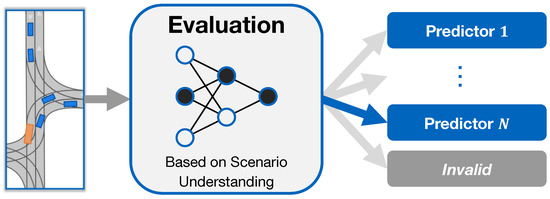
Figure 1.
Overview of the proposed method: self-evaluation of trajectory predictors for autonomous driving.
- A self-evaluation method for trajectory predictors, which adaptively selects the best prediction model for a present scenario or classifies the scenario invalid if no prediction model is suitable to avoid mispredictions.
- A hybrid prediction method consisting of three different prediction models, which are adaptively called by the algorithmic scenario understanding.
- A Proximity-Dependent Graph Neural Network for interaction-aware trajectory prediction.
The code used in this research is available as open-source software at https://github.com/TUMFTM/SETRIC (Initial Release, version 1.0.0) (14 February 2024).
2. Related Work
The following section reviews the broad field of motion prediction algorithms but focuses on prediction algorithms considering scenario understanding. The presented state of the art is then discussed to terminate the section.
Motion prediction algorithms can be divided into the three classes of physics-based, pattern-based, and planning-based approaches [11]. The most reputable motion prediction competitions [7,8,9] have been dominated by pattern-based approaches. Graph Neural Networks (GNNs) [12], especially transformer architectures or similar forms of attention mechanisms [13], are currently the most performant architectures because of their ability to model non-Euclidean interactions between road users, efficiently encode semantic information [14,15,16], or combine both tasks [17,18,19,20]. The prediction accuracy in these competitions is evaluated by mean Euclidean distance metrics such as the Root-Mean-Square Error (RMSE), the Average Displacement Error (ADE), and the Final Displacement Error (FDE). However, these metrics only reflect mean values and ignore outliers that could lead to safety-critical scenarios. However, there is still a considerable amount of outliers with high prediction errors, which is shown by the high miss rates of the prediction algorithms in the competitions. In the NuScenes prediction competition [8], the MissRate2k is defined as the proportion of mispredictions of all samples. If the maximum pointwise Euclidean distance between the prediction and ground truth is greater than 2 , a misprediction is given. For each object, the k most likely predictions are taken and evaluated to see if any of them are mispredictions. Due to the fact that the miss rate is not graded in the competition, the algorithms are not optimized to prevent mispredictions but instead only focus on the lowest mean distance error on the dataset. One approach to consider potential misprediction in the prediction output is the usage of uncertainty metrics. The Negative Log Likelihood (NLL) outputs the standard deviation to quantify the uncertainty of a trajectory [21,22,23]. In the case of maneuver predictions, the specification of probabilities [24] can be used. However, both approaches can not differentiate between the case of several possible options for the future motion or if the model can not understand the current scenario, which both lead to high uncertainty. In summary, none of the top-ranked models in the prediction competitions are able to prevent safety-critical mispredictions or to evaluate its own capability to accurately predict the future motion of surrounding objects in a scenario.
An approach that incorporates scenario understanding into motion prediction to improve adaptivity is presented by Ben-Younes et al. [25]. The authors introduce a method for context awareness by leveraging blind predictions, which aims to incorporate contextual information in addition to motion history. The model is trained using a training procedure designed to promote the use of semantic contextual cues. Two novel metrics, dispersion and convergence-to-range, are introduced to measure the temporal consistency of successive forecasts. The model outperforms previous works, as well as alternative de-biasing strategies. The results show that the method improves both the accuracy and stability of trajectory predictions compared to state-of-the-art methods. Novo et al. [26] propose a self-assessment framework for safety evaluation that focuses on prediction as a key component for safety. The concept involves three time constraints: a physical constraint based on the time required for emergency braking, a maneuver constraint based on the time needed to complete a driving maneuver, and a prediction model constraint based on the time horizon of a deep learning-based trajectory prediction model. The authors demonstrate the feasibility of the concept through specific use cases, such as lane changes in urban areas and on highways. Farid et al. [27] present a probabilistic run-time monitor that detects harmful prediction failures. The monitor uses trajectory prediction errors to reason about their impact on the AV and detects failures only if they are harmful to the AV’s safety. The results show that the monitor achieves the highest area under the receiver operating characteristic curve compared to the baseline methods, indicating its strong performance in detecting prediction failures. Carrasco et al. [28] propose a multi-modal motion prediction system that integrates evaluation criteria, robustness analysis, and interpretability of outputs. They analyze the limitations of current benchmarks and propose a new holistic evaluation framework that considers accuracy, diversity, and compliance with traffic rules. To enhance interpretability, they propose an intent prediction layer that clusters the output trajectories into high-level behaviors. The authors assess the effectiveness of their approach through a survey, confirming that multi-modal predictions and intention clustering improve the interpretability of the system’s output. The authors provide a comprehensive evaluation framework that considers both accuracy and interpretability. Shao et al. [29] argue that uncertainty estimation can be used to quantify the confidence of the model’s predictions and to detect potential failures. The proposed framework considers motion and model uncertainty and formulates various uncertainty scores for different prediction stages. The authors evaluate the approach using different prediction algorithms, uncertainty estimation methods, and uncertainty scores. The results show that uncertainty has potential for failure detection in motion prediction. Gomez-Huelamo et al. [30] propose a prediction method that combines deep learning with heuristic scenario understanding to achieve accurate trajectory forecasting. Attention mechanisms with GNNs are used to enhance the interactions among objects. The authors introduce heuristic proposals that provide preliminary plausible information about the future trajectories. These proposals consider the type of object and the scene geometry, such as lane distribution and possible goal points. The results of the experiments show that the proposed model achieves state-of-the-art performance with improved scenario understanding.
In the related field of human motion prediction, Fridovich-Keil et al. [31] introduce a confidence-aware method. The proposed method uses a Bayesian belief network to reason about the accuracy of a model’s predictions of human behavior. The authors demonstrate the effectiveness of their approach through experiments with a quadcopter navigating around a pedestrian. The results show that confidence-aware predictions lead to safer and more efficient motion planning than fixed confidence predictions. However, the approach is limited due to its computational complexity. Alternatively, social value orientation, which quantifies the ego objects’ rating of the surroundings’ welfare compared to their own, can be used to model interactions of pedestrians in a scenario [32]. The results show improved interaction behavior at pedestrian crossings but are limited in scaling the number of pedestrians. With a focus on object detection, Shao et al. [33] propose a framework called the Interpretable Sensor Fusion Transformer (InterFuser) for autonomous driving. The framework aims to address safety concerns and the lack of interpretability. It utilizes multi-modal multi-view sensors for comprehensive scenario understanding and adversarial event detection. The framework incorporates a transformer encoder to fuse information from different sensors and generate intermediate interpretable features. The AV’s actions are constrained by these features to safe sets. Extensive experiments on CARLA benchmarks [34] show that InterFuser outperforms prior methods and ranks first on the CARLA Leaderboard at the time of its publication. Focusing on the planned ego trajectory, a failure prediction is proposed by Kuhn et al. [35]. The authors also state that detecting critical traffic situations in advance is desirable to increase safety. The proposed approach uses machine learning to detect patterns in sequences of planned trajectories that indicate impending failures. The method is trained using data with disengagements by the safety driver. The results show that the proposed approach outperforms existing state-of-the-art failure prediction methods by more than 3% in terms of accuracy.
In summary, the presented state of the art in motion prediction is extensively investigated with prediction competitions on large-scale datasets. In contrast, the feature of scenario understanding is covered sparsely. The existing work that incorporates scenario understanding either uses overly conservative (physics-based) heuristics or focuses on the adaptability of the predicted trajectory but does not evaluate mispredictions. Other approaches need the ground truth for failure evaluation. None of the approaches combine multiple predictors into a hybrid module to adaptively output the best trajectory prediction. Our approach offers these features and provides an a priori evaluation based on comprehensive scenario understanding, which considers map information and object interaction. The evaluation either determines the best predictor from physics- and pattern-based prediction models for the respective scenario or classifies the scenario invalid if no model is suitable. By this, the evaluation improves the prediction accuracy and prevents safety-critical mispredictions. The hybrid prediction approach, which incorporates multiple methods and adaptively switches between them, is unique to the state of the art.
3. Method
In the following section, the architecture of the self-evaluation method is presented. In addition, the data processing and the training procedure are described. In the current implementation, illustrated in Figure 2, the self-evaluation method comprises Scene Image Encoding, three trajectory predictors (), and the Selector Model to evaluate the scenario, which are explained in detail below. The three trajectory predictors are as follows:
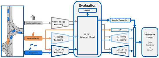
Figure 2.
The network architecture of the self-evaluation method for trajectory predictors comprises Scene Image Encoding, three trajectory predictors (CV, L_LSTM, DG_LSTM), and the Selector Model. Inputs are a rasterized image of the road network, the object’s history, and the surrounding objects’ states. All information is encoded and input into the evaluation. As a result of the evaluation, the Selector Model outputs the best trajectory predictor for the present scenario based on a specified metric. In the case that none of the predictors achieves the required accuracy, the prediction scenario is classified as invalid to avoid mispredictions.
- A Constant Velocity Model (CV)
- A Linear LSTM Model (L_LSTM)
- A Proximity-Dependent Graph–LSTM Model (DG_LSTM)
Thus, a physics-based model, a pattern-based linear model, and a pattern-based model with GNN-interaction representation are given. With this hybrid approach, a diverse range of scenarios and object behaviors can be accurately modeled. In general, the evaluation method can be built from various prediction models and is not limited to the presented implementation. This is beneficial to optimize the predictor selection for specific Operational Design Domains (ODDs), such as Highway scenarios (e.g., NGSIM [36]) with a high amount of constant velocity behavior or roundabout scenarios with a high amount of interactions (e.g., OpenDD [37]).
3.1. Scene Image Encoding
To enhance semantic understanding, a Scene Image Encoder is implemented, which is adapted from Geisslinger et al. [22]. Due to the vector representation of CommonRoad’s map, the road network is first processed into a rasterized scene image. The resulting image is of size with dedicated colors for the central lanes of the road network. The advantage of this representation is the independence from the road geometry and the number of roads since the input size remains unchanged compared to vector representations. For each object, the scene image is cut in a square around the object’s current position with a size of . The encoder comprises eight sequential convolutional neural network (CNN) layers with equal amounts of filters . Each layer halves the image dimensions, so an output array of size results, which ensures compatibility with the latent spaces of the LSTM encodings. As depicted in Figure 2, the encoded scene image is input to the Selector Model and to the decoders of the L_LSTM and DG_LSTM trajectory predictors. Thus, like the other encodings, the Scene Image Encoding is used multiple times to optimize the size of the network and to maximize the available information for the evaluation.
3.2. CV Model
In addition to the pattern-based models with Encoder–Decoder architectures, a CV-model, a physics-based approach, is incorporated into the self-evaluation method. It assumes that the object continues with constant speed and constant heading based on the current object’s state. Due to the transformation of the coordinate system in the data pre-processing step into the object’s view, the CV-prediction simplifies to
In the given equation, refers to the m-th predicted longitudinal position at the future time step within the prediction length . represents the current longitudinal speed of the object. The lateral future positions are zero because of the coordinate transformation. The output of the CV-model is the predicted trajectory of the object with its x-, y-positions over the prediction horizon of 5 . This output format applies to all prediction models to ensure consistency independent of the selected model. As inputs, only the object’s current position, orientation, and speed are considered. The CV-model does not require any training data and is computationally efficient. However, since it relies only on the current object state specified by the position, heading, and velocity, the model is sensitive to noise in these values. This makes the CV-model performance highly dependent on the upstream object tracking to reduce input noise. The model approach is chosen because of its high accuracy in the case of steady-state object behavior.
3.3. Linear LSTM Model
The L_LSTM-model consists of an LSTM-based single-layered Encoding with linear embedding and an LSTM-based Decoding (Figure 2). The encoder uses only the object’s history as input, so no interactions with other road users are considered. The L_LSTM-Encoding is input to both the Selector Model and to the L_LSTM-Decoding. The L_LSTM-Decoder is based on [38]. Compared to common LSTM-Decoders, temporal enrollment is realized by a direct expansion of the latent space up to the desired prediction length and one execution of the LSTM and not by iteratively calling the LSTM function up to the desired length. Experiments revealed an improved prediction accuracy of this approach. Even though the smoothness of the predicted trajectory deteriorates with this approach, it still stays around one magnitude below the displacement error. Thus, overall, the approach improves the prediction performance.
3.4. Proximity-Dependent Graph-LSTM Model
The DG_LSTM-model is constructed out of Proximity-Dependent GNN embedding and an LSTM-based encoder and decoder. The GNN embedding consisting of Graph Convolution (GC) layers models interactions between surrounding objects. For this purpose, the target object and its surrounding objects are processed into an undirected graph as input to the model. The objects are represented by the nodes , their interactions by the edges between the nodes. The objects’ states, namely their historical positions, angles, and class, are stored as node feature vectors z. Only interactions between traffic participants with a proximity of less than the threshold throughout the sampled historic and future time steps are considered. Hence, nodes of objects with greater Euclidean distances are not connected. A schematic depiction of this graph representation is shown in Figure 3.
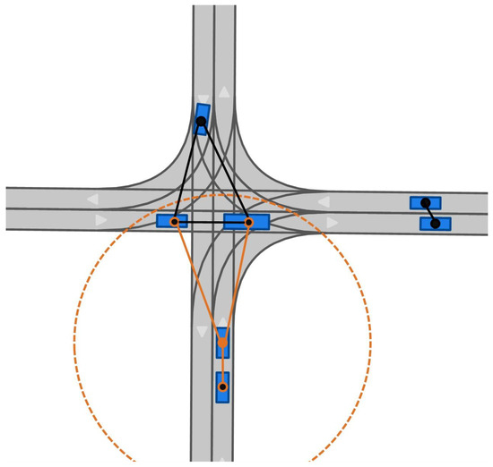
Figure 3.
Schematic depiction of the proximity-dependent graph representation for a traffic scenario. The orange circle represents the threshold , which filters the relevant objects (orange edges). Objects with a distance above the threshold are not connected to the target object (black edges).
The constructed undirected graph is input into the GC layers. Due to the fact that GC layers are more susceptible to vanishing gradients during backpropagation compared to classic convolution operations [39], the GNN embedding only stacks two GC layers. However, this still ensures interactions of second order. A single GC layer consists of three elementary steps that yield an updated embedding of all node feature vectors. In order to update the node feature vector of object i at time t, the following calculations are performed
At first, positions and angles of the connected surrounding objects j are transferred into the coordinate system of the target object i, which results in the modified feature vector . For subsequent GC layers, this coordinate transformation is not required because the node feature vectors are already embedded in a latent space. Next, the modified node feature vectors of the surrounding objects are processed via a common message function . Similarly, the node feature vector of the target object is processed by the message function . In our case, the message functions and are given by a linear-dense layer with subsequent ReLU activation. In the third step, the messages from all connected surrounding objects j, the output of , are aggregated via the function . These aggregated messages and the embedded node feature vector of the target object i are added element-wise and passed through an update function . Its output yields the final embedding as the new node feature vector of the target object i at time .
After the GNN embedding, the LSTM-Encoder is applied to incorporate temporal dependencies. Similar to the L_LSTM-model, a single-layered LSTM is utilized with an LSTM-cell number equivalent to the dimension of the embedded node feature vector. To output a trajectory prediction, the encoding is concatenated with the Scene Image Encoding and passed to the DG_LSTM-Decoding. By this, the DG_LSTM-model combines non-Euclidean interaction knowledge and rasterized road graph knowledge. The utilized decoder for this predictor has the same architecture as the L_LSTM-model and outputs the object’s future prediction by an LSTM layer. In addition, the DG_LSTM-Encoding is also input to the Selector Model.
3.5. Evaluation
The evaluation consists of the Selector Model G_SEL and a metric, which is needed to evaluate the predictors and to define invalid prediction scenarios. The inputs to the Selector Model are the three encodings of the scene image, L_LSTM, and DG_LSTM. These inputs are concatenated to a common latent space and passed through linear layers. The reuse of the three encodings has two advantages. First, the network size only grows by the selector head itself; no additional encoding is required for the evaluation, which enhances the efficiency of the architecture in terms of memory usage and inference time. Second, the selection model directly incorporates the knowledge of all predictors in a common latent space. The Selector Model’s output dimension is , which comprises the options to choose the best out of the three predictors or to classify a prediction scenario as invalid. The latter case applies if none of the predictors are expected to output a trajectory with a prediction error below a specified metric threshold. In the current implementation, the average RMSE over the prediction length is the used metric. The metric is defined over the prediction length between the predicted trajectory and ground truth for the prediction sample l as follows:
While the best prediction is defined by the lowest RMSE, classifying a scenario as invalid requires the specification of the error threshold . It can be set to a relative percentile of the RMSE distribution of the pre-trained predictors, or it can be set to an absolute RMSE value. In the first case, the percentile is created dynamically during the training process per batch. From an AV software engineer’s point of view, both options are useful. The option to set a percentile of a valid prediction can be used in unknown scenarios to ensure that the prediction output is optimized without knowing the absolute threshold value. In contrast, an absolute RMSE value as a threshold can be used during the tuning process of the ego-motion planner and the application of an AV software stack in a known ODD.
Since the model is executed in real-time, the metric is only used during training to determine the best predictor and to define invalid scenarios. During inference, the evaluation metric is unavailable because the model evaluates the scenarios a priori, and ground truth data can not be derived in real-time. Thus, the evaluation metric is learned by the model and is implicitly considered through the estimation of the best predictor during application.
The whole self-evaluation model is executed in stages during inference. First, the three encoders are executed to process the scenario. Next, the Selector Model is executed to determine the best predictor for the present scenario. Lastly, the output is generated. In the case that no predictor is suitable and the scenario is classified as invalid, none of the decoders are executed, and no trajectory is outputted. In the case that one of the predictors is selected, the respective model (CV) or decoder (L_LSTM, DG_LSTM) is executed, and the trajectory is outputted.
3.6. Data Processing
The used dataset is the scenario library of CommonRoad [40]. The library evaluates prediction and planning methods and consists of synthetic and real-world scenarios. There are, on average, objects per scenario, but half of the scenarios contain less or equal to 5 objects. Thus, it can be assumed that interactive multi-object scenarios and isolated scenarios with low interactions are represented. From the scenario library, 339,051 samples are extracted with 3 of object history and the road map as input, as well as 5 ground truth to be predicted. Both the history and ground truth future are sampled with 10 , which results in and of historical and future steps. Each sample also contains information about the surrounding objects to enable interaction awareness. The data processing transforms the target object’s past and surrounding object’s positions into the local coordinate system of the target object’s current pose. The transformation step results in a normalized input to the predictors, which improves the learning process.
3.7. Training and Optimization
Due to the integrative approach of the self-evaluation model with multiple concatenations between the different encodings and decodings, an adaption of the trainable parameters is required to train the respective predictors. This is realized by freezing network branches, while other branches are trained. Via this method, a specific optimization of the predictors is possible despite the nested model architecture. The Scene Image Encoding is always trained together with the first predictor. During the training of the other predictors, only the linear embedding at the output of the Scene Image Encoder, which connects the CNNs to the respective prediction decoder, is trained. The CNN layers remain frozen. The training order of the self-evaluation model starts with the L_LSTM. The DG_LSTM is trained afterward. This results in an advantage to the L_LSTM because the Scene Image Encoding is tailored to it. However, the DG_LSTM benefits less from the Scene Image Encoding due to the additional interaction knowledge from its GNN embedding, which explains why this order yields the optimal overall performance of both predictors. The predictors of L_LSTM and DG_LSTM are trained with the only goal of reducing their respective Euclidean prediction errors. So, their training processes do not consider the existence of the other predictors or the Selector Model. This choice is made because heterogeneous prediction behavior is expected from the different classes of predictors. On the same training data, it is expected that the respective predictors perform best in different scenario clusters because of the different modeling approaches. It would also be possible to train specialized predictors by splitting the data into clusters before the training. For example, the DG_LSTM-model could be trained only on scenarios with a high amount of traffic participants because it is expected to perform best in dense, interactive scenarios. The generalizability of the implementation also allows the choice of multiple identical models, which could be trained on isolated data clusters. The Selector Model is trained last to have access to all trained encoders. The encoders are frozen during the training, and only the Selector Model’s parameters are trained. For the training of the classification problem, the NLL-loss is used.
Large parts of the network architecture and hyperparameters are optimized by Bayesian Optimization [41]. The focus of the optimization is multi-modal. The optimization goal is a combination of the lowest overall RMSE of the model’s output and the best selection rate of the Selector Model. While a misselection between two approximately equally accurate predictors is acceptable because only a small increase in the prediction error is caused in the output, a misselection between two divergent predictors has a considerable impact on the output prediction error. So, both effects have to be considered in the optimization goal , which is defined as follows:
The equation shows the relation between the optimization goal , the selection rate of the Selector Model, and the of the model’s output. The minimal acceptable selection rate is empirically set to . The RMSE-threshold is set to . By means of these two variables, the optimization goals are balanced against each other. The optimization is conducted with a relative error threshold of the model’s output RMSE distribution to consider the dynamic improvement of the RMSE value during the optimization. After the optimization is finished, the RMSE-threshold for an invalid scenario is set to an absolute value of = for the validation on the test data, which is the 80% quantile of the best single predictor on the test data.
4. Results
In the following section, the performance of the self-evaluation method is validated on the CommonRoad dataset. The Wale-Net [22] serves as a benchmark model. Its base architecture [21] was, at the time of its release, in first place on the Argoverse dataset [7]. The model considers interactions between road users by Social Pooling and uses the same Scene Image Encoding as the self-evaluation model. It is re-trained on the same scenario split with the hyperparameters provided in Wale-Net’s open-source repository. In addition, the three individual predictors of the self-evaluation method are used for comparison to emphasize the effect of the combined hybrid evaluation model. Besides the analysis of the prediction error and the classification rate, analyses are conducted on the sensitivity of the Selector Model’s choices and on the actual improvement of the self-evaluation method compared to single predictors.
The RMSE over the prediction horizon of the self-evaluation method by means of the Selector Model G_SEL, compared to the single predictors and the benchmark model, is shown in Figure 4. The benchmark model is outperformed by both pattern-based predictors of the self-evaluation method. Only the physics-based CV-model shows a worse prediction behavior. It can be seen that the CV-model has a high accuracy on a short-term horizon up to but diverges with increasing prediction horizon. The L_LSTM-model performs best among the single predictors and also outperforms the DG_LSTM-model, even though it does not consider interactions between the surrounding objects. It can be interpreted that the dedicated training of the Scene Image Encoding in parallel to the L_LSTM outweighs the graph interaction knowledge of the DG_LSTM. In addition, the high ratio of highway scenarios in the CommonRoad dataset opts for a linear approach because of straight street geometry. The self-evaluation method, which combines the three predictors and additionally detects invalid predictions by means of the Selector Model G_SEL, outperforms all single predictors and achieves an average RMSE of . The FDE is reduced to compared to of the benchmark model. However, the ratio between the final and the mean RMSE is only improved to compared to the benchmark model’s ratio of . So, the progressive increase in the prediction error over the prediction horizon could not be mitigated.
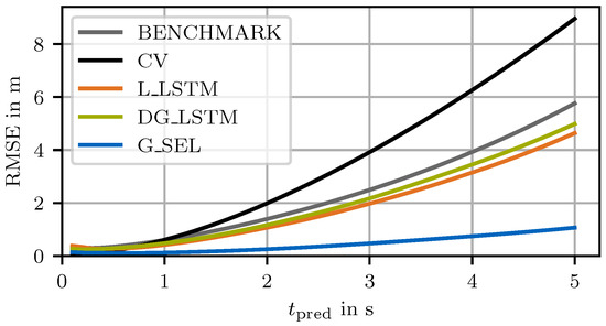
Figure 4.
RMSE over the prediction horizon of the benchmark model, the three single predictors (CV, L_LSTM, DG_LSTM), and the self-evaluation method by means of the Selector Model G_SEL. The error threshold for an invalid prediction is = .
To validate the self-evaluation method’s capability to avoid inaccurate predictions, the distribution of the RMSE is investigated (Figure 5). Like the RMSE over the prediction horizon, the benchmark model is already outperformed by the two single predictors. By means of the self-evaluation method, which additionally detects invalid predictions through the Selector Model G_SEL, the error distribution can be further reduced to a 90% quantile of , which is a reduction of % compared to the benchmark model. The reliability of the self-evaluation method is also validated by the MissRate21 (). The MissRate21 is reduced from the best single predictor, the L_LSTM, with % to % by the Selector Model. In comparison, the benchmark model’s MissRate21 is %. Thus, considering the scenario understanding induces an awareness of the model to detect predictions with high RMSE and avoids mispredictions.
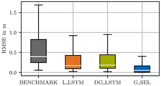
Figure 5.
Box of the mean RMSE over the prediction samples of the two best single predictors (L_LSTM, DG_LSTM) and the self-evaluation method by means of the Selector Model G_SEL compared the benchmark model ( = ). Box spans from the first to the third quartile. The median is shown in white. Whisker reach is .
Next, the Selector Model’s G_SEL classification performance is analyzed by the confusion matrix in Figure 6. The classes are given by the three predictors and the additional option of an invalid prediction. The Selector Model has to classify each scenario regarding the best predictor to use or, in case no model is suitable, to classify the scenario as invalid.
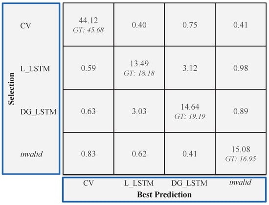
Figure 6.
Confusion matrix of the Selector Model ( = ). Ground truth in italic.
In total, = % correct selections are achieved. Compared to the ground truth, it can be seen that the G_SEL is limited in distinguishing between the L_LSTM and the DG_LSTM with over 3% wrong selections in both directions. It can be interpreted that the two pattern-based prediction models, despite the graph encoding, have a similar prediction behavior. The false positive rate, in the sense of valid predictions that are classified as invalid, is %. In contrast, the false negative rate for invalid predictions above the threshold that are classified as valid is %. It can be seen that the Selector Model has higher false negative rates towards the two pattern-based models compared to the CV-model. This can be explained by the fact that these two models are used to predict especially complex trajectories, which challenges the Selector Model to understand the scenario correctly and reliably select the invalid option. The tuning of the Selector Model towards specificity, i.e., a low false positive rate, is made because of the low overall RMSE threshold to avoid false positives with low RMSE and can be adjusted during the training process.
The discussed classification problem is an unambiguous task. However, the consequences of a misselection can greatly differ, depending on how big the deviation between the actual choice and the correct choice is. The analysis of this issue is important for the full stack applicability and to interpret the selection behavior of the model. Figure 7 shows the selection sensitivity between the valid predictors with varying tolerances for the correct selection. A tolerance of means that the selection is counted as correct if the RMSE error of the chosen predictor is ≤c% compared to the best predictor. The analysis is conducted over a range of error thresholds to also investigate the influence of the threshold. The analysis reveals that the selection rate increases by % on average over all thresholds when a tolerance of 5% is defined. Thus, the gap to 100% correct selections is dominated by unambiguous choices, i.e., a big deviation between the best prediction and the remaining predictors is given in the majority of the samples. This becomes even more obvious when the selection rate with is analyzed. The higher tolerance results in an increase in the selection rate by % compared to the baseline. So over 75% of the remaining wrong selections have a relative deviation of more than 10% between the best and the remaining predictors. This conclusion that the choices can be assumed unambiguous is also confirmed by the error distribution of the predictors on the test data. There is a mean difference of (standard deviation: ) between the best and second-best RMSE of the three predictors, which is an unambiguous difference compared to the mean RMSE (Figure 4). The presented evaluation in Figure 7 also shows the selection rate over the relative error threshold . It can be seen that the selection rate decreases from to . A small increase if all scenarios are defined valid can be observed. Thus, the model loses classification performance if the ratio of invalid predictions decreases. However, it has to be considered that the hyperparameter optimization is conducted with .
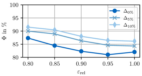
Figure 7.
Analysis of the selection sensitivity between the valid predictors with varying tolerances for the correct selection over the error threshold.
Lastly, the actual efficacy of the self-evaluation approach to improve the accuracy of the prediction output is analyzed in Figure 8. The RMSE of the self-evaluation method over varying error thresholds compared to an optimal selector, the best single predictor, and a random selector is shown. In comparison to the optimal selector (yellow), the self-evaluation method’s RMSE over the error thresholds (blue) is, on average, higher. For thresholds of and , the self-evaluation method is close to the optimal selector, but it loses performance for higher thresholds as already observed in the selection rate (Figure 7). Compared to the best single predictor (orange), the self-evaluation method improves the output RMSE even for a threshold of , i.e., without any invalid predictions. Thus, the hybrid approach is beneficial in any case. The comparison with a random selector (gray) shows that the self-evaluation method can correctly select the model with the lowest RMSE independent from the single predictors’ specification.
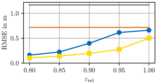
Figure 8.
Mean RMSE over the prediction samples for varying error thresholds of the self-evaluation method (blue) compared to an optimal selector (yellow) and a random selector (gray). In comparison, the best single predictor (orange) without self-evaluation is shown.
5. Discussion
A self-evaluation method for trajectory predictors for autonomous driving is presented and validated on the scenario library CommonRoad. The method incorporates scenario understanding, the equivalent of human driving experience, in the AV’s tasks of motion prediction to improve the overall prediction performance. This improvement is realized by an a priori scenario evaluation, which either selects the best trajectory prediction out of multiple models for the present scenario or, if none of the prediction models is expected to output an accurate prediction, reliably classifies the scenario as invalid to avoid mispredictions. The proposed self-evaluation method outperforms the benchmark and all single predictors in terms of average and final prediction error and reduces miss rate by %. This is achieved by a correct selection rate of % and a specificity of % of the Selector Model during the scenario evaluation. The confusion matrix presented indicates that the three predictors all have a relevant share of best predictions, confirming the advantage of the hybrid approach. The CV-model has the highest ratio of best predictions but also has the highest mean RMSE. It shows that constant velocity behavior is an accurate approach for simple steady-state scenarios but fails in more complex non-linear scenarios. The two pattern-based models achieve similar prediction accuracies. The influence of the map encoding can be seen in the L_LSTM-model, which is the best single predictor in total and even outperforms the interaction-aware Proximity-Dependent Graph-LSTM-model. The analysis of the selection sensitivity between the valid predictors shows that the selection of the correct predictor is an unambiguous task in the majority of the cases. Only a small improvement in the selection rate is achieved if the tolerance for a correct selection is increased. The analysis of the self-evaluation method’s impact on the overall RMSE reveals a nearly optimal selection behavior for error thresholds of and . It also reveals that even without the specification of invalid predictions, an improvement in the prediction accuracy is achieved. So, the hybrid prediction approach is beneficial in any case.
6. Conclusions
Regarding the intended usage of the self-evaluation prediction model in an AV stack, the following conclusions can be drawn. At first, the used predictors must be selected to cover the target ODD sufficiently. An essential constraint for choosing the predictors is the scene information provided by the predictors’ encoders to conduct the Selector Model. The presented implementation proposes three predictors with varying underlying assumptions. Variations in the used network architectures are possible for specific use cases. In the case of deep learning algorithms, it would also be possible to train specialized predictors on separated data clusters to ensure the coverage of the target ODD. Next, the Selector Model’s classification behavior, especially its specificity and sensitivity, and the error threshold must be tuned in combination with the respective ego-motion planner. For example, the false negative rate has to correlate with a more defensive behavior of the ego-motion planner to take account of the undetected invalid predictions. With the knowledge of the planning performance, an absolute error threshold to classify invalid predictions is recommended to ensure the required prediction accuracy to enable a safe ego-motion behavior and to base the planner parameterization on a shrunk prediction error window. It is important to mention that the invalid choice does not necessarily mean triggering an emergency state of the AV. With the a priori knowledge of an invalid prediction, the ego-motion planner can dynamically adjust its behavior to avoid dangerous situations. For example, an additional set of planner parameters can be deployed for the case of an invalid prediction scenario. The prediction module could switch to a shorter prediction horizon, or deterministic approaches such as the Reachable Sets [42] could be applied. Compared to the human driver, this adjustment of the motion prediction and planning corresponds to the natural reaction of decreasing speed and increasing the focus on the environment in unknown scenarios, which are not yet part of the individual driving experience.
Two open topics must be mentioned regarding the application in public road traffic. First, the definition of an invalid prediction, i.e., a prediction that is not manageable by the motion planner, highly depends on the particular scenario. In the presented work, we use the RMSE as a metric with an empirical threshold to define invalid predictions. It is assumed that a high RMSE of the predicted trajectory correlates with the criticality of a scenario. However, more comprehensive metrics are required to fully reflect a scenario’s criticality. Focusing just on the absolute prediction error does not cover the full scenario and does not entirely reveal its criticality. Second, even though the Selector Model achieves high correct selection rates, the safe application in AVs has to be analyzed. A reliable selection of the correct prediction or classification of a misprediction is essential to use this method in an AV stack. The full impact of a wrong selection on the AV behavior and the required safety features to handle these cases must be investigated. Furthermore, the necessary correct selection rate for a full-stack application has to be analyzed.
A possible future research direction to further adapt the self-evaluation method to human driving behavior is to not only detect the invalid scenarios but also to learn from them. One approach could be to store all scenarios that are initially classified as invalid and apply online learning to these scenarios. In the state of the art, self-supervised approaches for online learning [22,43,44] are presented to continuously improve a model and improve its generalizability. However, the major drawback to ensuring the stability of the model during the online learning process has to be considered. Despite that, the optimization of the Selector Model regarding robustness and selection rate, the analysis of the used metric, including the definition of invalid prediction scenarios, and the selection of the single prediction models are also future research directions.
Author Contributions
As the first author, P.K. initiated the idea of this paper and contributed essentially to its conception, implementation, and content. L.F. contributed to the conception, the implementation of the model and the writing of the paper. M.L. made an essential contribution to the conception of the research project. He revised the paper critically for important intellectual content. He gave final approval of the version to be published and agreed with all aspects of the work. As a guarantor, he accepts responsibility for the overall integrity of the paper. All authors have read and agreed to the published version of the manuscript.
Funding
This work was supported in part by the Bavarian Research Foundation through the project Data-Enabled Autonomous Driving and in part by the Institute for Automotive Technology through Basic Research Funds.
Institutional Review Board Statement
Not applicable.
Informed Consent Statement
Not applicable.
Data Availability Statement
The data used for this research are provided open source and are available at https://doi.org/10.5281/zenodo.8389720 (Access date on 1 February 2024).
Conflicts of Interest
The authors declare no conflicts of interest.
Abbreviations
The following abbreviations are used in this manuscript:
| ADE | Average Displacement Error |
| AV | Autonomous Vehicle |
| CNN | Convolutional Neural Network |
| CV | Constant Velocity Model |
| FDE | Final Displacement Error |
| DG_LSTM | Proximity-Dependent Graph-LSTM Model |
| GC | Graph Convolution |
| G_SEL | Selector Model |
| GNN | Graph Neural Network |
| L_LSTM | Linear LSTM Model |
| NLL | Negative Log Likelihood |
| ODD | Operational Design Domain |
| RMSE | Root-Mean-Square Error |
References
- Williams, A.F.; Carsten, O. Driver Age and Crash Involvement. Am. J. Public Health 1989, 79, 326–327. [Google Scholar] [CrossRef]
- Rahman, M.A.; Hossain, M.M.; Mitran, E.; Sun, X. Understanding the Contributing Factors to Young Driver Crashes: A Comparison of Crash Profiles of Three Age Groups. Transp. Eng. 2021, 5, 100076. [Google Scholar] [CrossRef]
- McKnight, A.; McKnight, A. Young Novice Drivers: Careless or Clueless? Accid. Anal. Prev. 2003, 35, 921–925. [Google Scholar] [CrossRef] [PubMed]
- Lee, S.E.; Klauer, S.G.; Olsen, E.C.B.; Simons-Morton, B.G.; Dingus, T.A.; Ramsey, D.J.; Ouimet, M.C. Detection of Road Hazards by Novice Teen and Experienced Adult Drivers. Transp. Res. Rec. 2008, 2078, 26–32. [Google Scholar] [CrossRef] [PubMed]
- McDonald, C.C.; Curry, A.E.; Kandadai, V.; Sommers, M.S.; Winston, F.K. Comparison of Teen and Adult Driver Crash Scenarios in a Nationally Representative Sample of Serious Crashes. Accid. Anal. Prev. 2014, 72, 302–308. [Google Scholar] [CrossRef] [PubMed]
- Seacrist, T.; Douglas, E.C.; Huang, E.; Megariotis, J.; Prabahar, A.; Kashem, A.; Elzarka, A.; Haber, L.; MacKinney, T.; Loeb, H. Analysis of Near Crashes among Teen, Young Adult, and Experienced Adult Drivers using the SHRP2 Naturalistic Driving Study. Traffic Inj. Prev. 2018, 19, 89–96. [Google Scholar] [CrossRef]
- Chang, M.F.; Lambert, J.; Sangkloy, P.; Singh, J.; Bak, S.; Hartnett, A.; Wang, D.; Carr, P.; Lucey, S.; Ramanan, D.; et al. Argoverse: 3D Tracking and Forecasting with Rich Maps. In Proceedings of the IEEE/CVF Conference on Computer Vision and Pattern Recognition (CVPR), Long Beach, CA, USA, 15–20 June 2019; pp. 8748–8757. [Google Scholar]
- Caesar, H.; Bankiti, V.; Lang, A.H.; Vora, S.; Liong, V.E.; Xu, Q.; Krishnan, A.; Pan, Y.; Baldan, G.; Beijbom, O. nuScenes: A Multimodal Dataset for Autonomous Driving. In Proceedings of the IEEE/CVF Conference on Computer Vision and Pattern Recognition (CVPR), Seattle, WA, USA, 13–19 June 2020; pp. 11621–11631. [Google Scholar]
- Ettinger, S.; Cheng, S.; Caine, B.; Liu, C.; Zhao, H.; Pradhan, S.; Chai, Y.; Sapp, B.; Qi, C.R.; Zhou, Y.; et al. Large Scale Interactive Motion Forecasting for Autonomous Driving: The Waymo Open Motion Dataset. In Proceedings of the IEEE/CVF International Conference on Computer Vision (ICCV), Montreal, BC, Canada, 11–17 October 2021; pp. 9710–9719. [Google Scholar]
- Schöller, C.; Aravantinos, V.; Lay, F.; Knoll, A. What the Constant Velocity Model Can Teach Us About Pedestrian Motion Prediction. IEEE Robot. Autom. Lett. 2020, 5, 1696–1703. [Google Scholar] [CrossRef]
- Karle, P.; Geisslinger, M.; Betz, J.; Lienkamp, M. Scenario Understanding and Motion Prediction for Autonomous Vehicles—Review and Comparison. IEEE Trans. Intell. Transp. Syst. 2022, 23, 16962–16982. [Google Scholar] [CrossRef]
- Wu, Z.; Pan, S.; Chen, F.; Long, G.; Zhang, C.; Yu, P.S. A Comprehensive Survey on Graph Neural Networks. IEEE Trans. Neural Netw. Learn. Syst. 2021, 32, 4–24. [Google Scholar] [CrossRef] [PubMed]
- Park, D.; Ryu, H.; Yang, Y.; Cho, J.; Kim, J.; Yoon, K.J. Leveraging Future Relationship Reasoning for Vehicle Trajectory Prediction. In Proceedings of the The Eleventh International Conference on Learning Representations, Kigali, Rwanda, 1–5 May 2023. [Google Scholar]
- Gilles, T.; Sabatini, S.; Tsishkou, D.; Stanciulescu, B.; Moutarde, F. GOHOME: Graph-Oriented Heatmap Output for future Motion Estimation. In Proceedings of the 2022 International Conference on Robotics and Automation (ICRA), Philadelphia, PA, USA, 23–27 May 2022; pp. 9107–9114. [Google Scholar] [CrossRef]
- Deo, N.; Wolff, E.; Beijbom, O. Multimodal Trajectory Prediction Conditioned on Lane-Graph Traversals. In Proceedings of the 5th Conference on Robot Learning, London, UK, 8–11 November 2022; Volume 164, pp. 203–212. [Google Scholar]
- Shi, S.; Jiang, L.; Dai, D.; Schiele, B. Motion Transformer with Global Intention Localization and Local Movement Refinement. Adv. Neural Inf. Process. Syst. 2022, 35, 6531–6543. [Google Scholar]
- Zeng, W.; Liang, M.; Liao, R.; Urtasun, R. LaneRCNN: Distributed Representations for Graph-Centric Motion Forecasting. In Proceedings of the 2021 IEEE/RSJ International Conference on Intelligent Robots and Systems (IROS), Prague, Czech Republic, 27 September–1 October 2021; pp. 532–539. [Google Scholar] [CrossRef]
- Gilles, T.; Sabatini, S.; Tsishkou, D.; Stanciulescu, B.; Moutarde, F. THOMAS: Trajectory Heatmap Output with learned Multi-Agent Sampling. In Proceedings of the International Conference on Learning Representations, Online, 25–29 April 2022. [Google Scholar]
- Varadarajan, B.; Hefny, A.; Srivastava, A.; Refaat, K.S.; Nayakanti, N.; Cornman, A.; Chen, K.; Douillard, B.; Lam, C.P.; Anguelov, D.; et al. MultiPath++: Efficient Information Fusion and Trajectory Aggregation for Behavior Prediction. In Proceedings of the 2022 International Conference on Robotics and Automation (ICRA), Philadelphia, PA, USA, 23–27 May 2022; pp. 7814–7821. [Google Scholar] [CrossRef]
- Wirth, F.J. Conditional Behavior Prediction of Interacting Agents on Map Graphs with Neural Networks. Ph.D. Thesis, Karlsruher Institut für Technologie (KIT), Karlsruhe, Germany, 2023. [Google Scholar] [CrossRef]
- Deo, N.; Trivedi, M.M. Convolutional Social Pooling for Vehicle Trajectory Prediction. In Proceedings of the IEEE Conference on Computer Vision and Pattern Recognition (CVPR) Workshops, Salt Lake City, UT, USA, 18–23 June 2018; pp. 1468–1476. [Google Scholar]
- Geisslinger, M.; Karle, P.; Betz, J.; Lienkamp, M. Watch-and-Learn-Net: Self-supervised Online Learning for Probabilistic Vehicle Trajectory Prediction. In Proceedings of the 2021 IEEE International Conference on Systems, Man, and Cybernetics (SMC), Prague, Czech Republic, 9 October 2021; pp. 869–875. [Google Scholar] [CrossRef]
- Mozaffari, S.; Sormoli, M.A.; Koufos, K.; Dianati, M. Multimodal Manoeuvre and Trajectory Prediction for Automated Driving on Highways Using Transformer Networks. IEEE Robot. Autom. Lett. 2023, 8, 6123–6130. [Google Scholar] [CrossRef]
- Gomes, I.P.; Premebida, C.; Wolf, D.F. Interaction-aware Maneuver Prediction for Autonomous Vehicles using Interaction Graphs. In Proceedings of the 2023 IEEE Intelligent Vehicles Symposium (IV), Anchorage, AL, USA, 4–7 June 2023; pp. 1–8. [Google Scholar] [CrossRef]
- Ben-Younes, H.; Zablocki, E.; Chen, M.; Pérez, P.; Cord, M. Raising Context Awareness in Motion Forecasting. In Proceedings of the IEEE/CVF Conference on Computer Vision and Pattern Recognition (CVPR) Workshops, New Orleans, LO, USA, 18–24 June 2022; pp. 4409–4418. [Google Scholar]
- Stockem Novo, A.; Hürten, C.; Baumann, R.; Sieberg, P. Self-evaluation of Automated Vehicles based on Physics, State-of-the-Art Motion Prediction and User Experience. Sci. Rep. 2023, 13, 12692. [Google Scholar] [CrossRef] [PubMed]
- Farid, A.; Veer, S.; Ivanovic, B.; Leung, K.; Pavone, M. Task-Relevant Failure Detection for Trajectory Predictors in Autonomous Vehicles. In Proceedings of the 6th Conference on Robot Learning, Atlanta, GA, USA, 6–9 November 2023; Volume 205, pp. 1959–1969. [Google Scholar]
- Carrasco Limeros, S.; Majchrowska, S.; Johnander, J.; Petersson, C.; Sotelo, M.Ä.; Fernández Llorca, D. Towards trustworthy multi-modal motion prediction: Holistic evaluation and interpretability of outputs. CAAI Trans. Intell. Technol. 2023. [CrossRef]
- Shao, W.; Xu, Y.; Peng, L.; Li, J.; Wang, H. Failure Detection for Motion Prediction of Autonomous Driving: An Uncertainty Perspective. arXiv 2023, arXiv:2301.04421. [Google Scholar]
- Gómez-Huélamo, C.; Conde, M.V.; Barea, R.; Bergasa, L.M. Improving Multi-Agent Motion Prediction with Heuristic Goals and Motion Refinement. In Proceedings of the IEEE/CVF Conference on Computer Vision and Pattern Recognition (CVPR) Workshops, Vancouver, BC, Canada, 17–24 June 2023; pp. 5322–5331. [Google Scholar]
- Fridovich-Keil, D.; Bajcsy, A.; Fisac, J.F.; Herbert, S.L.; Wang, S.; Dragan, A.D.; Tomlin, C.J. Confidence-aware Motion Prediction for Real-time Collision Avoidance. Int. J. Robot. Res. 2020, 39, 250–265. [Google Scholar] [CrossRef]
- Crosato, L.; Shum, H.P.H.; Ho, E.S.L.; Wei, C. Interaction-Aware Decision-Making for Automated Vehicles Using Social Value Orientation. IEEE Trans. Intell. Veh. 2023, 8, 1339–1349. [Google Scholar] [CrossRef]
- Shao, H.; Wang, L.; Chen, R.; Li, H.; Liu, Y. Safety-Enhanced Autonomous Driving Using Interpretable Sensor Fusion Transformer. In Proceedings of the 6th Conference on Robot Learning, Atlanta, GA, USA, 6–9 November 2023; Volume 205, pp. 726–737. [Google Scholar]
- Dosovitskiy, A.; Ros, G.; Codevilla, F.; Lopez, A.; Koltun, V. CARLA: An Open Urban Driving Simulator. In Proceedings of the 1st Annual Conference on Robot Learning, Mountain View, CA, USA, 13–15 November 2017; Volume 78, pp. 1–16. [Google Scholar]
- Kuhn, C.B.; Hofbauer, M.; Petrovic, G.; Steinbach, E. Trajectory-Based Failure Prediction for Autonomous Driving. In Proceedings of the 2021 IEEE Intelligent Vehicles Symposium (IV), Nagoya, Japan, 11–17 July 2021; pp. 980–986. [Google Scholar] [CrossRef]
- Colyar, J.; Halskias, J. US Highway 101 Dataset; Office of Safety Research and Development: Washington, DC, USA, 2007. Available online: https://www.fhwa.dot.gov/publications/research/operations/07030/ (accessed on 1 February 2024).
- Breuer, A.; Termöhlen, J.A.; Homoceanu, S.; Fingscheidt, T. openDD: A Large-Scale Roundabout Drone Dataset. In Proceedings of the 2020 IEEE 23rd International Conference on Intelligent Transportation Systems (ITSC), Rhodes, Greece, 20–23 September 2020; pp. 1–6. [Google Scholar] [CrossRef]
- Karle, P.; Török, F.; Geisslinger, M.; Lienkamp, M. MixNet: Physics Constrained Deep Neural Motion Prediction for Autonomous Racing. IEEE Access 2023, 11, 85914–85926. [Google Scholar] [CrossRef]
- Li, G.; Muller, M.; Thabet, A.; Ghanem, B. DeepGCNs: Can GCNs Go As Deep As CNNs? In Proceedings of the IEEE/CVF International Conference on Computer Vision (ICCV), Seoul, Republic of Korea, 27 October–2 November 2019. [Google Scholar]
- Althoff, M.; Koschi, M.; Manzinger, S. CommonRoad: Composable benchmarks for motion planning on roads. In Proceedings of the 2017 IEEE Intelligent Vehicles Symposium (IV), Los Angeles, CA, USA, 22–29 October 2017; pp. 719–726. [Google Scholar] [CrossRef]
- Snoek, J.; Larochelle, H.; Adams, R.P. Practical Bayesian Optimization of Machine Learning Algorithms. Adv. Neural Inf. Process. Syst. 2012, 25. [Google Scholar]
- Althoff, M.; Dolan, J.M. Online Verification of Automated Road Vehicles Using Reachability Analysis. IEEE Trans. Robot. 2014, 30, 903–918. [Google Scholar] [CrossRef]
- Hao, C.; Chen, Y.; Cheng, S.; Zhang, H. Improving Vehicle Trajectory Prediction with Online Learning. In Proceedings of the 2023 IEEE Intelligent Vehicles Symposium (IV), Anchorage, AL, USA, 4–7 June 2023; pp. 1–7. [Google Scholar] [CrossRef]
- Janjos, F.; Keller, M.; Dolgov, M.; Zöllner, J.M. Bridging the Gap Between Multi-Step and One-Shot Trajectory Prediction via Self-Supervision. In Proceedings of the 2023 IEEE Intelligent Vehicles Symposium (IV), Anchorage, AL, USA, 4–7 June 2023; pp. 1–8. [Google Scholar]
Disclaimer/Publisher’s Note: The statements, opinions and data contained in all publications are solely those of the individual author(s) and contributor(s) and not of MDPI and/or the editor(s). MDPI and/or the editor(s) disclaim responsibility for any injury to people or property resulting from any ideas, methods, instructions or products referred to in the content. |
© 2024 by the authors. Licensee MDPI, Basel, Switzerland. This article is an open access article distributed under the terms and conditions of the Creative Commons Attribution (CC BY) license (https://creativecommons.org/licenses/by/4.0/).