Position–Force Control of a Lower-Limb Rehabilitation Robot Using a Force Feed-Forward and Compensative Gravity Proportional Derivative Method

Abstract

The design and control of lower-limb rehabilitation robots for patients after a stroke has gained significant attention. This paper presents the dynamic analysis and control of a 3-degrees-of-freedom lower-limb rehabilitation robot using combined position–force control based on the force feed-forward and compensative gravity proportional derivative methods. In the lower-limb rehabilitation robot, the interaction force between the patient with the joints and links of the robot is uncertain and nonlinear due to the disturbance effect of Coriolis force, centrifugal force, gravitational force, and friction force. During recovery stages, the forces exerted by the patient’s lower limbs are also considered disturbances. Therefore, to meet the quality requirements in using the rehabilitation robot with different recovery stages of patient training, combining position control and force control is essential. In this paper, we proposed a combination of proportional–derivative gravity compensation motion control and force feed-forward control to form an advanced combined controller (position–force feed-forward control—PFFC) for a 3 DOF lower-limb functional rehabilitation robot. The forces can be sensed using a 3-axis force sensor. In addition, the robot’s position parameters are also measured by encoders. The control algorithm is implemented on the STM32F4 Discovery board. A verified test of the proposed control method is shown in the experiments, showing the good performance of the system.

1. Introduction

It is common for patients after a stroke to develop a disability related to lower-limb movement. A movement disability of the lower limbs is the biggest obstacle in the patient’s daily life [1]. Researching and developing exercise methods to support post-stroke patients in improving lower-limb rehabilitation is an important task [2,3]. Many studies have indicated that the movement disabilities of post-stroke patients can be enhanced through pre-designed recovery programs involving high-intensity therapy methods and repeating exercises [4,5,6,7]. Previous studies also show that robot-assisted lower-limb rehabilitation and therapist-guided rehabilitation programs are equally effective [8]. Moreover, robots can systematically assist patients in recovering through pre-programmed rehabilitation exercises. Applying robots to rehabilitation helps to evaluate patients’ recovery status by analyzing the data recorded in the robotic training process [9,10,11,12,13]. The research and development of rehabilitation robots is a field of study that is gaining attention from many researchers [14,15,16,17,18,19,20,21,22,23,24]. The objective of rehabilitation for stroke patients is to increase muscle strength, endurance, and mobility through repetitive movements until the trajectory and angle of joints are enhanced or maintained. The rehabilitation process for patients after a stroke can be divided into three stages, including an early recovery stage, an intermediate stage, and an advanced recovery stage. In the early recovery stage, following repetitive passive exercises along predetermined trajectories, the patient’s limb movement ability and muscle strength may partially recover. In this stage, position controllers are used to control the operation of the rehabilitation robot. Nevertheless, upon entering the intermediate stage of recovery, the position controller may diminish the patients’ active and proactive exercising efforts. Therefore, a force control method to create interaction between the patient and the robot is necessary at this stage.

From the previous research shown in ref [17], the pure PID controller works well when the system is represented as a mathematical model without uncertainties and disturbances. Previous studies [22] have also shown that the compensative gravity PD controller works better than the pure PID controller when we consider the effect of the robot’s gravity itself as a source of disturbance. However, both pure PID and the compensative gravity PD controller can not cope with a change in the forces impacting the system.

To appropriately address the force interaction effect between humans and robots, a force-feedback controller needs to be integrated into the robot. The force-feedback controller aids in replicating forces based on the user’s actions, facilitating the perception of the robot’s force during control operations [20]. The force-feedback system with force sensors and rotary encoders can measure the force and rotation angle of the joints. Then, the measured force is fed back to the controller so that the robot can sense the interaction force and assist patients. Force-feedback control has many advantages and has been extensively studied for upper-limb exoskeletons [25]. These studies have improved control performance significantly, and are demonstrated by simulation and experiment results [25,26,27,28,29]. In lower-limb rehabilitation robots, force-feedback controllers have also been studied and developed in several authors. In [26], an exoskeleton has six flexible force sensors placed on the sole of the shoe, and two force sensors attached between the distal end of the shank and the ankle joint. Force-feedback control is performed by comparing the ground reaction force with the force of the hydraulic cylinder to promote the user’s interaction force. A research group at the Institute of Mechanics—Vietnam Academy of Science and Technology proposes a force control method using a force feed-forward control model [20,22]. The proposed control method controls the torque of an upper-limb exoskeleton and controls a lower-limb rehabilitation robot. The simulation and experimental results showed that with this controller, both upper-limb and lower-limb robots can sense the forces exerted by the user, and the controller can generate control forces to compensate for the previously applied user forces. The force feed-forward controller computes and generates control torques to counteract the interaction forces induced by the therapist to aid patients in performing exercises.

However, during the early training stage, focusing on position control, forces exerted by the patient’s lower limbs are considered disturbances. Therefore, to meet the flexibility requirements in using the rehabilitation robot with different stages of patient training, combining position control and force control is essential. Furthermore, from a control perspective, in the case of the 3-degrees-of-freedom (DOF) lower-limb rehabilitation robot, the robot and the user are two independent systems interacting through forces. These interaction forces affect both the robot and the user according to Newton’s third law, and depend on the control methods used to control the robot. Therefore, for the system to be well controlled in terms of force, a control method resilient to disturbances and interaction force-feedback control seems capable of meeting these requirements. A primary concern in research on rehabilitation robot control is providing appropriate assistance to patients to perform exercises suitable for each stage of recovery. With the above reasons, the authors proposed a combination of proportional–derivative gravity compensation motion control and force feed-forward control to form an advanced combined controller (position–force feed-forward control—PFFC) for a 3 DOF lower-limb functional rehabilitation robot.

This paper presents the results of research on position–force control for a 3 DOF lower-limb rehabilitation robot using a combined force feed-forward and gravity compensation proportional–derivative control method. The paper is structured as follows: Section 2 describes the mathematical model of the robot. Section 3 proposes and applies the combination of position and force control to the 3 DOF lower-limb rehabilitation robot. Finally, Section 4 describes the experiment results to verify the performance of the proposed control method.

2. Mathematical Model

2.1. Robot’s Structure

This section describes a 3 DOF lower-limb rehabilitation robot designed to assist with patient recovery. The robot comprises three main joints corresponding to the hip, knee, and ankle. These joints are connected by a series of links: a base link, thigh link, leg link, and foot platform. Geared DC motors provide actuation for each joint. Figure 1 presents a schematic diagram of the 3 DOF rehabilitation robot. A Cartesian coordinate system is assigned to each link of the robot. Since all joint axes are parallel, twist angles (α_i) and translational distances (d_i) are considered negligible. To facilitate force control using a force feed-forward control model, geared DC motors with encoders are incorporated at each joint. Encoders provide joint-angle measurements, while force sensors measure the forces applied either by therapists during training stages or by the user’s foot during practice stages.

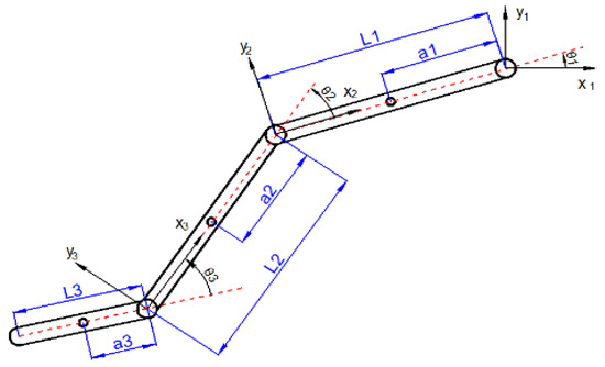
Figure 1. The schematic diagram of the 3 DOF rehabilitation robot.

2.2. Kinematic Model

Table 1 shows the Denavite–Hartenberge (D-H) parameters of the robot, where the parameters a_i are constant, and only the variables θ_i vary by rotation around z_i axis.

Table 1. D-H parameter of the lower-limb rehabilitation robot.

Joint i	αi Parameter	ai Parameter	di Parameter	θi Parameter
1st joint	0	l1	0	θ1
2nd joint	0	l2	0	θ2
3rd joint	0	l3	0	θ3

Using Equations (1) and (2), transformation matrices are established [30].

$${}^{i-1}A_i=\left[\begin{array}{cccc}\cos {\theta }_i& -\sin {\theta }_i\cos {\alpha }_i& \sin {\theta }_i\sin {\alpha }_i& a_i\cos {\theta }_i\\ \sin {\theta }_i& \cos {\theta }_i\cos {\alpha }_i& -\cos {\theta }_i\sin {\alpha }_i& a_i\sin {\theta }_i\\ 0& \sin {\alpha }_i& \cos {\alpha }_i& d_i\\ 0& 0& 0& 1\end{array}\right]$$

(1)

$$A_i={}^{0}A_1{}^{1}A_2\dots {}^{i-1}Ai$$

(2)

We have the following transformation matrices:

$$\begin{gathered} A_1=\left[\begin{array}{cccc}cos{\mathsf{\theta }}_1& -sin{\mathsf{\theta }}_1& 0& l_{1}cos{\mathsf{\theta }}_1\\ sin{\mathsf{\theta }}_1& cos{\mathsf{\theta }}_1& 0& l_{1}sin{\mathsf{\theta }}_1\\ 0& 0& 1& 0\\ 0& 0& 0& 1\end{array}\right] \\ {A}_2=\left[\begin{array}{cccc}cos{\mathsf{\theta }}_{12}& -sin{\mathsf{\theta }}_{12}& 0& l_{1}cos{\mathsf{\theta }}_1+l_{2}cos{\mathsf{\theta }}_{12}\\ sin{\mathsf{\theta }}_{12}& cos{\mathsf{\theta }}_{12}& 0& l_{1}sin{\mathsf{\theta }}_1+l_{2}sin{\mathsf{\theta }}_{12}\\ 0& 0& 1& 0\\ 0& 0& 0& 1\end{array}\right] \\ {A}_3=\left[\begin{array}{cccc}\cos {\theta }_{123}& -\sin {\theta }_{123}& 0& l_1\cos {\theta }_1+l_2\cos {\theta }_{12}+l_3\cos {\theta }_{123}\\ \sin {\theta }_{123}& \cos {\theta }_{123}& 0& l_1\sin {\theta }_1+l_2\sin {\theta }_{12}+l_3\sin {\theta }_{123}\\ 0& 0& 1& 0\\ 0& 0& 0& 1\end{array}\right] \end{gathered}$$

(3)

where ${\theta }_{12}={\theta }_1+{\theta }_2$, ${\theta }_{123}={\theta }_1+{\theta }_2+{\theta }_3$.

From Equation (3), we can obtain the direct kinematic model and the inverse kinematic model of the robot.

2.3. Dynamic Model

The robot’s dynamic model is written in matrix form as:

$$\mathit{M}\left(q\right)\ddot{q}+\mathit{C}(q,\dot{q})\dot{q}+\mathit{G}\left(q\right)=\tau$$

(4)

where

• $\mathit{M}(q)=\left[\begin{array}{ccc}{m}_{11}& m_{12}& m_{13}\\ m_{21}& m_{22}& m_{23}\\ m_{31}& m_{32}& m_{11}\end{array}\right]$ is the manipulator inertia matrix,
• $\mathit{C}\left(q,\dot{q}\right)\dot{q}=\left[\begin{array}{ccc}{c}_{11}& c_{12}& c_{13}\\ c_{21}& c_{22}& c_{23}\\ c_{31}& c_{32}& c_{11}\end{array}\right]$ is centrifugal and Coriolis matrix,
• $\mathit{G}\left(q\right)={\left[\begin{array}{ccc}{G}_1& G_2& G_2\end{array}\right]}^T$ is the gravitational vector,
• $q={\left[\begin{array}{ccc}{\theta }_1& {\theta }_2& {\theta }_3\end{array}\right]}^T$ is the vector of generalized Lagrange coordinates,
• $\tau ={\left[\begin{array}{ccc}{\tau }_1& {\tau }_2& {\tau }_2\end{array}\right]}^T$ is the vector of generalized forces.

Calculating and substituting matrices M, C, and vector G into Equation (4), three dynamical equations of motion ${\tau }_1,{\tau }_2,{\tau }_3$ are calculated.

3. Position–Force Control Using Force Feed-Forward and Compensative Gravity Proportional Derivative Method

3.1. The Structure Diagram of the Controller

The PFFC controller has two tasks: trajectory tracking and force control. The controller will set an initial torque and maintain the torque to control the joints with the design trajectory. There are two phases to perform this task. In the first stage, the therapist applies force to the robot’s links and moves it along the joint-angle trajectory corresponding to the rehabilitation exercise. Rehabilitation exercises will depend on each stage of the process. The force exerted by the therapist on the robot is measured by force sensors. The joint angles are measured by encoders located at joints. The force and joint angles will be recorded by the software and displayed on the user interface of the computer. In the second phase, the joint trajectories measured in the initial phase are set in the position controller as setpoint signals, and the controller will control the robot’s motion to follow these trajectories. During operation, the force controller will generate control forces corresponding to the therapist’s force to control the joints. At the same time, the force sensor will measure the force exerted by the patient’s lower limb and feedback to the input of the controller. The forces and motion trajectories of the joints are continuously measured, recorded, and displayed by the software on the computer user interface, enabling therapists to monitor the patient’s training parameters. The proposed structure diagram of the PFFC is shown in Figure 2.

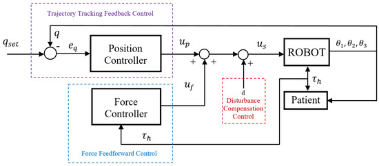
Figure 2. The structure diagram of the controller.

The proposed controller includes two control loops. The first loop is trajectory tracking feedback control. The joint-angle values ${\theta }_1, {\theta }_2, {\theta }_3$ of the hip, knee, and ankle joints are measured by the encoders and compared with the design trajectory value, ${\mathit{q}}_{\mathit{s}\mathit{e}\mathit{t}}={\left({\theta }_{set1}, {\theta }_{set2}, {\theta }_{set3}\right)}^T$. The error between the measured value and the design value is sent to the input of the position controller, with the output denoted as ${\mathit{u}}_{\mathit{p}}$. The design trajectory ${\mathit{q}}_{\mathit{s}\mathit{e}\mathit{t}}$ is obtained from the training process of the robot. The second loop is the force control. The force control method used the force feed-forward control model. The ${\mathit{\tau }}_{\mathit{h}}$ is torque obtained from measuring the force exerted between the robot and the patient by sensors. The interaction torque, ${\mathit{\tau }}_{\mathit{h}}$, is fed into the input of the force controller, and the output of this controller is denoted as ${\mathit{u}}_{\mathit{f}}$. The disturbance control is used to compensate for the friction and damping of the system.

3.2. Control Method

3.2.1. Trajectory Tracking Feedback Control

The position controller is chosen below:

$${\mathit{\tau }}_{\mathrm{đ}k}=\mathit{G}\left(q\right)+{\mathit{K}}_{p}e-{\mathit{K}}_d\dot{\mathit{q}}$$

(5)

where

$\mathit{G}\left(q\right)$—gravity compensation part;

${\mathit{K}}_{\mathit{p}}e-{\mathit{K}}_d\dot{q}$ proportional derivative (PD) terms.

Equating the robot’s dynamic Equation (4) with the equation of the controller (5), we obtain:

$$\begin{gathered} \mathit{M}\left(q\right)\ddot{\mathit{q}}+\mathit{V}\left(q,\dot{q}\right)+\mathit{G}\left(q\right)=\mathit{G}\left(q\right)+{\mathit{K}}_p\left({\mathit{q}}_d-\mathit{q}\right)-{\mathit{K}}_d\dot{\mathit{q}} \\ \mathit{M}\left(q\right)\ddot{\mathit{q}}+\mathit{V}\left(q,\dot{q}\right)={\mathit{K}}_p({\mathit{q}}_{\mathit{d}}-\mathit{q})-{\mathit{K}}_d\dot{\mathit{q}} \\ \ddot{\mathit{q}}={\mathit{M}}^{-1}\left(\mathit{q}\right)\left[{\mathit{K}}_p\right({\mathit{q}}_d-\mathit{q})-{\mathit{K}}_d\dot{\mathit{q}}-\mathit{V}\left(q,\dot{q}\right)] \end{gathered}$$

(6)

When the robot operates in steady mode (at the balanced working point), and its speed and acceleration are both 0, from (6) we obtain:

$${\mathit{K}}_p\left({\mathit{q}}_{\mathit{d}}-\mathit{q}\right)=0$$

(7)

Therefore, the joint-angle position error ${\mathit{q}}_{\mathit{d}}-\mathit{q}=0$. This means that with the control law, and all the balanced working points, the robot will not be affected by the robot’s gravity.

3.2.2. Force Feed-Forward Control

When considering the influence of nonlinear disturbances, the general dynamic equation of the system (4) is reformulated as follows:

$$\mathit{M}\left(q\right)\dot{\mathit{q}}+\mathit{V}\left(q,\dot{q}\right)+\mathit{G}\left(q\right)+\mathit{K}\mathit{q}+\mathit{F}\left(\dot{q}\right)=\mathit{\tau }$$

(8)

where $\mathit{\tau }$ = ${\left[\begin{array}{ccc}{\tau }_1& {\tau }_2& {\tau }_3\end{array}\right]}^T$ is the vector of generalized forces, including the control force and interaction force of the patient or therapist acting on the robot.

$$\mathit{\tau }={\mathit{u}}_{\mathit{s}}+{\dot{\mathit{J}}\left(\mathit{q}\right)}^{\mathit{T}}{\mathit{F}}_{\mathit{f}\mathit{f}}$$

(9)

With ${\mathit{u}}_s$ vector control torque; ${\dot{\mathit{J}}\left(\mathit{q}\right)}^{\mathit{T}}$ is the Jacobian matrix; ${\mathit{F}}_{\mathit{f}\mathit{f}}$ is the interaction force vector. From the structure diagram of the PFFC, see that the robot control force ${\mathit{u}}_{\mathit{s}}$ is determined as:

$${\mathit{u}}_{\mathit{s}}=K_1{\mathit{u}}_{\mathit{p}}+K_2{\mathit{u}}_{\mathit{f}}$$

(10)

The control torque ${\mathit{u}}_{\mathit{p}}$ is generated by the position controller. In this study, the position controller chosen is a gravity-compensated PD controller:

$${\mathit{u}}_{\mathit{p}}=\mathit{G}\left(\mathit{q}\right)+{\mathit{K}}_{\mathit{q}}{\mathit{e}}_{\mathit{q}}-{\mathit{K}}_{\mathit{d}}\dot{\mathit{q}}$$

(11)

Force control torque ${\mathit{u}}_{\mathit{f}}$ is generated by the force feed-forward controller; we obtain:

$${\mathit{u}}_{\mathit{f}}={({\mathit{\tau }}_{\mathit{R}}-\mathit{\tau }}_{\mathit{h}})\mathit{C}$$

(12)

where ${\mathit{\tau }}_{\mathit{h}}={\left[\begin{array}{ccc}{\tau }_{h1}& {\tau }_{h2}& {\tau }_{h3}\end{array}\right]}^T$ is the interaction force torque vector, measured by force sensors placed at the links; ${\mathit{\tau }}_{\mathit{R}}={\left[\begin{array}{ccc}{\tau }_{R1}& {\tau }_{R2}& {\tau }_{R3}\end{array}\right]}^T$ is the force reference vector, generated by the reference generator. $\mathit{C}$ is the force feed-forward controller matrix, to determine $\mathit{C}$ many different linear or nonlinear control methods to be used, such as adaptive control [31,32] and sliding-mode adaptive control [33], or decomposing the multi-input multi-output (MIMO) nonlinear control systems into several single-input single-output (SISO) subsystems and employing adaptive fuzzy control methods to regulate the system [34]. In this study, the robot system is considered a system consisting of multiple single-input, single-output (multi-SISO) subsystems, and the controller is designed in the form of a diagonal matrix with PID controllers. Thus, we obtain:

$${\mathit{u}}_f={\mathit{w}}_p{({\mathit{\tau }}_{\mathit{R}}-\mathit{\tau }}_{\mathit{h}})+{\mathit{w}}_I{\int }_0^t{({\mathit{\tau }}_{\mathit{R}}-\mathit{\tau }}_{\mathit{h}})d\tau +{\mathit{w}}_D{\displaystyle \frac{d{({\mathit{\tau }}_{\mathit{R}}-\mathit{\tau }}_{\mathit{h}})}{d\tau }}$$

(13)

Set ${\mathit{u}}_{\mathit{K}}={\displaystyle \frac{d{({\mathit{\tau }}_{\mathit{R}}-\mathit{\tau }}_{\mathit{h}})}{d\tau }}={\left[\begin{array}{ccc}{u}_{K1}& u_{K2}& u_{K3}\end{array}\right]}^T$ as the time derivative of the error between the reference torque and the interaction torque. We obtain:

$${\mathit{u}}_f={\mathit{w}}_p{({\mathit{\tau }}_{\mathit{R}}-\mathit{\tau }}_{\mathit{h}})+{\mathit{w}}_I{\int }_0^t{({\mathit{\tau }}_{\mathit{R}}-\mathit{\tau }}_{\mathit{h}})d\tau +{\mathit{w}}_D{\mathit{u}}_{\mathit{K}}$$

(14)

The matrices ${\mathit{w}}_p,{\mathit{w}}_I$, and ${\mathit{w}}_D$ correspondingly represent the proportional coefficient matrix, the integral gain matrix, and the derivative gain matrix of the force-feedback controller. These values are optimally selected through simulation and experimentation.

3.2.3. Disturbance Compensation Method

The joints of the rehabilitation robot are driven by geared motors. Friction and damping impact the human body, not only affecting the controller’s tracking performance but also affecting the patient’s movement. These are the causes of nonlinear noise in the system. Meanwhile, the description of the robot’s dynamics in Equation (4) is based on the dynamic structure of the system without taking into account the influence of these nonlinear disturbance components. These nonlinear disturbances include elastic forces and friction forces at joints:

$$\mathit{d}=\mathit{K}\mathit{q}+\mathit{F}\left(\dot{q}\right)$$

(15)

where $\mathit{K}\mathit{q}$ is the elastic force vector; $\mathit{F}\left(\dot{\mathit{q}}\right)$ is the friction force vector at the joints. The mathematical description of friction force at joints is formulated as follows:

When θ = 0, the static friction is

$$F\left({\dot{\theta }}_i\right)=T_m$$

(16)

where T_m is the static friction moment of the motor driving the i-th joint.

When θ ≠ 0, the dynamic friction is

$$F\left({\dot{\theta }}_i\right)=F_{ci}sgn\left({\dot{\theta }}_i\right)+b_i{\dot{\theta }}_i$$

(17)

where F_ci, i = 1, 2, 3 is the Culong friction torque; and $b_i{\dot{\theta }}_i$ is the viscous friction torque.

$$sgn\left({\dot{\theta }}_i\right)=\left\{\begin{array}{c}1 {\theta }_i>0\\ 0 {\theta }_i=0\\ -1 {\theta }_i<0\end{array}\right.$$

(18)

4. Experimental Results and Discussion

4.1. Experimental Model

From the structure of the rehabilitation robot (Figure 1), the prototype is designed and fabricated as shown in Figure 3.

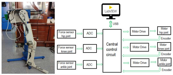
Figure 3. The experiment model (Left—prototype, Right—device connection diagram).

Model parameters are listed in Table 2.

Table 2. Parameters of the prototype.

Parameters	Thigh Link	Leg Link	Foot Platform
m (g)	650	650	152
L (mm)	310	305	190
DC motor parameter	100 W—12VDC	50 W—12VDC	50 W—12VDC
Motor speed after gear	160,000 pulses/rev	920,200 pulses/rev	920,200 pulses/rev
Encoder resolution	400 pulses/rev	400 pulses/rev	400 pulses/rev
Force sensor (loadcell)	10 kg	5 kg	5 kg

The control circuit performs the following tasks: reading data from encoders and force sensors, controlling motors, and communicating with computers. The computer and microcontroller communicate via a serial communication standard, with communication software written in Labview. The collected data are saved for comparison. To ensure the speed of the reading value process, encoder reading is performed using the microcontroller’s external interrupt. The communication software on the computer uses the VISA function on Labview with a variable baud rate.

4.2. Experimental Scenario

The experimental scenarios on the lower-limb rehabilitation robot model consist of three steps:

Step 1: The calibration of initial parameters for the robot: on the interface software, switch to manual control mode, and move the joints to their initial positions, with joint angles of 0 degrees.

Step 2: The execution of training scenarios for the robot: On the interface software, switch to “Training” mode by pressing the corresponding “Training” button for the joint to be trained. Manually move the joints along the training trajectory. The corresponding joint will move according to the manually applied force by the training instructor. Parameters are saved in the database file, including training time, training trajectory, and force measurements at the mechanism during training. These parameters are used as input parameters for the robot during automated operation. The training trajectory for each joint is different depending on that joint’s range of motion. This trajectory is chosen to ensure the safety of the patient’s lower limbs.

Step 3: The robot performs the pre-trained training scenario automatically. On the software, select the “Run” mode for the corresponding joint for the patient’s training. The robot reads data from the database file, follows the trained trajectory, and performs movements accordingly. During operation, parameters such as time, joint angles, and the forces exerted on the robot are recorded in the database file, and these parameters are also used for processing in the robot controllers. During the automated operation of the robot, external forces are applied to assess its performance and the effects of the controllers. In this step, to evaluate the performance of the controllers, while the robot is running automatically, let the robot run without load or assume that there will be external forces acting on the robot. In the case of load, perform several scenarios: the force acts on the stages in one direction with the load being heavy objects weighing 100 g, 200 g, or 500 g; and the force acts in two directions by applying external force with human hands. In addition, change the role of force and motion controllers on the robot with different controller coefficients. The trajectories and force values measured at the joints are recorded and compared with the values measured in step 2.

4.3. Choosing Parameters of the Controllers

We select parameters of the combined controller by trial and error using the experiment setup with position and force controllers, with the following procedures:

(a)

For the position controller: We try different controller parameters and run the systems with different pre-set trajectories, as shown in step 3 above. In each case, we calculate and compare between the pre-set trajectory and measured trajectory. Errors are estimated by using the integral squared error standard ($J_{\mathrm{I}\mathrm{S}\mathrm{E}}$).

We tune the controller’s parameters as follows: (i) we select and fix $K_P$, change $K_D$, and estimate the integral squared error to select $K_D$; (ii) we select and fix $K_D$, change $K_P$, and estimate the integral squared error to select $K_P$.

After several experiments, we received results, as shown in Table 3, with $K_D$ = 2, changing $K_P$ from 0.1 to 0.25. The integral squared error $J_{\mathrm{I}\mathrm{S}\mathrm{E}}$ is shown in Table 3, with the tracking angles shown in Figure 4.

Table 3. Turning position controller’s parameters.

Case	${\mathit{K}}_{\mathit{D}}$	${\mathit{K}}_{\mathit{P}}$	${\mathit{J}}_{\mathbf{I}\mathbf{S}\mathbf{E}}$
Case 1	2	0.1	0.0101
Case 2	2	0.15	0.0051
Case 3	2	0.2	0.0031
Case 4	2	0.25	0.0156

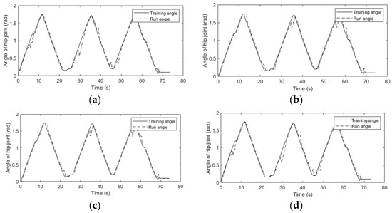
Figure 4. Tracking angles with different controller’s parameters ((a)—case 1, (b)—case 2, (c)—case 3 and (d)—case 4).

When trying $K_P<0.1$ or $K_P>0.25$ and estimated integral squared error $J_{\mathrm{I}\mathrm{S}\mathrm{E}}$, we received bigger errors. The smallest $J_{\mathrm{I}\mathrm{S}\mathrm{E}}$ was received when $K_P$ ranged from 0.15 to 0.2.

(b)

For the force controller: Similar to the position controller, the force controller’s parameters are determined by experiments. With several experiments, for different $w_I$ and $w_D$ values, it can be seen that changing these parameters within a certain range does not show any major influence on the training trajectory or the force acting on the robot. Therefore, we select $w_I=1$ and $w_D=1$. Next, we carry out experiments by changing $w_P$. In each test, change $w_P$ and consider the joint trajectory and the maximum force $F_{max}$ acting on the robot so that the joint can move; then, the appropriate parameters of the controller can be selected. Many experiments with different values of $w_P$ were performed. Table 4 shows the maximum force value $F_{max}$ acting on the robot, so that the joint can move in a number of tests, and Figure 5 depicts the joint trajectories and corresponding moment graphs.

Table 4. Turning force controller’s parameters.

Case	${\mathit{w}}_{\mathit{I}}$	${\mathit{w}}_{\mathit{D}}$	${\mathit{w}}_{\mathit{P}}$	${\mathit{F}}_{\mathit{m}\mathit{a}\mathit{x}}$
Case 1	1	1	0.1	1.27
Case 2	1	1	0.2	1.13
Case 3	1	1	0.5	1.07
Case 4	1	1	0.8	0.75

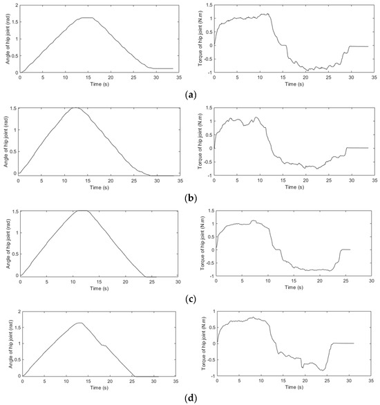Figure 5. Joint trajectories and corresponding forces ((a)—case 1, (b)—case 2, (c)—case 3 and (d)—case 4).

Thus, through conducting experiments by the trial and error method, the controller’s parameters are selected: The parameters of the position controller are $K_D$ = 2 and $K_P$ = 0.15. The parameters of the force controller are $w_I=1,$ $w_D=1 \mathrm{a}\mathrm{n}\mathrm{d} w_p=0.8$. These parameters will be used in experiments with training scenarios with experimental results presented in the next content.

4.4. Results and Discussion

Set 1. Create the reference motion trajectory by performing the training mode: Perform steps 1 and 2 in the experimental scenarios. Collect the joint-angle data measured by encoders to create reference motion trajectories for the robot (see Figure 6a).

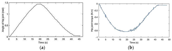
Figure 6. The reference motion trajectory (a) and reference toque of the hip joint (b).

These trajectories are the reference input for the position controller during the automatic training phase conducted in step 3. During operation, experiments at all three joints showed similar results. Among them, the hip joint is heavily loaded, and controlling activities in this joint is the most difficult. If the experimental results at the hip joint meet the requirements, the results achieved at the remaining two joints will also meet expectations. In the following, the experimental results of the system in hip-joint control are presented and analyzed.

Set 2. Create the reference torque: Performing the automatic mode with no external forces and measuring the torque in each joint, we have the reference torque. They will be the torque input of the force controller for experimental cases when the robot runs automatically with external force. As a result, we obtain the reference torque graph, as shown in Figure 6b.

Set 3. Experiment with robot control in cases of external forces: The experiment was carried out in two cases: an external force acts on the joints in one direction, changing the different external force values 1 N, 2 N, and 5 N; external forces of unknown values act on the joints in two directions. External forces are perturbations influencing the system dynamics during the robot’s operational phase. Joint-angle trajectory is measured by encoders, and interaction force is measured by force sensors and converted into torque, as shown in Figure 7 and Figure 8.

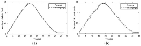
Figure 7. Joint-angle trajectory when an external force acts on the joint in one direction (a); and when an external force of unknown value acts on the joints in two directions (b).

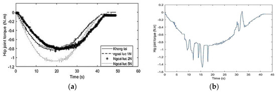
Figure 8. The torque at the hip joint when external forces act in one direction with different external force values (a); and when an external force of unknown value acts in two directions (b).

The experimental results show that in all cases where external forces act on the robot in one or two directions, the position controller always maintains the joint-angle trajectory, following the reference motion trajectory. Using the integral squared error (ISE) standard to evaluate the error between the robot’s motion trajectory and the reference trajectory, we obtain the results shown in Table 5. This result shows that the error between the motion trajectory and the reference trajectory is very small, and the controller has good performance in position control.

Table 5. Trajectory error evaluation.

Cases	Integral Squared Error
No applied force	JISE = 0.0012
The applied force of 1N	JISE1 = 0.0012
The applied force of 2N	JISE2 = 0.0009635
The applied force of 5N	JISE3 = 0.0011

With the force controller, Figure 6 shows the torque value in cases where there is no applied force, as well as applied forces of 1 N, 2 N, and 5 N acting in one direction on the robot. The torque value when no applied force exists is also the reference moment in force control cases when an external force is applied.

This result shows that in all cases, the force controller generated and maintained interaction force. When external forces of different values act on the robot, thanks to the force controller, the torque at the hip joint still has the same value as the reference torque value. However, in the case of larger external force, when the hip joint moves up, the torque output also has a larger value than the reference torque; the maximum error is about 0.3 Nm and still within acceptable values. In case a larger force is applied in both directions, the motion trajectory will also be changed by the external force, but immediately after that, the controller returns the joint angle to the reference trajectory. The ISE value in this case is 0.0020. Although the interaction force at the joint changes significantly when the hip joint moves up, in general, the torque still follows the reference torque value.

We also compare the normal PID controller [17], the compensative gravity PD controller [22], and our proposed combined controller. The experimental results on our system have shown that the proposed controller has a good tracking performance when we applied different forces on the robot.

5. Conclusions

In this paper, a combined position–force control method for a 3 DOF lower-limb rehabilitation robot has been proposed. This control method has been implemented based on the gravity-compensation PD control algorithm and the force feed-forward control algorithm to create a rehabilitation robot that can support patients in performing rehabilitation exercises after a stroke during both passive and active phases. The gravity-compensation PD control algorithm alone can not eliminate disturbances when patients interact with the robot. Therefore, when we combined this controller with force feed-forward control, the controlled trajectory is maintained well, with or without patients. In addition, ways to connect devices to create a robot system capable of communication between therapists, robots, and computers have also been implemented. This allows therapists to easily set exercise parameters and collect and save patient information on the computer to monitor the patient’s exercise and rehabilitation process. The experiment was carried out according to a scenario built on lower-limb rehabilitation exercises for patients after a stroke. The results show that with the proposed controller, the robot operates stably, and flexibly, and supports patients in performing passive and active exercises in different stages of the rehabilitation process.

In the future, research will continue to be carried out with more complete experiments to improve the quality of the controller and robot system, toward the possibility of applying this robot for use in the field of rehabilitation at medical facilities.

References

- Williams, G.R.; Jiang, J.G.; Matchar, D.B.; Samsa, G.P. Incidence and occurrence of total (first-ever and recurrent) stroke. Stroke 1999, 30, 2523–2528. [Google Scholar] [CrossRef] [PubMed]
- Mirelman, A.; Bonato, P.; Deutsch, J.E. Effects of training with a robot-virtual reality system compared with a robot alone on the gait of the individual after stroke. Stroke 2009, 40, 169–174. [Google Scholar] [CrossRef] [PubMed]
- Probosz, K.; Wcislo, R.; Otfinowski, J.; Slota, R.; Kitowski, J.; Pisula, M.; Sobczyk, A. A multime-dia holistic rehabilitation method for patients after stroke. Cyber Psychol. Behav. 2009, 12, 646–647. [Google Scholar]
- Hesse, S.; Schmidt, H.; Werner, C.; Bardeleben, A. Upper and lower extremity robotic rehabilitation devices and for studying motor control. Curr. Opin. Neurol. 2003, 16, 705–710. [Google Scholar] [CrossRef] [PubMed]
- Bradley, D.; Acosta-Marquez, C.; Hawley, M.; Brownsell, S.; Enderby, P.; Mawson, S. Nexos-the design, development, and evaluation of a rehabilitation system for the lower limbs. Mechatronics 2009, 19, 247–257. [Google Scholar] [CrossRef]
- Craig, C.; Jonathan, T.; Stephen, R. Development of an exoskeleton haptic interface for virtual task training. In Proceedings of the 2009 IEEE/RSJ International Conference on Intelligent Robots and Systems, St. Louis, MO, USA, 10–15 October 2009; pp. 3697–3702. [Google Scholar]
- Langhorne, P.; Coupar, F.; Pollock, A. Motor recovery after stroke: A systematic review. Lancet Neurol. 2009, 8, 741–754. [Google Scholar] [CrossRef]
- Mayr, A.; Kofler, M.; Quirbach, E.; Matzak, H.; Frohlich, K.; Saltuari, L. Prospective, blinded, randomized cross-over study of gait rehabilitation in stroke patients using the Lokomat gait orthosis. Neurorehabilit. Neural Repair 2007, 21, 307–314. [Google Scholar] [CrossRef]
- Thielman, G.T.; Dean, C.M.; Gentile, A.M. Rehabilitation of reaching after stroke: Task-related training versus progressive resistive exercise. Arch. Phys. Med. Rehabil. 2004, 85, 1613–1618. [Google Scholar] [CrossRef]
- Riener, R.; Lunenburger, L.; Jezernik, S.; Anderschitz, M.; Colombo, G.; Dietz, V. Patient-cooperative strategies for robot-aided treadmill training: First experimental results. IEEE Trans. Neural Syst. Rehabil. Eng. 2005, 13, 380–394. [Google Scholar] [CrossRef]
- Veneman, J.F.; Kruidhof, R.; Hekman EE, G.; Ekkelenkamp, R.; Van Asseldonk, E.H.F.; vander Kooij, H. Design and evaluation of the Lopes exoskeleton robot for interactive gait rehabilitation. IEEE Trans. Neural Syst. Rehabil. Eng. 2007, 15, 379–386. [Google Scholar] [CrossRef]
- Freivogel, S.; Mehrholz, J.; Husak-Sotomayor, T.; Schmalohr, D. Gait training with the newly developed ‘LokoHelp’-System is feasible for non-ambulatory patients after stroke, spinal cord, and brain injury. A feasibility study. Brain Inj. 2008, 22, 625–632. [Google Scholar] [CrossRef] [PubMed]
- Meuleman, J.; van Asseldonk, E.; van Oort, G.; Rietman, H.; van der Kooij, H. LOPES II—Design and evaluation of an admittance-controlled gait training robot with a shadow leg approach. IEEE Trans. Neural Syst. Rehabil. Eng. 2016, 24, 352–363. [Google Scholar] [CrossRef] [PubMed]
- Do, T.; Vu, D.T. A Simple Control Method for Exoskeleton for Rehabilitation. SSRG Int. J. Electr. Electron. Eng. (SSRG-IJEEE) 2017, 4, 7–12. [Google Scholar] [CrossRef]
- Ranaweera, R.K.P.S.; Jayasiri, W.A.T.I.; Tharaka, W.G.D.; Gunasiri, J.H.H.P.; Gopura, R.A.R.C.; Jayawardena, T.S.S.; Mann, G.K.I. Anthro-X: Anthropomorphic Lower Extremity Exoskeleton Robot for Power Assistance. In Proceedings of the 2018 4th International Conference on Control, Automation and Robotics (ICCAR), Auckland, New Zealand, 20–23 April 2018; pp. 82–87. [Google Scholar]
- Moreno, J.C.; Figueiredo, J.; Pons, J.L. Chapter 7 exoskeletons for lower-limb rehabilitation. In Rehabilitation Robotics; Colombo, R., Sanguineti, V., Eds.; Academic Press: New York, NY, USA, 2018; pp. 89–99. [Google Scholar]
- Herianto, H.; Saryanto, W.Y.; Cahyadi, A.I. Modeling and Design of Low-Cost Lower Limb Rehabilitation Robot Control System for Post-Stroke Patient using PWM Controller. Int. J. Mech. Mechatron. Eng. IJMME-IJENS 2016 2016, 16, 101–108. [Google Scholar]
- Mergner, T.; Lippi, V. Posture control-human-inspired approaches for humanoid robot benchmarking: Conceptualizing tests, protocols, and analysis. Front. Neurorobotics 2018, 12, 21. [Google Scholar] [CrossRef]
- Deng, M.Y.; Ma, Z.Y.; Wang, Y.N.; Wang, H.S.; Zhao, Y.B.; Wei, Q.X.; Yang, W.; Yang, C.J. Fall preventive gait trajectory planning of a lower limb rehabilitation exoskeleton based on capture point theory. Front. Inf. Technol. Electr. Eng. 2019, 20, 1322–1330. [Google Scholar] [CrossRef]
- Thang, N.C.; Manukid, P.; Tra My, P.T.; Gam LT, H.; Chung, P.N.; Hieu, N.N. Force Control of an Upper limb Exoskeleton for Perceiving Reality using Force Feed Forward Model. In Proceedings of the 5th International Conference on Engineering Mechanics and Automation (ICEMA 5), Hanoi, Vietnam, 11–12 October 2019; pp. 331–337. [Google Scholar]
- Sun, W.; Lin, J.-W.; Su, S.-F.; Wang, N.; Er, M.J. Reduced adaptive fuzzy decoupling control for lower limb exoskeleton. IEEE Trans. Cybern. 2020, 51, 1099–1109. [Google Scholar] [CrossRef]
- Gam, L.T.H.; Quan, D.H.; Thanh, B.T.; Van Bach Ngoc, P. Advanced Method for Motion Control of a 3 DOF Lower Limb Rehabilitation Robot. Int. J. Innov. Technol. Interdiscip. Sci. 2019, 2, 316–325. [Google Scholar]
- Slade, P.; Kochenderfer, M.J.; Delp, S.L.; Collins, S.H. Personalizing exoskeleton assistance while walking in the real world. Nature 2022, 610, 277–282. [Google Scholar] [CrossRef]
- Luo, S.; Androwis, G.; Adamovich, S.; Nunez, E.; Su, H.; Zhou, X. Robust walking control of a lower limb rehabilitation exoskeleton coupled with a musculoskeletal model via deep reinforcement learning. J. NeuroEngineering Rehabil. 2023, 20, 34. [Google Scholar] [CrossRef]
- Frisoli, A.; Borelli, L.; Montagner, A.; Marcheschi, S.; Procopio, C.; Salsedo, F.; Bergamasco, M.; Carboncini, M.C.; Tolaini, M.; Rossi, B. Arm rehabilitation with a robotic exoskeleton in virtual reality. In Proceedings of the 2007 IEEE 10th International Conference on Rehabilitation Robotics, Noordwijk, The Netherlands, 13–15 June 2007; pp. 631–642. [Google Scholar]
- Vertechy, R.; Frisoli, A.; Dettori, A.; Solazzi, M.; Bergamasco, M. Development of a new exoskeleton for upper limb rehabilitation. In Proceedings of the 2009 IEEE International Conference on Rehabilitation Robotics, Kyoto, Japan, 23–26 June 2009; pp. 188–193. [Google Scholar]
- Şahin, Y.; Botsalı, F.M.; Kalyoncu, M.; Tinkir, M.; Önen, Ü.; Yılmaz, N.; Baykan, Ö.K.; Çakan, A. Force Feedback Control of Lower Extremity Exoskeleton Assisting of Load Carrying Human. Appl. Mech. Mater. 2014, 598, 546–550. [Google Scholar] [CrossRef]
- Perry, J.C.; Rosen, J.; Burns, S. Upper arm power exoskeleton design. IEEE/ASME Trans. Mechatron. 2007, 12, 408–417. [Google Scholar] [CrossRef]
- Chen, G.; Qi, P.; Guo, Z.; Yu, H. Mechanical design and evaluation of a compact portable knee–ankle–foot robot for gait rehabilitation. Mech. Mach. Theory 2016, 103, 51–64. [Google Scholar] [CrossRef]
- Tsai, L.-W. Robot Analysis—The Mechanics of Serial and Parallel Manipulators; A Wiley-Interscience Publication: Hoboken, NJ, USA, 1999. [Google Scholar]
- Jamwal, P.K.; Xie, S.Q.; Hussain, S.; Parsons, J.G. An Adaptive Wearable Parallel Robot for the Treatment of Ankle Injuries. IEEE/ASME Trans. Mechatron. 2014, 19, 64–75. [Google Scholar] [CrossRef]
- Lu, R.; Li, Z.; Su, C.Y.; Xue, A. Development and learning control of a human limb with a rehabilitation exoskeleton. IEEE Trans. Ind. Electron. 2014, 61, 3776–3785. [Google Scholar] [CrossRef]
- Martin, P.; Emami, M.R. Aneuro-fuzzy approach to real-time trajectory generation for robotic rehabilitation. Robot. Auton. Syst. 2014, 62, 568–578. [Google Scholar] [CrossRef]
- Ju, M.S.; Lin, C.C.K.; Lin, D.H.; Hwang, I.S.; Chen, S.M. A rehabilitation robot with force-position hybrid fuzzy controller: Hybrid fuzzy control of rehabilitation robot. IEEE Trans. Neural Syst. Rehab Eng. 2005, 13, 349–358. [Google Scholar]
Disclaimer/Publisher’s Note: The statements, opinions and data contained in all publications are solely those of the individual author(s) and contributor(s) and not of MDPI and/or the editor(s). MDPI and/or the editor(s) disclaim responsibility for any injury to people or property resulting from any ideas, methods, instructions or products referred to in the content. |
© 2024 by the authors. Licensee MDPI, Basel, Switzerland. This article is an open access article distributed under the terms and conditions of the Creative Commons Attribution (CC BY) license (https://creativecommons.org/licenses/by/4.0/).