Overbounding the Model Uncertainty for Kalman Filter-Based Advanced Receiver Autonomous Integrity Monitoring in the Presence of Time Correlation by the Hybrid Evolutionary Algorithm

Abstract

Overbounding the integrity risk is a significant challenge for Kalman filter (KF)-based advanced receiver autonomous integrity monitoring (ARAIM) when the measurement error has an uncertain time correlation. Thus, this paper presents a method that addresses this challenge by effectively bounding the integrity risk for KF-based ARAIM while considering the uncertainty in the model of the time-correlated error. Firstly, the recursive equation for covariance is derived, establishing a direct mathematical expression that links the integrity risk and the correlation time constant. Subsequently, a min–max optimization model is constructed, utilizing the obtained expression as the objective function, to simultaneously bound the integrity risk and reduce conservatism. To effectively address the current min–max optimization problem, a hybrid evolutionary algorithm is proposed, which conducts global searching followed by local searching. The simulation result demonstrates that it outperforms other algorithms, enabling rapid attainment of the minimum upper bound on the integrity risk.

1. Introduction

With the availability of multiple constellations and dual frequencies, advanced receiver autonomous integrity monitoring (ARAIM) has been developed to support stringent services with vertical guidance, e.g., a localizer precision vertical 200 feet decision height (LPV-200) [1,2]. Several required navigation performance indicators have been defined to evaluate the navigation systems in civil aviation applications by the International Civil Aviation Organization (ICAO) [3]. Among these indicators, integrity is a measure of the trust that can be placed in the correctness of the information supplied by the total navigation system. The bounding of the integrity risk is essential for assuring the safety of aircraft operation, which is quantitatively expressed by the probability of hazardously misleading information [4].

By using carrier-smoothed code measurements from multiple satellites at a single epoch, the snapshot algorithm is used in the existing ARAIM implementation [2]. In recent years, some studies have focused on the time-sequential algorithm to accurately quantify the integrity risk for ARAIM [4,5,6]. Among these sequential implementations, the Kalman filter (KF)-based algorithm is a representative estimator that exploits using the information from both the measurements and the system’s dynamic model. The KF is a powerful estimation algorithm [7], which has been widely used in many areas such as in autonomous vehicles [8], economic applications [9], and computer versions [10]. Normally, the traditional KF is used in the linear system, while for the nonlinear filtering problem, several extensions have been proposed such as the extended Kalman filter (EKF) and unscented Kalman filter (UKF) [11].

Compared with the snapshot algorithm relying on a single measurement alone, the KF-based algorithm can utilize sequential measurements to recursively obtain optimal current-time state estimates, which maximizes current-time accuracy and integrity performance [12]. Typically, satellite measurement errors are assumed to be Gaussian white noises when using a KF [13]. However, this is improper for applications where the existence of time-correlated errors degrades the KF accuracy and reliability of integrity risk evaluation [14]. Therefore, one major challenge with KF estimation in ARAIM is determining how to account for time-correlated errors such as the multipath error. Approaches based on measurement differencing between adjacent epochs are conventionally applied to decouple the time-correlated component from the measurement error in KF [15,16,17]. However, some practical drawbacks, i.e., time latency and numerical issues from matrix inversion, limit their use. Generally, the time-correlated error can be modeled well as the Gauss–Markov process (GMP) [18]. Then, the state augmentation technique [19] can be used to incorporate time-correlated errors in the original state vector, thus whitening the measurement noise in a KF. However, precise time constant values in the GMP are still difficult to obtain because of the uncertainty in the true nature of the time correlation. As illustrated in this study, if the model in the filter cannot represent the actual time-correlated error exactly, there is uncertainty in the standard a posteriori covariance matrix, which may result in a loss of integrity.

The bounding of the integrity risk in the presence of uncertain time correlation has been studied extensively. Based on the upper and lower bounds of the autocorrelation function (ACF), the upper bound of the estimated error variance was derived for sequential state estimators [20,21,22]. To solve the limitation of lower-bounding the negative value of an empirical ACF, Ref. [23] used the products of samples taken at different times to bound the sample cumulative distribution function, thereby providing bounds on the sample time correlation. Further, Ref. [24] exploited the Fourier transform of an ACF, i.e., power spectral density (PSD), to overbound KF-based estimated error distribution. Furthermore, this frequency-domain method was used to derive tight upper bounds for the estimated error variance with the assumption that the actual error was modeled as a first-order GMP with uncertainty for the time constant and the variance [18]. Furthermore, an upper bound on the estimated error variance in KF was derived by establishing the positive semi-definiteness of the difference between the true covariance matrix and the constructed matrix when the time constant of the first-order GMP lay within a specified interval [25,26,27]. By constructing the estimated error covariance with the true time constant and the parameter specified by the filter designer, the minimum upper bound on the estimated error variance is defined as a min–max optimization problem, whose solution is solved by a brute-force search for all values of the time constant in the range [28].

However, the relevant research is still lacking for the bounding of the integrity risk in the presence of an uncertain time correlation in KF-based ARAIM, and the existing methods mentioned above are inapplicable due to two limitations. The first limitation is the completely different definition of the integrity risk. In the above references, the integrity risk is defined as the probability that the estimated error exceeds a specified number; that is, the bounding of the integrity risk can be achieved by solely obtaining the upper bound of the estimated error variance in KF. However, this is not the case in ARAIM where the integrity risk is defined as the probability that the estimated error exceeds the alert limit and the detection test statistics smaller than the threshold simultaneously. Specifically, two other variances, i.e., the subset estimated error variance and the variance in the difference between the all-in-view solution and the subset solution, are needed to be considered in the evaluation of the integrity risk in ARAIM, besides the estimated error variance. More importantly, the relationship between the integrity risk and the variances is nonlinear, whereas it is defined as a linear one in the previous references. Thus, given that the uncertainty in the correlation time constant impacts these three variances simultaneously, it would be wise to establish a direct mathematical expression to link the integrity risk and the correlation time constant rather than simply proposing the method to obtain an upper bound for the variance. To guarantee the bounding of the integrity risk and reduce conservatism at the same time, the min–max model is then built adopting the predefined mathematical expression as the objective function.

The second limitation is the efficiency when solving the min–max optimization problem. As mentioned above, brute-force searching is used in [28], which is impractical and computationally extensive. In the last decade, an abundance of works have been studied to solve the min–max optimization problem using the numerical method, which has been applied in many areas such as game theory [29], signal processing [30], and machine learning [31]. These numerical methods can be categorized into two types. One is gradient-based algorithms such as the gradient descent–ascent algorithm [32,33], which utilizes the gradient descent and ascent to determine the direction in the minimization and maximization search spaces, respectively. However, gradient-based algorithms cannot be applied to the current problem, which is limited by the following two fronts. First, it is difficult to obtain the analytic expression for derivatives of the objective function in this work. Second, the gradient-based algorithm is heavily dependent on the initial approximation of solution and easily falls into local optimal solution. In other words, the derivation relies on the assumption of continuity, and local optimization requires the condition of convexity. However, the min–max optimization in this work is a global optimal problem, and the objective function is non-convex and non-concave. Within a specified interval of the variable, it is almost impossible to select an initial value that is just within the local range of the global optimal solution.

The other type is the evolutionary algorithm (EA), which is a heuristic-based approach simulating natural evolution and social behaviors. Compared with gradient-based algorithms, EAs do not make any assumptions regarding continuity and convexity on the objective function and only requires the value of the objective function without the derivative information [34]. So, several EAs have been proposed to solve the min–max problem, such as the co-evolutionary genetic algorithm (GA) [35,36], co-evolutionary particle swarm optimization (PSO) [37,38], and the differential evolution algorithm [39]. In these algorithms, two populations focus on evolving the minimization and maximization, respectively, and they interact with each other through the common objective function. Unfortunately, the results from these algorithms are not stable when setting small values of population size and the number of generations, indicating the integrity risk is not guaranteed to be bounded. On the other hand, a large amount of time is consumed when large values are set to the population size and the number of generations.

Since the bounding of integrity risk directly relates to the safety of the airplane, it is essential to solve this problem for KF-based ARAIM. Thus, this paper identifies this critical problem and proposes a method for overbounding the integrity risk for KF-based ARAIM given that the uncertainty in the model of time-correlated error is considered. First, inspired by the idea set forth in [28] and the propagation of states in the discrete-time system [19], this paper provides a new derivation of two variances, i.e., the variance in the difference between the all-in-view solution and the subset solution and the subset estimated error, which is used to establish a direct mathematical expression to link the integrity risk and the correlation time constant. Then, to bound the integrity risk and reduce conservatism simultaneously, a min–max model is built where the objective function is the predefined mathematical expression. In contrast to the one in Reference [28], the current min–max model introduces a more complex objective function, which makes it much more challenging to solve the optimization problem. Finally, the proposed hybrid evolutionary algorithm is specialized to address the above min–max problem. In inner and outer problems, the proposed algorithm firstly determines the global optimal area and then rapidly finds the optimal solution in this local area.

This paper is organized as follows. First, the time-correlated error model in the integrity risk evaluation for KF-based ARAIM is described, and the existing problem is stated in detail. Second, the recursive covariance matrices are derived to bound the effect of uncertain parameters on variances. Third, a min–max mathematical model is built to bound the integrity risk and reduce conservatism simultaneously for KF-based ARAIM. Fourth, a hybrid evolutionary algorithm is proposed to solve the min–max optimization problem. Finally, a conclusion is given.

2. Problem Statement

Normally, a linear dynamic system can be described by the measurement and process equations in KF where measurement errors are assumed to be white Gaussian noises. However, the time-correlated error exists in the measurement, such as the multipath, which is generally modeled as a first-order GMP [4]. Thus, the state augmentation technique [19] incorporates time-correlated errors in the original state vector to whiten the measurement noise as follows:

$$\begin{array}{c}{\mathit{z}}_k=[{\mathit{H}}_k^{*}\mathit{I}]\left[\begin{array}{c}{\mathit{x}}_k^{*}\\ {\mathit{m}}_k\end{array}\right]+{\mathit{n}}_k+{\mathit{f}}_k\\ \left[\begin{array}{c}{\mathit{x}}_{k+1}^{*}\\ {\mathit{m}}_{k+1}\end{array}\right]=\left[\begin{array}{cc}{\mathit{\Phi }}_k& \mathbf{0}\\ \mathbf{0}& e^{-{\displaystyle \frac{\Delta t}{\tau }}}\mathit{I}\end{array}\right]\left[\begin{array}{c}{\mathit{x}}_k^{*}\\ {\mathit{m}}_k\end{array}\right]+\left[\begin{array}{c}{\mathit{w}}_k\\ {\mathit{\eta }}_k\end{array}\right]\end{array}$$

(1)

where ${\mathit{z}}_k$ is the $q_k\times 1$ measurement vector, ${\mathit{H}}_k^{*}$ is the $q_k\times p_k$ observation matrix, $\mathit{I}$ is an identity matrix, and ${\mathit{x}}_k^{*}$ is the $p_k\times 1$ original state vector. ${\mathit{f}}_k$ is the $q_k\times 1$ fault vector, where if the corresponding measurement of the element comes from a faulty satellite, then the element is one. The subscript $k$ indicates any discrete time of a time sequence. The zero-mean white Gaussian noise vector ${\mathit{n}}_k$ is $q_k\times 1$ with the covariance matrix ${\mathit{N}}_k$. The time-correlated error vector ${\mathit{m}}_k$ is $q_k\times 1$, where the element is modeled as a discrete sequence of the first-order GMP specified by a time constant $\tau$ and a variance ${\sigma }^2$ [27]. $\Delta t$ is the sampling interval, and $q_k\times 1$ vector ${\mathit{\eta }}_k$ is a white noise sequence with the covariance matrix ${\sigma }^2(1-e^{-{\displaystyle \frac{2\Delta t}{\tau }}})\mathit{I}$. ${\mathit{\Phi }}_k$ is the $p_k\times p_k$ state transition matrix, and ${\mathit{w}}_k$ is the $p_k\times 1$ process noise vector.

With ${\mathit{x}}_k=\left[\begin{array}{c}{\mathit{x}}_k^{*}\\ {\mathit{m}}_k\end{array}\right]$, Equation (1) is simplified as follows:

$$\begin{gathered} {\mathit{z}}_k={\mathit{H}}_k{\mathit{x}}_k+{\mathit{n}}_k+{\mathit{f}}_k \\ {\mathit{x}}_{k+1}={\mathit{F}}_k{\mathit{x}}_k+{\mathit{S}}_k \end{gathered}$$

(2)

where the definitions of ${\mathit{H}}_k$, ${\mathit{F}}_k$, and ${\mathit{s}}_k$ are obvious from comparing Equations (1) and (2).

As for the integrity risk, or probability of hazardously misleading information $P_{HMI}$, in ARAIM, it is defined as the probability that the estimated error exceeds the alert limit, and the detection test statistic is smaller than the threshold at the same time [4,12]:

$$P_{HMI}\le P\left(|{\epsilon }_0|>l|H_0\right)P_{H_0}+{{\displaystyle \sum }}_{i=1}^{h}P(|{\epsilon }_i|+T_{{\Delta }_i}>l|H_i)P_{H_i},$$

(3)

where ${\epsilon }_0$ and ${\epsilon }_i$ are the estimated errors of the parameter of interest using all-in-view satellites and subset $i$, respectively. $l$ is the specified alert limit that defines the hazardous situation, $H_0$ is the fault-free hypothesis, and $H_i$ for $i=1\cdots h$ is a set of fault hypotheses corresponding to faults for subset $i$. $P_{H_0}$ and $P_{H_i}$ are the prior probabilities of $H_0$ and $H_i$ occurrences, respectively, and $T_{{\Delta }_i}$ is the detection threshold for subset $i$.

For each subset, the calculation of $T_{{\Delta }_i}$ is based on an allocated continuity budget [4]:

$$T_{{\Delta }_i}=Q^{-1}\left(x\right)=Q^{-1}({\displaystyle \frac{C_{REQ}}{2P_{H_0}h}}){\sigma }_{{\Delta }_i},$$

(4)

where $Q^{-1}\left(x\right)$ is the inverse tail probability function of $x$, $C_{REQ}$ is the allocated continuity risk requirement to limit the probability of false alarms, and ${\sigma }_{{\Delta }_i}$ is the standard deviation of the difference between the all-in-view solution and the subset solution.

By substituting Equation (4) into Equation (3), the $P_{HMI}$ bound can be expressed as follows:

$$P_{HMI}\le 2Q\left({\displaystyle \frac{l}{{\sigma }_0}}\right)P_{H_0}+{{\displaystyle \sum }}_{i=1}^{h}2Q\left({\displaystyle \frac{l-Q^{-1}\left(\frac{C_{REQ}}{2P_{H_0}h}\right){\sigma }_{{\Delta }_i}}{{\sigma }_{{\epsilon }_i}}}\right)P_{H_i},$$

(5)

where $Q\left(x\right)$ is the tail probability function of $x$. ${\sigma }_0$ and ${\sigma }_{{\epsilon }_i}$ are standard deviations of the all-in-view and subset estimated errors, respectively.

Since it is difficult to accurately measure the correlation time constant $\tau$, only a rough value can be obtained with post-processing data [40], which can cause uncertainty in the evaluation of the integrity risk. As mentioned before, the proposed methods in the references are only used to bound the integrity risk by obtaining the upper bound of ${\sigma }_0$. In Equation (5), it is evident that simply obtaining an upper bound of ${\sigma }_0$ is insufficient to bound $P_{HMI}$ in ARAIM. Given that the uncertainty in the correlation time constant impacts ${\sigma }_0$, ${\sigma }_{{\epsilon }_i}$, and ${\sigma }_{{\Delta }_i}$ simultaneously, it would be wise to establish a direct mathematical expression that connects the integrity risk and the correlation time constant instead of solely proposing the method to obtain an upper bound for the variance. To establish such mathematical expression, the following section is used to derive the recursive equation for the above variances.

3. Derivation of Modified Covariance

This section provides a new derivation of the recursive equation for ${\sigma }_{{\Delta }_i}$ and ${\sigma }_{{\epsilon }_i}$, which is used to establish the mathematical expression. Compared with the derivation of the standard deviation for the estimated error in Reference [28], the derivation of ${\sigma }_{{\Delta }_i}$ and ${\sigma }_{{\epsilon }_i}$ is notably more intricate, particularly for ${\sigma }_{{\Delta }_i}$. This complexity arises from several factors. First, ${\sigma }_{{\Delta }_i}$ represents the standard deviation of the difference between the all-in-view solution and the subset solution, which cannot be directly obtained using the standard KF equations. Consequently, the recursive covariance matrix required to calculate ${\sigma }_{{\Delta }_i}$ encompasses nine matrix elements, which is considerably larger than the number in the reference, significantly augmenting the computational complexity involved in the calculation. Second, the subset error necessitates the introduction of a coefficient matrix to extract fault-free measurements, which further adds to the complexity of the calculation. Furthermore, we enhance computational efficiency by integrating the recursive covariance matrices of ${\sigma }_{{\Delta }_i}$ and ${\sigma }_{{\epsilon }_i}$ into a single recursive covariance matrix. Additionally, when determining the initial covariance matrix, expectations for nine matrix elements are derived, as opposed to four in the reference, which again amplifies the complexity of the process.

In what follows, the detailed derivation is described. Based on Equation (2), obtaining the a priori estimated error ${\overline{\mathit{\epsilon }}}_k$ is straightforward:

$$\begin{array}{cc}{\overline{\mathit{\epsilon }}}_k\hfill & ={\mathit{x}}_k-{\overline{\mathit{x}}}_k\hfill \\ & ={\mathit{F}}_{k-1}{\mathit{x}}_{k-1}+{\mathit{s}}_{k-1}-{\tilde{\mathit{F}}}_{k-1}{\widehat{\mathit{x}}}_{k-1}\hfill \\ & ={\tilde{\mathit{F}}}_{k-1}\left({\mathit{x}}_{k-1}-{\widehat{\mathit{x}}}_{k-1}\right)+\left({\mathit{F}}_{k-1}-{\tilde{\mathit{F}}}_{k-1}\right){\mathit{x}}_{k-1}+{\mathit{s}}_{k-1}\hfill \\ & ={\tilde{\mathit{F}}}_{k-1}{\widehat{\mathit{\epsilon }}}_{k-1}+\Delta {\mathit{F}}_{k-1}{\mathit{x}}_{k-1}+{\mathit{s}}_{k-1}\hfill \end{array},$$

(6)

where “${\overline{\mathit{x}}}_k$” denotes the estimate at time $k$ given the observations up to and including times $k-1$, while “${\widehat{\mathit{x}}}_k$” denotes the estimate at time $k$ given the observations up to and including times $k$. ${\tilde{\mathit{F}}}_{k-1}$ denotes that the uncertain parameter is used in the dynamic model.

The KF a posteriori estimated state is ${\widehat{\mathit{x}}}_k={\mathit{K}}_k{\mathit{z}}_k+\left(\mathit{I}-{\mathit{K}}_k{\mathit{H}}_k\right){\overline{\mathit{x}}}_k$, and the a posteriori estimated error ${\widehat{\mathit{\epsilon }}}_k$ is defined as follows:

$$\begin{array}{cc}{\widehat{\mathit{\epsilon }}}_k\hfill & ={\mathit{x}}_k-{\widehat{\mathit{x}}}_k\hfill \\ & ={\mathit{x}}_k-{\mathit{K}}_k{\mathit{z}}_k-\left(\mathit{I}-{\mathit{K}}_k{\mathit{H}}_k\right){\overline{\mathit{x}}}_k\hfill \\ & ={\mathit{x}}_k-{\mathit{K}}_k\left({\mathit{H}}_k{\mathit{x}}_k+{\mathit{n}}_k+{\mathit{f}}_k\right)-\left(\mathit{I}-{\mathit{K}}_k{\mathit{H}}_k\right){\overline{\mathit{x}}}_k\hfill \\ & =\left(\mathit{I}-{\mathit{K}}_k{\mathit{H}}_k\right)({\mathit{x}}_k-{\overline{\mathit{x}}}_k)-{\mathit{K}}_k{\mathit{n}}_k-{\mathit{K}}_k{\mathit{f}}_k\hfill \\ & =\left(\mathit{I}-{\mathit{K}}_k{\mathit{H}}_k\right){\overline{\mathit{\epsilon }}}_k-{\mathit{K}}_k{\mathit{n}}_k-{\mathit{K}}_k{\mathit{f}}_k\hfill \end{array},$$

(7)

where ${\mathit{K}}_k$ is the Kalman gain using the model ${\tilde{\mathit{F}}}_{k-1}$.

A similar procedure can be followed to derive the a priori and a posteriori estimated errors, i.e., ${\overline{\mathit{\epsilon }}}_{k,i}$ and ${\widehat{\mathit{\epsilon }}}_{k,i}$ for subset $i$:

$$\begin{array}{cc}{\overline{\mathit{\epsilon }}}_{k,i}\hfill & ={\mathit{x}}_k-{\overline{\mathit{x}}}_{k,i}={\tilde{\mathit{F}}}_{k-1}{\widehat{\mathit{\epsilon }}}_{k-1,i}+\Delta {\mathit{F}}_{k-1}{\mathit{x}}_{k-1}+{\mathit{s}}_{k-1}\hfill \\ \\ {\widehat{\mathit{\epsilon }}}_{k,i}\hfill & ={\mathit{x}}_k-{\widehat{\mathit{x}}}_{k,i}\hfill \\ & =\left(\mathit{I}-{\mathit{K}}_{k,i}{\mathit{B}}_i^T{\mathit{H}}_k\right){\overline{\mathit{\epsilon }}}_{k,i}-{\mathit{K}}_{k,i}{\mathit{B}}_i^T{\mathit{n}}_k-{\mathit{K}}_{k,i}{\mathit{B}}_i^T{\mathit{f}}_k\hfill \end{array},$$

(8)

where ${\mathit{B}}_i={\left[\begin{array}{cc}{\mathbf{0}}_{(q_k-u_i)\times u_i}& {\mathit{I}}_{q_k-u_i}\end{array}\right]}^T$ is used to extract fault-free measurements. $u_i$ is the number of faulted satellites, and it is assumed that faulty measurements are the first $u_i$ elements of ${\mathit{z}}_k$ under fault hypothesis $H_i$.

The a priori and a posteriori differences between the all-in-view position solution and the subset solution, i.e., ${\overline{\Delta }}_{k,i}$ and ${\widehat{\Delta }}_{k,i}$, are calculated by subtracting Equations (6) and (7) from (8):

$$\begin{array}{cc}{\overline{\Delta }}_{k,i}\hfill & ={\overline{\mathit{x}}}_k-{\overline{\mathit{x}}}_{k,i}={\overline{\mathit{\epsilon }}}_{k,i}-{\overline{\mathit{\epsilon }}}_k\hfill \\ & ={\tilde{\mathit{F}}}_{k-1}{\widehat{\mathit{\epsilon }}}_{k-1,i}+\Delta {\mathit{F}}_{k-1}{\mathit{x}}_{k-1}\hfill \\ & \hspace{1em}+{\mathit{s}}_{k-1}-\left({\tilde{\mathit{F}}}_{k-1}{\widehat{\mathit{\epsilon }}}_{k-1}+\Delta {\mathit{F}}_{k-1}{\mathit{x}}_{k-1}+{\mathit{s}}_{k-1}\right)\hfill \\ & ={\tilde{\mathit{F}}}_{k-1}{\widehat{\Delta }}_{k-1,i}\hfill \\ \\ {\widehat{\Delta }}_{k,i}\hfill & ={\widehat{\mathit{x}}}_k-{\widehat{\mathit{x}}}_{k,i}={\widehat{\mathit{\epsilon }}}_{k,i}-{\widehat{\mathit{\epsilon }}}_k\hfill \\ & =\left(\mathit{I}-{\mathit{K}}_{k,i}{\mathit{B}}_i^T{\mathit{H}}_k\right){\overline{\mathit{\epsilon }}}_{k,i}-{\mathit{K}}_{k,i}{\mathit{B}}_i^T{\mathit{n}}_k-{\mathit{K}}_{k,i}{{\mathit{B}}_i^T\mathit{f}}_k\hfill \\ & \hspace{1em}-\left(\left(\mathit{I}-{\mathit{K}}_k{\mathit{H}}_k\right){\overline{\mathit{\epsilon }}}_k-{\mathit{K}}_k{\mathit{n}}_k-{\mathit{K}}_k{\mathit{f}}_k\right)\hfill \\ & =\left(\mathit{I}-{\mathit{K}}_k{\mathit{H}}_k\right){\overline{\Delta }}_{k,i}+\left({\mathit{K}}_k{\mathit{H}}_k-{\mathit{K}}_{k,i}{\mathit{B}}_i^T{\mathit{H}}_k\right){\overline{\mathit{\epsilon }}}_{k,i}\hfill \\ & \hspace{1em}+\left({\mathit{K}}_k-{\mathit{K}}_{k,i}{\mathit{B}}_i^T\right){\mathit{n}}_k+\left({\mathit{K}}_k-{\mathit{K}}_{k,i}{\mathit{B}}_i^T\right){\mathit{f}}_k\hfill \end{array}.$$

(9)

To calculate ${\sigma }_{{\epsilon }_i}$ and ${\sigma }_{{\Delta }_i}$ at the same time to improve efficiency, Equations (2), (8) and (9) are written in a more compact form:

$$\begin{array}{cc}\left[\begin{array}{c}{\overline{\Delta }}_{k,i}\\ {\overline{\mathit{\epsilon }}}_{k,i}\\ {\mathit{x}}_k\end{array}\right]=\hfill & \left[\begin{array}{ccc}{\tilde{\mathit{F}}}_{k-1}& \mathbf{0}& \mathbf{0}\\ \mathbf{0}& {\tilde{\mathit{F}}}_{k-1}& \Delta {\mathit{F}}_{k-1}\\ \mathbf{0}& \mathbf{0}& {\mathit{F}}_{k-1}\end{array}\right]\left[\begin{array}{c}{\widehat{\Delta }}_{k-1,i}\\ {\widehat{\mathit{\epsilon }}}_{k-1,i}\\ {\mathit{x}}_{k-1}\end{array}\right]+\left[\begin{array}{c}\mathbf{0}\\ \mathit{I}\\ \mathit{I}\end{array}\right]{\mathit{s}}_{k-1}\hfill \\ \\ \left[\begin{array}{c}{\widehat{\Delta }}_{k,i}\\ {\widehat{\mathit{\epsilon }}}_{k,i}\\ {\mathit{x}}_k\end{array}\right]=\hfill & \left[\begin{array}{ccc}\left(\mathit{I}-{\mathit{K}}_k{\mathit{H}}_k\right)& \left({\mathit{K}}_k{\mathit{H}}_k-{\mathit{K}}_{k,i}{\mathit{B}}_i^T{\mathit{H}}_k\right)& \mathbf{0}\\ \mathbf{0}& (\mathit{I}-{\mathit{K}}_{k,i}{\mathit{B}}_i^T{\mathit{H}}_k)& \mathbf{0}\\ \mathbf{0}& \mathbf{0}& \mathit{I}\end{array}\right]\left[\begin{array}{c}{\overline{\Delta }}_{k,i}\\ {\overline{\mathit{\epsilon }}}_{k,i}\\ {\mathit{x}}_k\end{array}\right]\hfill \\ & +\left[\begin{array}{c}\left({\mathit{K}}_k-{\mathit{K}}_{k,i}{\mathit{B}}_i^T\right)\\ -{\mathit{K}}_{k,i}{\mathit{B}}_i^T\\ \mathbf{0}\end{array}\right]{\mathit{n}}_k+\left[\begin{array}{c}\left({\mathit{K}}_k-{\mathit{K}}_{k,i}{\mathit{B}}_i^T\right)\\ -{\mathit{K}}_{k,i}{\mathit{B}}_i^T\\ \mathbf{0}\end{array}\right]{\mathit{f}}_k\hfill \end{array}.$$

(10)

These two standard deviations, ${\sigma }_{{\epsilon }_i}$ and ${\sigma }_{{\Delta }_i}$, are the square roots of the corresponding diagonal elements in the a posteriori covariance matrix of Equation (10). First, equations that govern the state mean propagation of Equation (10) are as follows:

$$\begin{array}{cc}E\left(\left[\begin{array}{c}{\overline{\Delta }}_{k,i}\\ {\overline{\mathit{\epsilon }}}_{k,i}\\ {\mathit{x}}_k\end{array}\right]\right)=\hfill & \left[\begin{array}{ccc}{\tilde{\mathit{F}}}_{k-1}& \mathbf{0}& \mathbf{0}\\ \mathbf{0}& {\tilde{\mathit{F}}}_{k-1}& \Delta {\mathit{F}}_{k-1}\\ \mathbf{0}& \mathbf{0}& {\mathit{F}}_{k-1}\end{array}\right]E\left(\left[\begin{array}{c}{\widehat{\Delta }}_{k-1,i}\\ {\widehat{\mathit{\epsilon }}}_{k-1,i}\\ {\mathit{x}}_{k-1}\end{array}\right]\right)\hfill \\ \\ E\left(\left[\begin{array}{c}{\widehat{\Delta }}_{k,i}\\ {\widehat{\mathit{\epsilon }}}_{k,i}\\ {\mathit{x}}_{P_0}\end{array}\right]\right)=\hfill & \left[\begin{array}{ccc}\left(\mathit{I}-{\mathit{K}}_k{\mathit{H}}_k\right)& \left({\mathit{K}}_k{\mathit{H}}_k-{\mathit{K}}_{k,i}{\mathit{B}}_i^T{\mathit{H}}_k\right)& \mathbf{0}\\ \mathbf{0}& (\mathit{I}-{\mathit{K}}_{k,i}{\mathit{B}}_i^T{\mathit{H}}_k)& \mathbf{0}\\ \mathbf{0}& \mathbf{0}& \mathit{I}\end{array}\right]E\left(\left[\begin{array}{c}{\overline{\Delta }}_{k,i}\\ {\overline{\mathit{\epsilon }}}_{k,i}\\ {\mathit{x}}_k\end{array}\right]\right)\hfill \\ & +\left[\begin{array}{c}\left({\mathit{K}}_k-{\mathit{K}}_{k,i}{\mathit{B}}_i^T\right)\\ -{\mathit{K}}_{k,i}{\mathit{B}}_i^T\\ \mathbf{0}\end{array}\right]{\mathit{n}}_k\hfill \end{array},$$

(11)

where the notation $E(x$) represents the expected value of $x$.

Therefore, the resulting modified covariance matrices evolve according to [19]:

$$\begin{array}{cc}\sum \left(\left[\begin{array}{c}{\overline{\Delta }}_{k,i}\\ {\overline{\mathit{\epsilon }}}_{k,i}\\ {\mathit{x}}_k\end{array}\right]\right)\hfill & =\left[\begin{array}{ccc}{\tilde{\mathit{F}}}_{k-1}& \mathbf{0}& \mathbf{0}\\ \mathbf{0}& {\tilde{\mathit{F}}}_{k-1}& \Delta {\mathit{F}}_{k-1}\\ \mathbf{0}& \mathbf{0}& {\mathit{F}}_{k-1}\end{array}\right]\sum \left(\left[\begin{array}{c}{\widehat{\Delta }}_{k-1,i}\\ {\widehat{\mathit{\epsilon }}}_{k-1,i}\\ {\mathit{x}}_{k-1}\end{array}\right]\right){\left[\begin{array}{ccc}{\tilde{\mathit{F}}}_{k-1}& \mathbf{0}& \mathbf{0}\\ \mathbf{0}& {\tilde{\mathit{F}}}_{k-1}& \Delta {\mathit{F}}_{k-1}\\ \mathbf{0}& \mathbf{0}& {\mathit{F}}_{k-1}\end{array}\right]}^T\hfill \\ & \hspace{1em}+\left[\begin{array}{ccc}\mathbf{0}& \mathbf{0}& \mathbf{0}\\ \mathbf{0}& {\mathit{S}}_{k-1}& {\mathit{S}}_{k-1}\\ \mathbf{0}& {\mathit{S}}_{k-1}& {\mathit{S}}_{k-1}\end{array}\right]\hfill \\ \\ \sum \left(\left[\begin{array}{c}{\widehat{\Delta }}_{k,i}\\ {\widehat{\mathit{\epsilon }}}_{k,i}\\ {\mathit{x}}_k\end{array}\right]\right)\hfill & =\left[\begin{array}{ccc}\left(\mathit{I}-{\mathit{K}}_k{\mathit{H}}_k\right)& \left({\mathit{K}}_k{\mathit{H}}_k-{\mathit{K}}_{k,i}{\mathit{B}}_i^T{\mathit{H}}_k\right)& \mathbf{0}\\ \mathbf{0}& (\mathit{I}-{\mathit{K}}_{k,i}{\mathit{B}}_i^T{\mathit{H}}_k)& \mathbf{0}\\ \mathbf{0}& \mathbf{0}& \mathit{I}\end{array}\right]\sum \left(\left[\begin{array}{c}{\overline{\Delta }}_{k,i}\\ {\overline{\mathit{\epsilon }}}_{k,i}\\ {\mathit{x}}_k\end{array}\right]\right){\left[\begin{array}{ccc}\left(\mathit{I}-{\mathit{K}}_k{\mathit{H}}_k\right)& \left({\mathit{K}}_k{\mathit{H}}_k-{\mathit{K}}_{k,i}{\mathit{B}}_i^T{\mathit{H}}_k\right)& \mathbf{0}\\ \mathbf{0}& (\mathit{I}-{\mathit{K}}_{k,i}{\mathit{B}}_i^T{\mathit{H}}_k)& \mathbf{0}\\ \mathbf{0}& 0& \mathit{I}\end{array}\right]}^T\hfill \\ & \hspace{1em}+\left[\begin{array}{c}\left({\mathit{K}}_k-{\mathit{K}}_{k,i}{\mathit{B}}_i^T\right)\\ -{\mathit{K}}_{k,i}{\mathit{B}}_i^T\\ \mathbf{0}\end{array}\right]{\mathit{N}}_k{\left[\begin{array}{c}\left({\mathit{K}}_k-{\mathit{K}}_{k,i}{\mathit{B}}_i^T\right)\\ -{\mathit{K}}_{k,i}{\mathit{B}}_i^T\\ \mathbf{0}\end{array}\right]}^T\hfill \end{array},$$

(12)

where the notation ${\displaystyle \sum }\left(x\right)$ represents the covariance matrix of $x$. ${\mathit{S}}_{k-1}$ and ${\mathit{N}}_k$ are the covariance matrices of ${\mathit{s}}_{k-1}$ and ${\mathit{n}}_k$, respectively.

The initialization of Equation (12) is performed as follows, and its detailed derivation is shown in Appendix A:

$${\displaystyle \sum }\left(\left[\begin{array}{c}{\widehat{\Delta }}_{0,i}\\ {\widehat{\mathit{\epsilon }}}_{0,i}\\ {\mathit{x}}_0\end{array}\right]\right)=\left[\begin{array}{ccc}\mathbf{0}& \mathbf{0}& \mathbf{0}\\ \mathbf{0}& {\mathit{P}}_0& {\mathit{P}}_0\\ \mathbf{0}& {\mathit{P}}_0& {\mathit{P}}_0\end{array}\right],$$

(13)

where ${\mathit{P}}_0$ denotes the covariance of the initial estimate of ${\mathit{x}}_0$.

Based on the derivation in [28], the recursive matrices for ${\sigma }_0$ is obtained as

$$\begin{array}{ccc}\sum \left(\left[\begin{array}{c}\overline{{\mathit{\epsilon }}_k}\\ {\mathit{x}}_k\end{array}\right]\right)=\hfill & \left[\begin{array}{cc}{\tilde{\mathit{F}}}_{k-1}& \Delta {\mathit{F}}_{k-1}\\ \mathbf{0}& {\mathit{F}}_{k-1}\end{array}\right]\sum \left(\left[\begin{array}{c}{\widehat{\mathit{\epsilon }}}_{k-1}\\ {\mathit{x}}_{k-1}\end{array}\right]\right){\left[\begin{array}{cc}{\tilde{\mathit{F}}}_{k-1}& \Delta {\mathit{F}}_{k-1}\\ \mathbf{0}& {\mathit{F}}_{k-1}\end{array}\right]}^T\hfill & \\ & +\left[\begin{array}{cc}{\mathit{S}}_{k-1}& {\mathit{S}}_{k-1}\\ {\mathit{S}}_{k-1}& {\mathit{S}}_{k-1}\end{array}\right]\hfill & \\ & & \\ \sum \left(\left[\begin{array}{c}{\widehat{\mathit{\epsilon }}}_k\\ {\mathit{x}}_k\end{array}\right]\right)=\hfill & \left[\begin{array}{cc}(\mathit{I}-{\mathit{K}}_k{\mathit{H}}_k)& \mathbf{0}\\ \mathbf{0}& \mathit{I}\end{array}\right]\sum \left(\left[\begin{array}{c}\overline{{\mathit{\epsilon }}_k}\\ {\mathit{x}}_k\end{array}\right]\right){\left[\begin{array}{cc}(\mathit{I}-{\mathit{K}}_k{\mathit{H}}_k)& \mathbf{0}\\ \mathbf{0}& \mathit{I}\end{array}\right]}^T\hfill & \\ & +\left[\begin{array}{cc}{\mathit{K}}_k{\mathit{N}}_k{\mathit{K}}_k^T& \mathbf{0}\\ \mathbf{0}& \mathbf{0}\end{array}\right]\hfill & \end{array},$$

(14)

The initialization of Equation (14) is followed as

$${\displaystyle \sum }\left(\left[\begin{array}{c}{\widehat{\mathit{\epsilon }}}_0\\ {\mathit{x}}_0\end{array}\right]\right)=\left[\begin{array}{cc}{\mathit{P}}_0& {\mathit{P}}_0\\ {\mathit{P}}_0& {\mathit{P}}_0\end{array}\right].$$

(15)

For simplification, the above equations used to bound the variance in interest are referred to as the “bounding covariance” in the rest of this paper.

4. A Min–Max Model for KF-Based ARAIM

Based on the above derivation, the true correlation time constant in ${\mathit{F}}_k$ and the uncertain correlation time constant specified by the KF designer in ${\tilde{\mathit{F}}}_k$ are necessary in the bounding covariance. However, the true correlation time constants denoted by ${\tau }_{\rho }$ and ${\tau }_{\phi }$ are unknown, but both are within an interval of [10 s, 900 s], which is assumed to be same for all satellites [27]. Since the variation in the correlation time constant can affect the variance, the integrity risk also will be affected by this variation. Thus, the bounding of integrity risk is equivalently transformed into a min–max model, which is discussed in this section.

Considering Equations (1), (5), (12) and (14), $P_{HMI}$ can be regarded as a function of ${\tau }_{\phi }$, ${\tau }_{\rho }$, ${\tau }_{\phi ,KF}$, and ${\tau }_{\rho ,KF}$ denoted by $P_{HMI}\left({\tau }_{\phi },{\tau }_{\rho },{\tau }_{\phi ,KF},{\tau }_{\rho ,KF}\right)$, which is the mathematical expression linking the integrity risk and the correlation time constant. The notations ${\tau }_{\rho ,KF}$ and ${\tau }_{\phi ,KF}$ represent, respectively, code and carrier correlation time constants that are set by the KF designer. Since ${\tau }_{\rho }$ and ${\tau }_{\phi }$ are unknown, the integrity risk is bounded when $P_{HMI}$ is maximized over all values of ${\tau }_{\phi }$ and ${\tau }_{\rho }$ at each epoch. ${\tau }_{\rho ,KF}$ and ${\tau }_{\phi ,KF}$ are set to any value in the interval by the filter designer, which means that conservatism can be reduced, i.e., $P_{HMI}$ is minimized over all values of ${\tau }_{\phi ,KF}$ and ${\tau }_{\rho ,KF}$. Therefore, a min–max model is built based on the above maximization and minimization requirements, which can be written as follows [28,41]:

$$\underset{\begin{array}{c}10\le {\tau }_{\phi ,KF}\le 900\\ 10\le {\tau }_{\rho ,KF}\le 900\end{array}}{\min }\left[\underset{\begin{array}{c}10\le {\tau }_{\phi }\le 900\\ 10\le {\tau }_{\rho }\le 900\end{array}}{\max }{P}_{HMI}\left({\tau }_{\phi },{\tau }_{\rho },{\tau }_{\phi ,KF},{\tau }_{\rho ,KF}\right)\right].$$

(16)

Although Equation (16) shows that the form of min–max optimization can be used to bound the integrity risk, the objective function, i.e., $P_{HMI}\left({\tau }_{\phi },{\tau }_{\rho },{\tau }_{\phi ,KF},{\tau }_{\rho ,KF}\right)$, is still unclear for KF-based ARAIM. Thus, the objective function used in the min–max needs to be derived. Specifically, the derivations of the coefficient matrix, the state vector, and the noise vector in the Equation (2) are demonstrated in the following.

Since the multipath error is modeled as the first-order GMP, the measurement and process equations are written in the form of Equation (2). It is assumed that $S$ is the number of visible and healthy satellites, and the augmented state ${\mathit{x}}_k$ is the $\left(5+6S\right)\times 1$ vector $\left[\begin{array}{ccc}{\mathit{p}}_u& {\mathit{\epsilon }}_{\tau }& \begin{array}{ccc}{\mathit{v}}_{ZTD}& \mathit{h}& \begin{array}{ccc}{\mathit{b}}_E& {\mathit{g}}_E& \begin{array}{cc}{\mathit{m}}_{\rho }& {\mathit{m}}_{\phi }\end{array}\end{array}\end{array}\end{array}\right]$, where ${\mathit{p}}_u$ is a vector of the users’ three-dimensional position coordinates. ${\mathit{\epsilon }}_{\tau }$ is a vector of GPS and BDS-3 receiver clock offsets. The model of tropospheric delay is given in Equation (3) in [4], and ${\mathit{v}}_{ZTD}$ is a vector of the zenith tropospheric delay parameters. $\mathit{h}$ is a vector of the carrier phase cycle ambiguities for each satellite. The elements in vectors ${\mathit{b}}_E$ and ${\mathit{g}}_E$ are the constant bias and constant gradient parameters, respectively, which are used in the model of the satellite clock and the orbit ephemeris error given in Equation (4) in [4]. ${\mathit{m}}_{\rho }$ and ${\mathit{m}}_{\phi }$ are the vectors of the first-order GMP due to multipath errors in the code and carrier measurements, respectively. For the measurement equation in Equation (2), ${\mathit{z}}_k$ is the $2S\times 1$ vector composed of ionosphere-free code and carrier observations for all visible and healthy satellites at time $k$, and ${\mathit{H}}_k$ is defined as follows:

$${\mathit{H}}_k=\left[\begin{array}{cccccccc}{\mathit{G}}_k& {\mathit{E}}_{S\times 2}& {\mathit{I}}_S{c}_T& {\mathbf{0}}_{S\times S}& {\mathit{I}}_S& {\mathit{I}}_S\left(t_k-t_1\right) & {\mathit{I}}_S& {\mathbf{0}}_{S\times S}\\ {\mathit{G}}_k& {\mathit{E}}_{S\times 2}& {\mathit{I}}_S{c}_T& {\mathit{I}}_S& {\mathit{I}}_S& {\mathit{I}}_S\left(t_k-t_1\right)& {\mathbf{0}}_{S\times S}& {\mathit{I}}_S\end{array}\right],$$

(17)

where ${\mathit{G}}_k$ is the $S\times 3$ geometry matrix where the rows are made of unit line-of-sight vectors in a local reference frame for the satellite, ${\mathit{E}}_{S\times 2}$ is an S × 2 matrix, which has zeros and ones to identify whether the receiver clock offset is for the GPS or BDS-3 satellite. ${\mathit{I}}_a$ is an $a\times a$ identity matrix. $c_T$ is the tropospheric zenith-to-slant mapping coefficient for the tropospheric error model and is calculated using Equation (3) in [4]. $t_1$ and $t_k$ are the filter initialization and current times, respectively. Additionally, the $2S\times 1$ noise vector ${\mathit{n}}_k$ is composed of code and carrier receiver noises [5].

Because all elements of the augmented state vector are constant except the three-dimensional position coordinates and two receiver clock offsets [12], the process equation in Equation (2) can be expressed as follows:

$${\left[\begin{array}{c}\begin{array}{c}\begin{array}{c}{\mathit{p}}_u\\ {\mathit{\epsilon }}_{\tau }\\ {\mathit{v}}_{ZTD}\end{array}\\ \mathit{h}\end{array}\\ {\mathit{b}}_E\\ \begin{array}{c}{\mathit{g}}_E\\ {\mathit{m}}_{\rho }\\ {\mathit{m}}_{\phi }\end{array}\end{array}\right]}_{k+1}=\left[\begin{array}{cc}\mathbf{0}& \mathbf{0}\\ \mathbf{0}& \mathit{A}\end{array}\right]{\left[\begin{array}{c}\begin{array}{c}\begin{array}{c}{\mathit{p}}_u\\ {\mathit{\epsilon }}_{\tau }\\ {\mathit{v}}_{ZTD}\end{array}\\ \mathit{h}\end{array}\\ {\mathit{b}}_E\\ \begin{array}{c}{\mathit{g}}_E\\ {\mathit{m}}_{\rho }\\ {\mathit{m}}_{\phi }\end{array}\end{array}\right]}_k+\left[\begin{array}{c}\begin{array}{c}\begin{array}{c}{\mathit{w}}_u\\ {\mathit{w}}_{\tau }\\ {\mathit{w}}_{ZTD}\end{array}\\ \mathbf{0}\\ \mathbf{0}\end{array}\\ \mathbf{0}\\ \begin{array}{c}{\mathit{\eta }}_{\rho }\\ {\mathit{\eta }}_{\phi }\end{array}\end{array}\right],$$

(18)

where elements in vectors ${\mathit{w}}_u$ and ${\mathit{w}}_{\tau }$ are process noises and modeled as zero-mean Gaussian distribution with a large standard deviation to avoid limiting the aircraft motion, and ${\mathit{w}}_{ZTD}~N\left(\mathbf{0},{0.12}^2\mathit{I}\right)$. The elements in vectors ${\mathit{\eta }}_{\rho }$ and ${\mathit{\eta }}_{\phi }$ are equal to $\sqrt{{0.5}^2(1-e^{-{\displaystyle \frac{2\Delta t}{{\tau }_{\rho }}}})}\mathsf{\zeta }$ and $\sqrt{{0.005}^2(1-e^{-{\displaystyle \frac{2\Delta t}{{\tau }_{\phi }}}})}\mathsf{\zeta }$ [19], where $\mathsf{\zeta }~N\left(0,1\right)$; $\mathit{A}=\left[\begin{array}{ccc}{\mathit{I}}_{3S}& {\mathbf{0}}_{3S\times S}& {\mathbf{0}}_{3S\times S}\\ {\mathbf{0}}_{S\times 3S}& e^{-{\displaystyle \frac{1}{{\tau }_{\rho }}}}{\mathit{I}}_S& {\mathbf{0}}_{S\times S}\\ {\mathbf{0}}_{S\times 3S}& {\mathbf{0}}_{S\times S}& e^{-{\displaystyle \frac{1}{{\tau }_{\phi }}}}{\mathit{I}}_S\end{array}\right]$; and ${\tau }_{\rho }$ and ${\tau }_{\phi }$ are the code and carrier correlation time constants, respectively.

In Equation (16), the maximization can obtain an upper bound of the integrity risk as long as the true values of the correlation time constants lie in the interval. There is no doubt that this model can guarantee the bounding of the integrity risk. In contrast to the min–max optimization employed in Reference [28], this work introduces a completely distinct objective function within the min–max model. This objective function is specifically tailored to address the practical requirements of ARAIM, ensuring its application in real-world scenarios. First, Equation (5) in the objective function is multivariate and nonlinear, making it significantly more complex than the linear unary formula used in the reference to assess integrity risk. As a result, obtaining the global optimal solution becomes substantially more challenging due to the increased number of affected standard deviations and nonlinearity of the equation. Second, Equation (16) incorporates four independent variables, compared with only two variables in the model of the reference. The increase in the number of variables significantly amplifies the challenge of solving the min–max optimization problem, particularly in terms of efficiency. Conducting a brute-force search across the entire range of correlation time constant values is one way to tackle this problem as illustrated in the reference but is very time-consuming and impractical. To rapidly solve the min–max problem, a hybrid evolutionary algorithm is proposed in the next section.

5. A Hybrid Evolutionary Algorithm for the Min–Max Optimization Problem

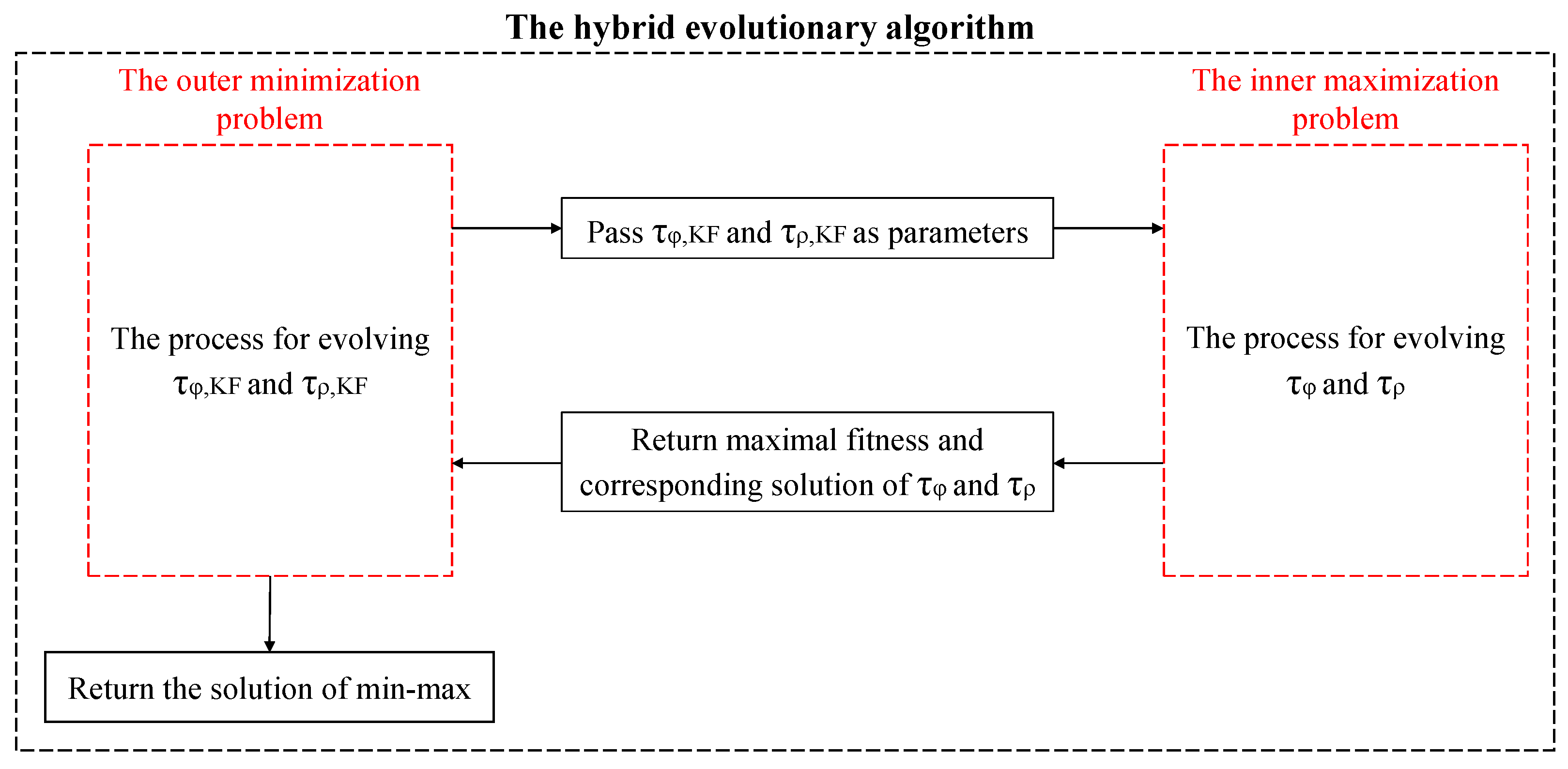
Until now, the bounding of the integrity risk and the reduction in conservatism for KF-based ARAIM have been transformed into solving Equation (16), which is composed of an inner maximization problem and an outer minimization problem. As mentioned before, gradient-based algorithms and the traditional evolutionary algorithm cannot be applied to the current min–max optimization problem due to several limitations. Therefore, a hybrid evolutionary algorithm with high efficiency is proposed as illustrated in Figure 1.

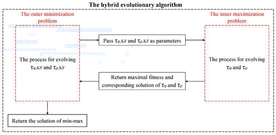
Figure 1. The framework of the whole process of the hybrid evolutionary algorithm.

In Figure 1, since ${\tau }_{\phi ,KF}$, ${\tau }_{\rho ,KF}$, ${\tau }_{\phi }$, and ${\tau }_{\rho }$ are for different optimal directions, i.e., the outer minimization and the inner maximization, ${\tau }_{\rho ,KF}$ and ${\tau }_{\phi ,KF}$ are evolved separately from ${\tau }_{\rho }$ and ${\tau }_{\phi }$. For each epoch in the KF time sequence, the hybrid evolutionary algorithm is used to find the minimum upper bound on the integrity risk. The processes for solving the inner maximization and outer minimization problems will be introduced separately later.

For the inner maximization problem, since it is easier and faster to optimize the unary function than the binary function, ${\tau }_{\rho }$ and ${\tau }_{\phi }$ are sequentially evolved, and the detailed steps are as follows:

Step 1: The population ${\mathrm{Pop}}_B$, which contains ${\tau }_{\rho }$, is initialized with equally spaced particles in the interval [10 s, 900 s]. The self-knowledge PSO is used to evolve ${\mathrm{Pop}}_B$, and only the first particle of ${\mathrm{Pop}}_B$ in the first generation is passed as the parameter to evolve ${\tau }_{\phi }$.

Step 2: When entering the process to evolve ${\tau }_{\phi }$, the population ${\mathrm{Pop}}_C$, which contains ${\tau }_{\phi }$, is also initialized with equally spaced particles. Then, the self-knowledge PSO is used where the fitness of each particle ${\tau }_{\phi }^i$ is calculated as being the value of $P_{HMI}({\tau }_{\phi }^i,{\tau }_{\rho },{\tau }_{\phi ,KF},{\tau }_{\rho ,KF}$) where ${\tau }_{\rho }$, ${\tau }_{\phi ,KF}$, and ${\tau }_{\rho ,KF}$ are frozen. The maximal fitness of each particle during all generations is regarded as the personal best solution. The output is the global best solution, which is the maximum among all personal best solutions.

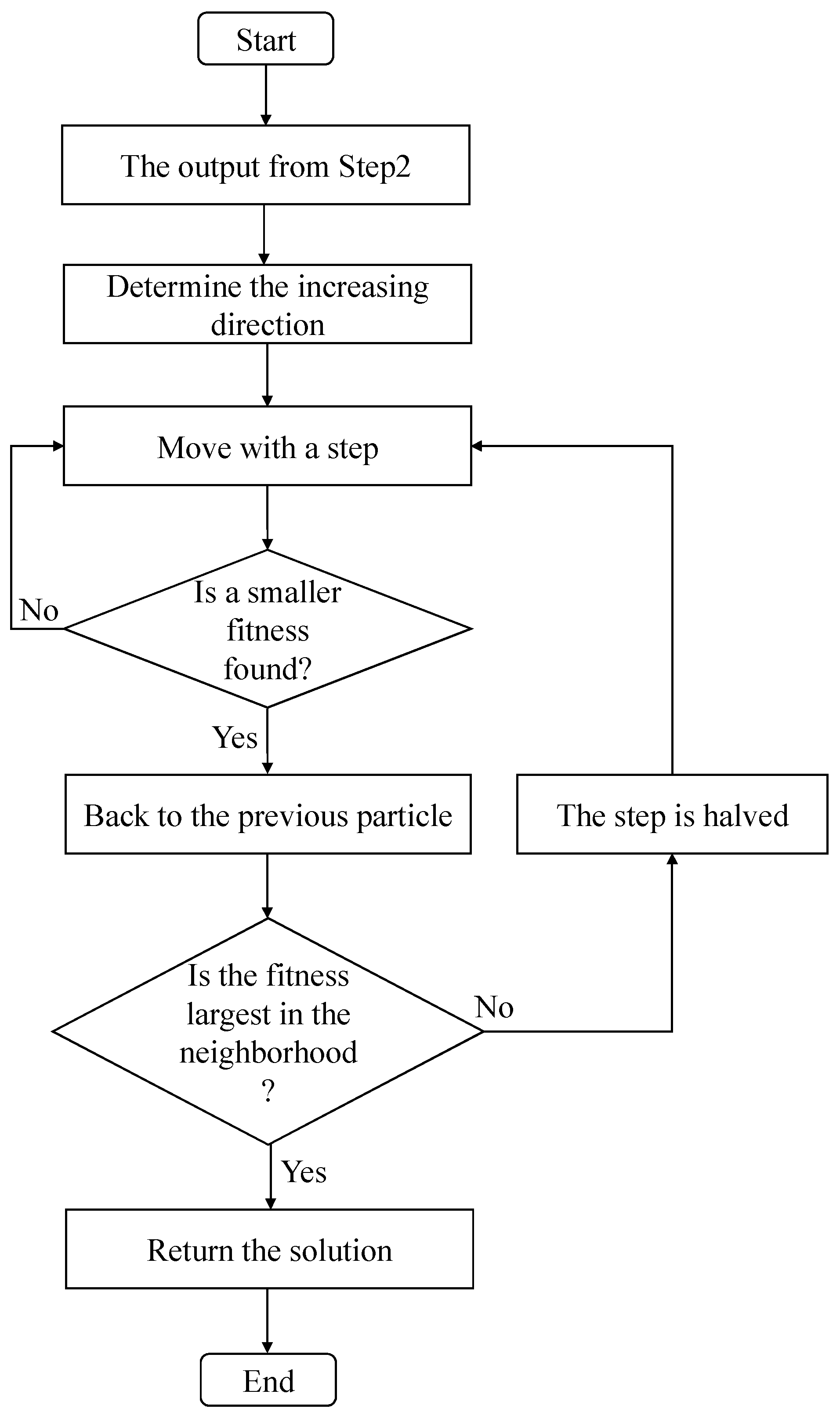
Step 3: By using the output from Step 2 as the initial value, the hill-climbing algorithm is used to quickly obtain the global best solution of ${\tau }_{\phi }$, which is shown in Figure 2. It first determines the increasing direction by calculating the fitness in the neighborhood of the initial value. Second, it moves to the increasing direction with an initial large step until a particle with the smaller fitness is found. Then, it backs to the previous particle and determines whether the fitness is largest in the neighborhood. If not, one half of the previous step is used to continue the process. Finally, the global best solution of ${\tau }_{\phi }$ is returned.

Figure 2. The hill-climbing algorithm.

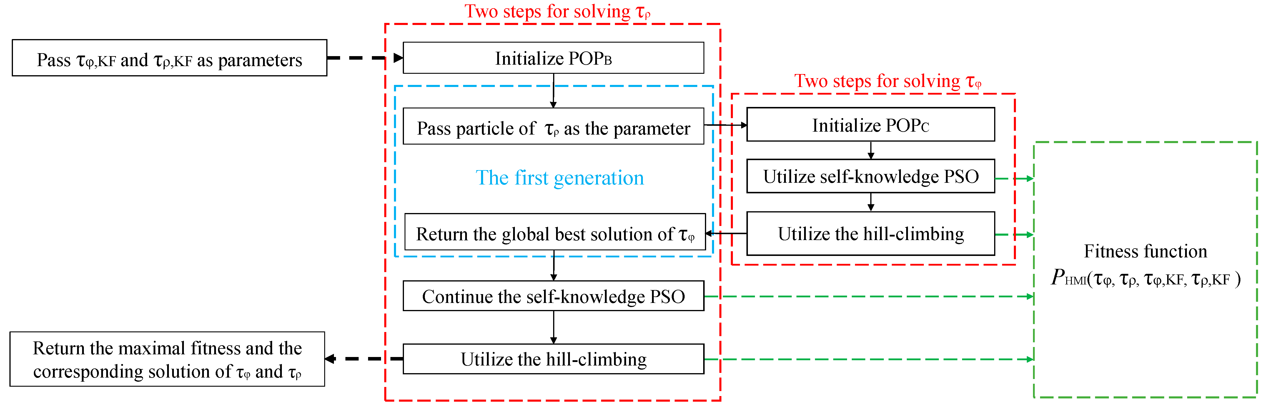
Step 4: When returning back to the process to evolve ${\tau }_{\rho }$, the self-knowledge PSO is continued, and then, the same hill-climbing is used as Step 3. Finally, the maximal fitness and the corresponding solution of ${\tau }_{\rho }$ and ${\tau }_{\phi }$ are returned. Figure 3 illustrates the whole process for solving the inner maximization problem.

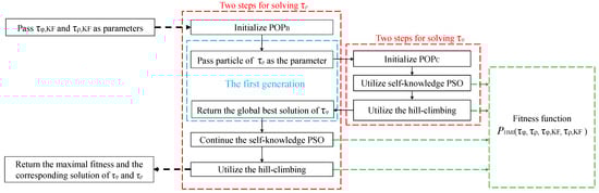
Figure 3. The framework of evolving ${\tau }_{\rho }$ and ${\tau }_{\phi }$ in the inner maximization problem.

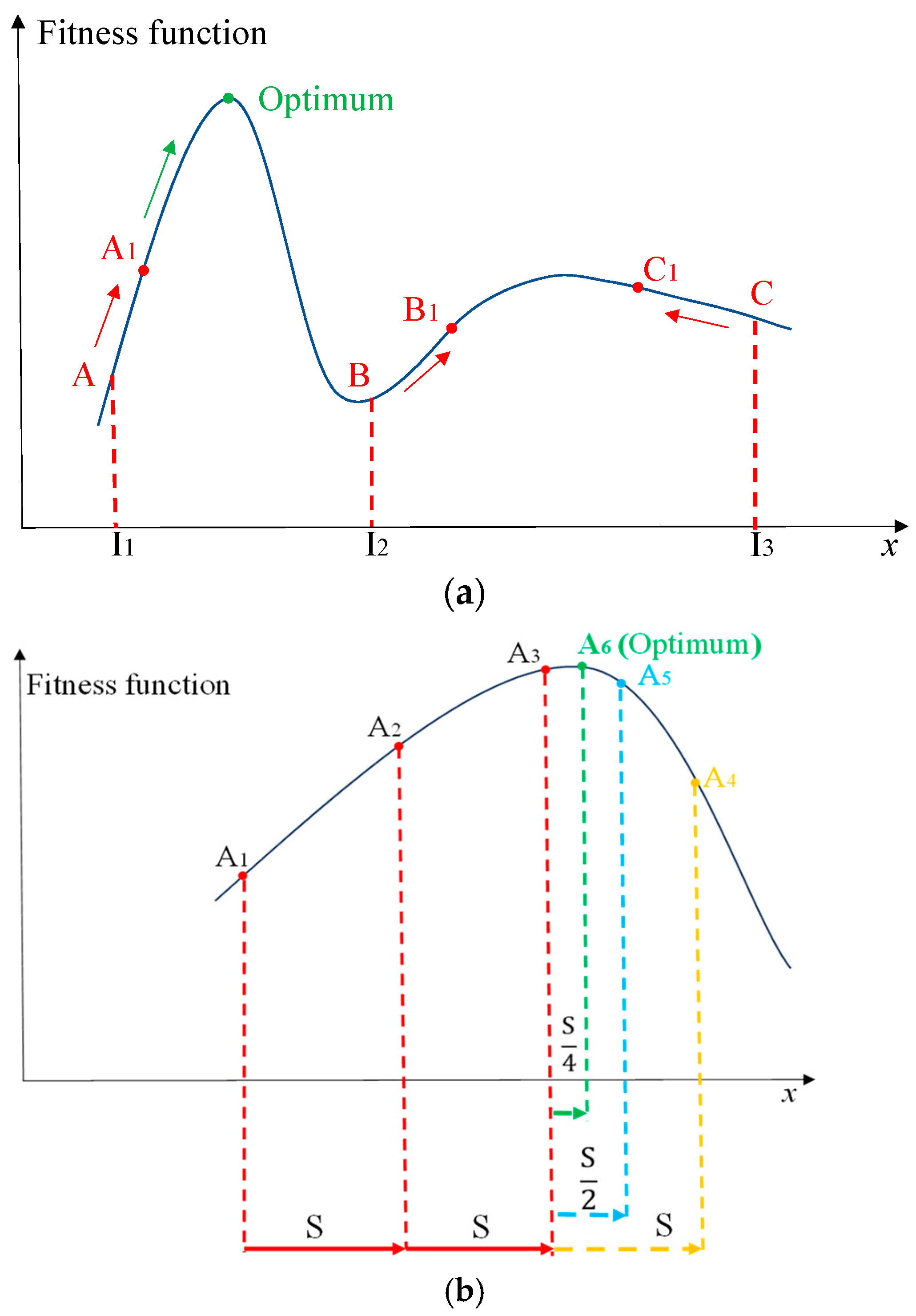
For convenience, the algorithm combining the self-knowledge PSO and the hill-climbing algorithm for solving the inner maximization problem is called SPSO-HC. More importantly, the principle of SPSO-HC is shown in Figure 4.

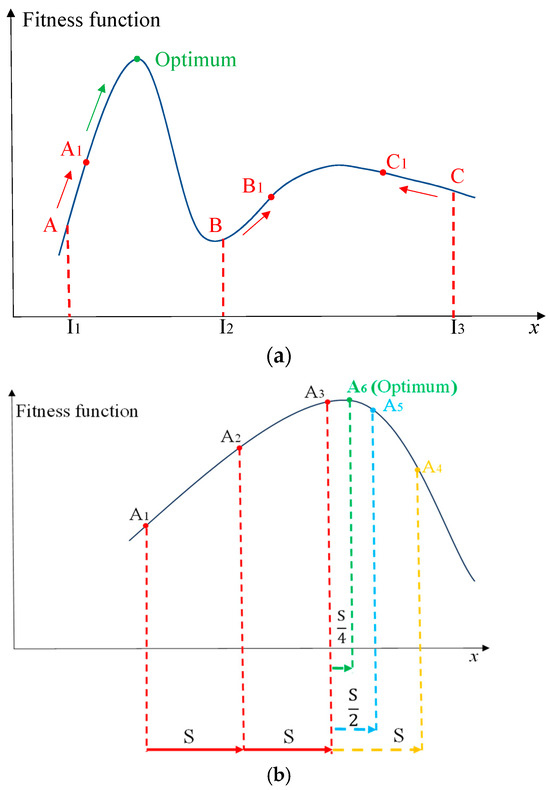
Figure 4. The principle of SPSO-HC. (a) Self-knowledge PSO algorithm; (b) hill-climbing algorithm.

In Figure 4a, I₁, I₂, and I₃ are initial values of three particles in the self-knowledge PSO where the velocity is updated by the inertia and cognition parts without the social part. After reaching the maximum number of generations, points A₁, B₁, and C₁ are the personal best points of each particle and the output is the global best point A₁ with the maximal fitness. The reason of removing the social part is to prevent points around global optimal area like point A from the interference of points around the local optimal area like point C. Since point C is larger than point A at the initial stage, if the standard PSO is used, a larger population and more generations are required to alleviate the effect of point C to obtain the global optimal solution.

Then, the hill-climbing algorithm uses point A₁ as the initial value and moves to the increasing direction with a large step $S$ as illustrated in Figure 4b. After three movements, the fitness of point A₄ is smaller than the fitness of point A₃. Then, the algorithm backs to A₃ and moves with one half of step, i.e., ${\displaystyle \frac{S}{2}}$. The fitness of point A₅ is still smaller than the fitness of point A₃. Once again, the algorithm backs to A₃ and moves with one half of the previous step, i.e., ${\displaystyle \frac{S}{4}}$, which finally obtains the global best point A₆ with the maximal fitness. By adaptively adjusting the step length, the hill-climbing algorithm can rapidly obtain the maximal value.

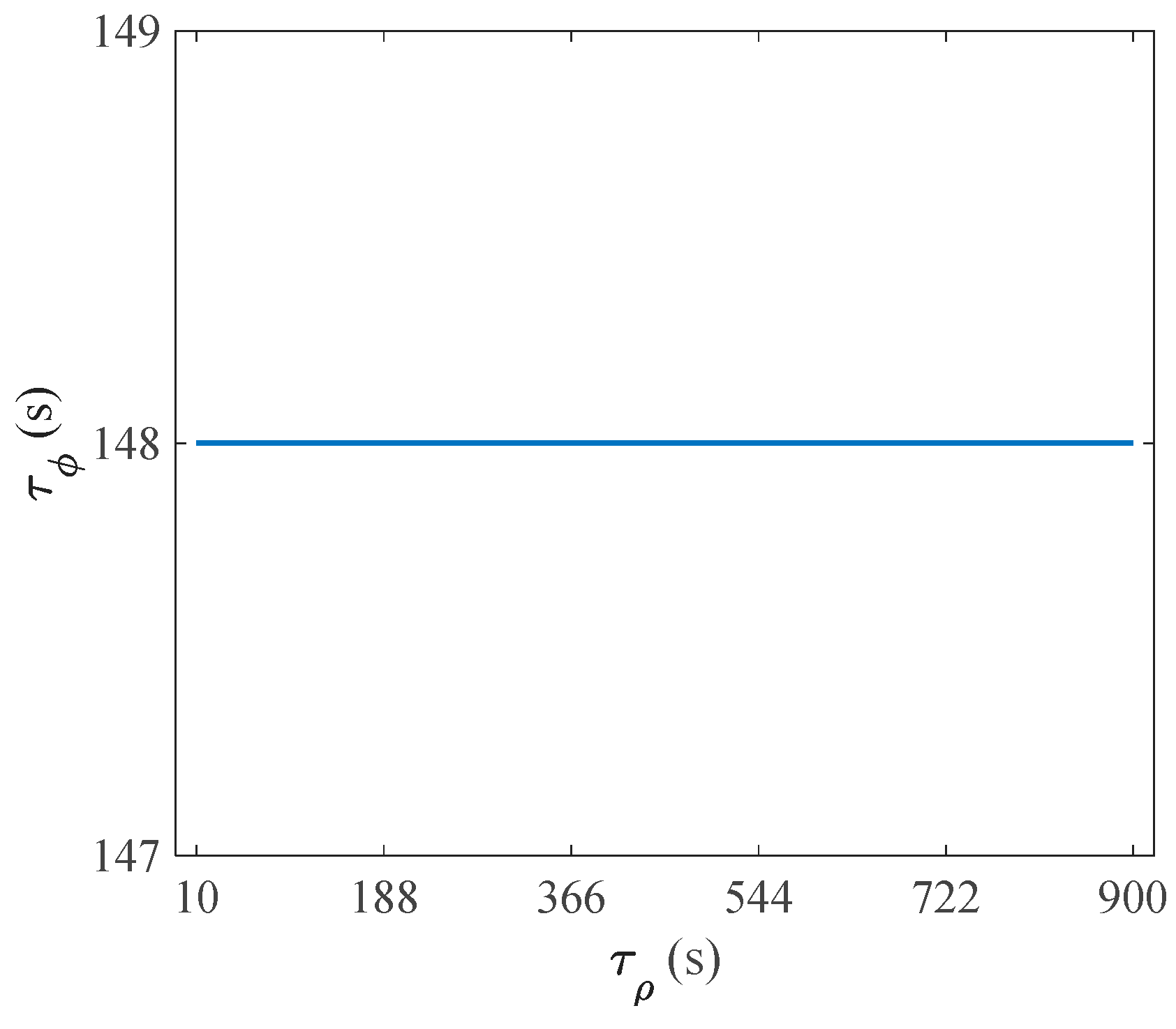
The self-knowledge PSO is for determining the global optimal area, and the hill-climbing algorithm is for finding the optimal solution rapidly in this local area. Moreover, the hill-climbing algorithm can ensure that the maximal solution is found; that is, the integrity risk is guaranteed to be bounded. In addition, the reason for only passing one particle of ${\mathrm{Pop}}_B$ in the first generation to evolve ${\tau }_{\phi }$ is analyzed in the following. The variation in ${\tau }_{\rho }$ cannot influence the global best solution of ${\tau }_{\phi }$ in the inner maximization problem, which is shown in Figure 5.

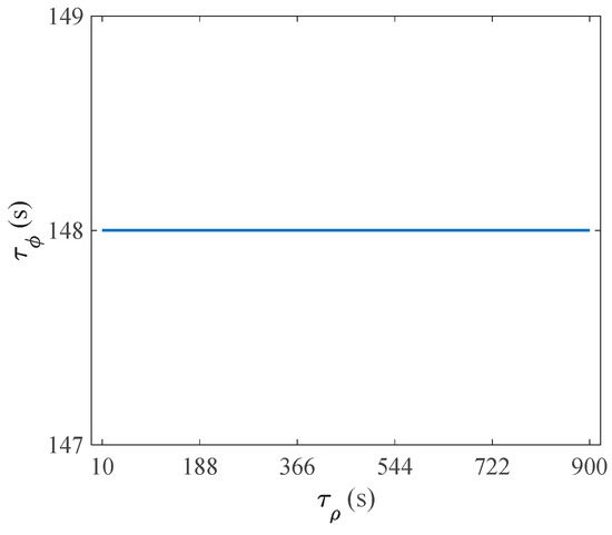
Figure 5. The global best solution of ${\tau }_{\phi }$ when ${\tau }_{\rho }$ is varied.

In Figure 5, the global best solution of ${\tau }_{\phi }$ is unchanged in the inner maximization problem when ${\tau }_{\rho ,KF}$ and ${\tau }_{\phi ,KF}$ are frozen, and ${\tau }_{\rho }$ is set to different values. Therefore, it only needs to determine the global best solution of ${\tau }_{\phi }$ once when evolving ${\tau }_{\rho }$; that is, only the first particle of ${\mathrm{Pop}}_B$ in the first generation is passed as the parameter to evolve ${\tau }_{\phi }$, which can save a lot of time.

To reduce conservatism with high efficiency in the outer minimization problem, the SPSO-HC is also used to evolve ${\tau }_{\rho ,KF}$ and ${\tau }_{\phi ,KF}$. As for the fitness function, the input is the particle containing ${\tau }_{\rho ,KF}$ and ${\tau }_{\phi ,KF}$, and the output is the maximal $P_{HMI}$ and the corresponding solutions of ${\tau }_{\phi }$ and ${\tau }_{\rho }$.

6. Simulation Results

6.1. Verification of the Bounding Covariance

To verify the bounding covariance, a KF estimation example is used, where the sampling interval $\Delta t$ is 1 s and the true value of the state $x_k^{*}$ is 1 m. In the measurement equation, the first-order GMP $m_k$ is generated using a time constant $\tau$ of 300 s and a variance 1.1 ${\mathrm{m}}^2$. Thus, based on Equation (1), the measurement and process equations can be written as follows:

$$\begin{array}{c}\left[\begin{array}{c}{z}_k^j\\ z_k^r\\ z_k^t\end{array}\right]=\left[\begin{array}{c}0.6k\\ 0.04k\\ 0.06k\end{array}\begin{array}{c} 1\\ 1\\ 1\end{array}\right]\left[\begin{array}{c}{x}_k^{*}\\ m_k\end{array}\right]+\left[\begin{array}{c}{n}_k^j\\ n_k^r\\ n_k^t\end{array}\right]\\ \left[\begin{array}{c}{x}_{k+1}^{*}\\ m_{k+1}\end{array}\right]=\left[\begin{array}{cc}1& 0\\ 0& e^{-{\displaystyle \frac{1}{\tau }}}\end{array}\right]\left[\begin{array}{c}{x}_k^{*}\\ m_k\end{array}\right]+\left[\begin{array}{c}0\\ {\eta }_k\end{array}\right]\end{array},$$

(19)

where $z_k^j$, $z_k^r$, and $z_k^t$ are different measurements at time $k$; $\left[\begin{array}{c}0.6k\\ 0.04k\\ 0.06k\end{array}\begin{array}{c} 1\\ 1\\ 1\end{array}\right]$ represents the observation matrix, which is changed with time; $\left[\begin{array}{c}{n}_k^j\\ n_k^r\\ n_k^t\end{array}\right]$ is zero-mean normally distributed and its covariance matrix is $\left[\begin{array}{ccc}{0.8}^2& 0& 0\\ 0& {0.8}^2& 0\\ 0& 0& {0.8}^2\end{array}\right]$; ${\eta }_k=\sqrt{{1.2}^2(1-e^{-{\displaystyle \frac{2\Delta t}{\tau }}})}{\mathsf{\zeta }}_k$ and ${\zeta }_k~N\left(0,1\right)$.

In the estimation process, the true correlation time constant is assumed to be unknown but lies within the interval [20 s, 400 s]. The state vector is initialized with 0 m, and the initial error covariance matrix is diagonal with two elements, i.e., $\left[\begin{array}{cc}1·{10}^6& 0\\ 0& 1·{10}^{-2}\end{array}\right]$. To illustrate the effect of the uncertainty correlation time constant on the variance, Sequential Monte Carlo (SMC) simulation, i.e., the particle filter, is used to obtain the true covariance [42]. For the standard covariance obtained from the KF, the correlation time constant is set to 20 s by the designer. As for the bounding covariance, the subset that excludes the first element $z_k^j$ is used to calculate the subset variance corresponding to $i$ = 1. The result is shown in Figure 6.

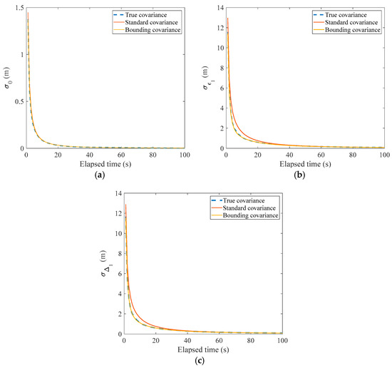
Figure 6. ${\sigma }_0$, ${\sigma }_{{\epsilon }_1}$, and ${\sigma }_{{\Delta }_1}$ from the true, standard, and bounding covariances. (a) ${\sigma }_0$; (b) ${\sigma }_{{\epsilon }_1}$; (c) ${\sigma }_{{\Delta }_1}$.

In Figure 6, the blue dashed, red, and yellow lines represent three standard deviations obtained from true, standard, and bounding covariances, respectively. Obviously, the red line is away from the blue dashed line, especially for ${\sigma }_{{\epsilon }_1}$ and ${\sigma }_{{\Delta }_1}$, which indicates that an imprecise correlation time constant can cause a significant difference in the variance. Since ${\sigma }_0$ is much smaller than ${\sigma }_{{\epsilon }_1}$ and ${\sigma }_{{\Delta }_1}$, its difference is smaller. Additionally, the standard deviation from the bounding covariance can match the true value. It is concluded that the effect of the uncertainty on the variance can be bounded through the bounding covariance as long as the true correlation time constant is known.

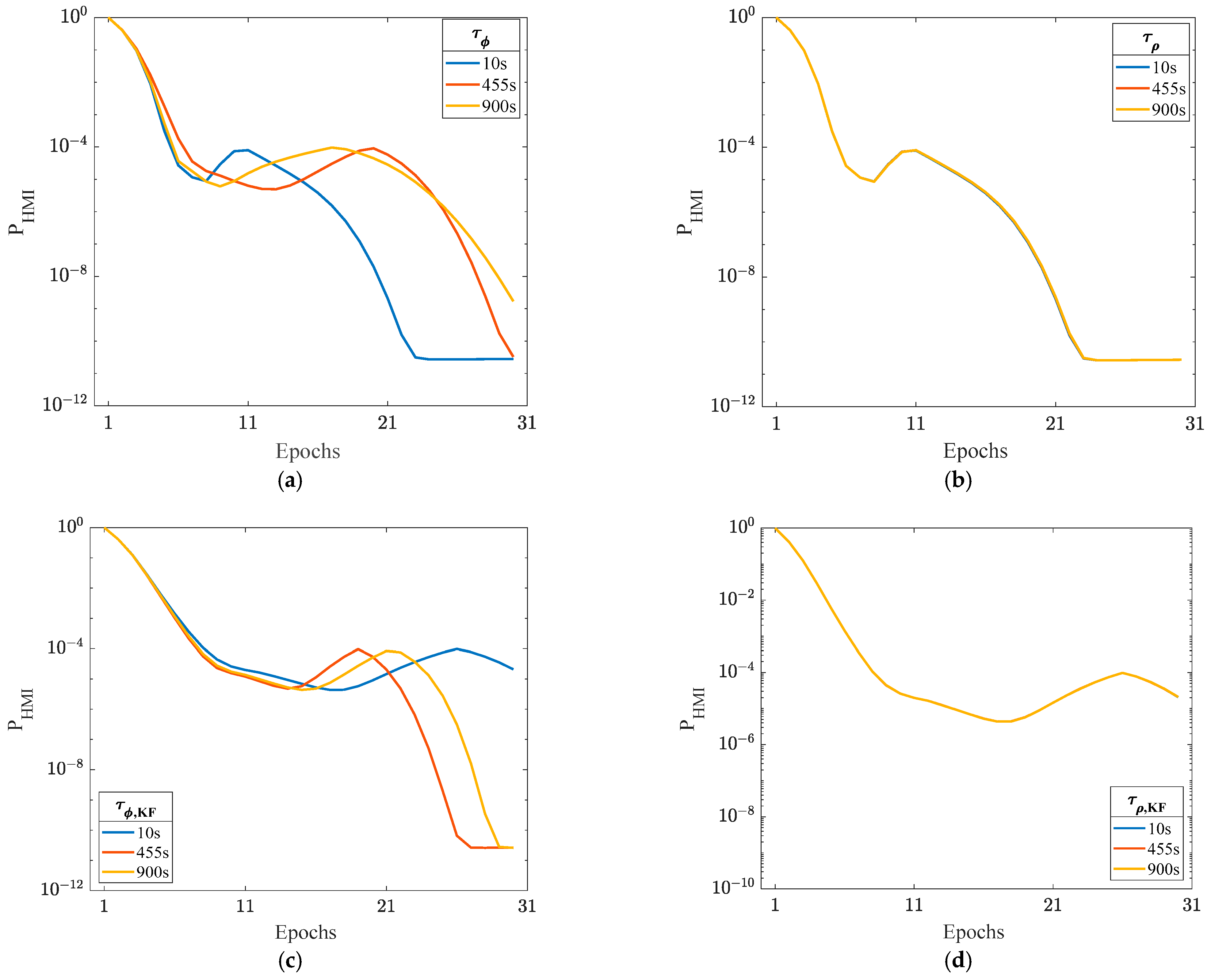
To further investigate the effects of variations in the correlation time constant on $P_{HMI}$, the following experiment is conducted. This experiment utilizes the GPS and BDS constellations [43,44] and the integrity risk is evaluated at HKSC station. Additionally, the simulation parameters are defined as follows [4]. The continuity risk requirement is 3.9 × 10⁻⁶ per approach, and the vertical alert limit is 35 m. The prior probabilities of single satellite fault and constellation fault are 10⁻⁵ and 10⁻⁴, respectively. The satellite elevation mask is 5°. In Figure 7a,b, ${\tau }_{\rho ,KF}$ and ${\tau }_{\phi ,KF}$ are fixed at 300 s while one of ${\tau }_{\rho }$ and ${\tau }_{\phi }$ is set to 10 s and the other is set to 10 s, 455 s, and 900 s. Similarly, ${\tau }_{\rho }$ and ${\tau }_{\phi }$ are fixed at 300 s, while one of ${\tau }_{\rho ,KF}$ and ${\tau }_{\phi ,KF}$ is set to 10 s and the other is set to 10 s, 455 s, and 900 s, which is shown in Figure 7c,d.

Figure 7. The different effects of the variation in four correlation time constants. (a) Variation in ${\mathsf{\tau }}_{\mathsf{\phi }}$; (b) variation in ${\tau }_{\rho }$; (c) variation in ${\tau }_{\phi ,KF}$; (d) variation in ${\tau }_{\rho ,KF}$.

As shown in Figure 7, it is obvious that variations in the carrier correlation time constants, i.e., ${\tau }_{\phi }$ and ${\tau }_{\phi ,KF}$, have a significant influence on $P_{HMI}$, while the effect of the variation in code correlation time constants, i.e., ${\tau }_{\rho }$ and ${\tau }_{\rho ,KF}$, is small. The reason for this is that the standard deviation of the code receiver noise is larger than that of the carrier. In Figure 7a,c, it is observed that ${\tau }_{\phi }$ and ${\tau }_{\phi ,KF}$ with the maximum integrity risk vary at different epochs; that is, fixed correlation time constants cannot guarantee the bounding of the integrity risk over all epochs. In addition, Figure 7a,c also show that using upper or lower values of correlation time constants cannot bound the integrity risk.

6.2. Comparison of Algorithms

To validate the SPSO-HC, two other EAs including the GA [45] and the standard PSO [46] are used to solve the inner maximization problem, i.e., $\max P_{HMI}\left({\tau }_{\phi },{\tau }_{\rho },{\tau }_{\phi ,KF},{\tau }_{\rho ,KF}\right)\{\begin{array}{c}{\tau }_{\phi ,KF}=10\\ {\tau }_{\rho ,KF}=10\\ 10\le {\tau }_{\rho }\le 900\\ 10\le {\tau }_{\phi }\le 900\end{array}$. For this maximization problem, the true solutions of ${\tau }_{\phi }$ and ${\tau }_{\rho }$ are 25 s and 900 s, as obtained using the brute-force searching method. The population size and the number of generations are set to 90 for the GA and 50 for the standard PSO. These algorithms are coded in MATLAB 2020a and run on a desktop computer with an Intel Core i9-10900K CPU (Intel Corpoartion, Santa Clara, CA, USA) @3.70 GHz and 128 GB of RAM in the 64-bit Windows 10 operating system. Additionally, each algorithm is run fifty times, and the result is illustrated in Table 1.

Table 1. Results using the GA, PSO, and SPSO-HC for the inner maximization problem.

Algorithm	Average Time (s)	Successful Run (%)
GA	484.43	56
PSO	154.67	64
SPSO-HC	2.39	100

In Table 1, the column “Successful Run (%)” indicates the percentage of the result of the algorithm when it is the same as the true solutions. It is obvious that SPSO-HC is much better than the GA, and the standard PSO from the perspective of stability and efficiency indicating the integrity risk is guaranteed to be bounded. It should be mentioned that if the population size and the number of generations increase, the percentage of successful run can be 100% for the GA and standard PSO but with a larger average time.

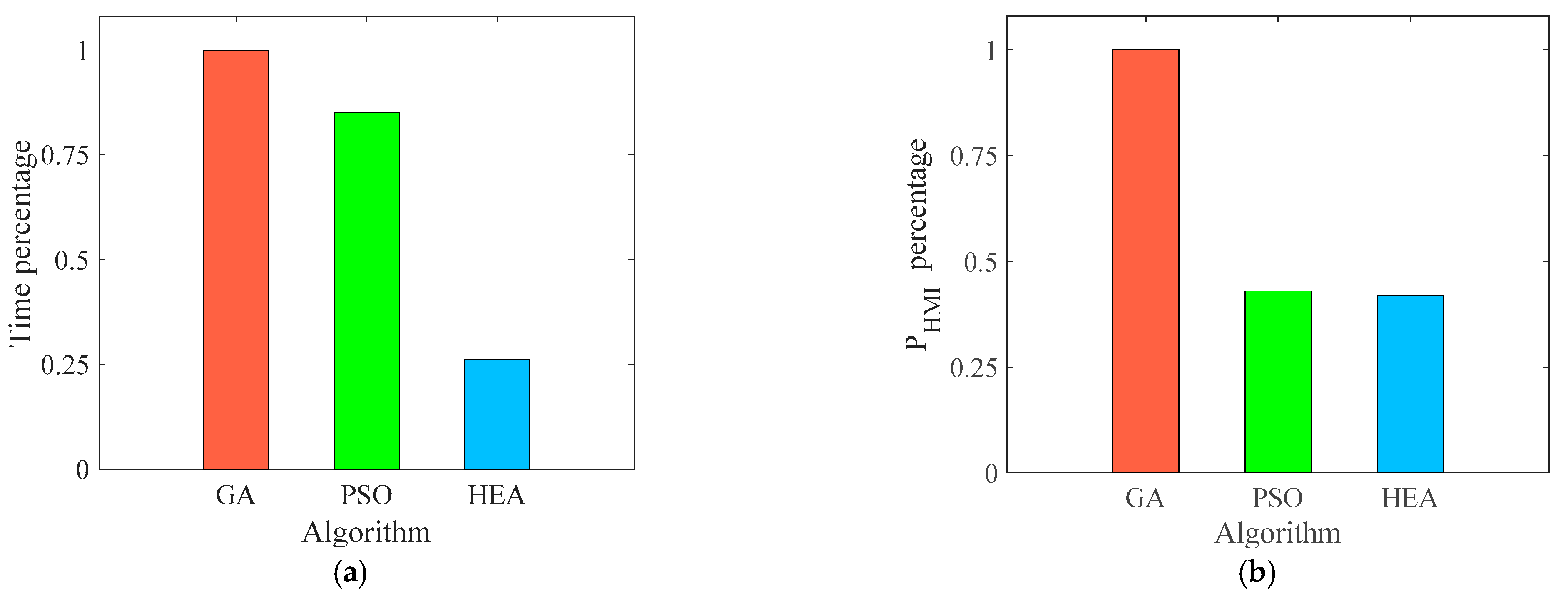
For comparison, the GA and the standard PSO are used to solve the outer problem where the inner problem is still solved by the SPSO-HC. To clearly observe the advantage of the proposed algorithm, two perspectives of the result, i.e., the time consumption and the evaluation of the integrity risk, are compared, as shown in Figure 8. It includes the time percentage and $P_{HMI}$ percentage, which are defined as the result from PSO and the hybrid evolutionary algorithm divided by the corresponding result from the GA. In particularly, the length of the bar of the GA is one since the result from the GA divided by itself is equal to one.

Figure 8. Comparison of three algorithms. (a) Time; (b) $P_{HMI}$.

In Figure 8, HEA represents the hybrid evolutionary algorithm. In Figure 8b, the blue bar is slightly shorter than the green bar indicating the HEA can obtain the smallest $P_{HMI}$. Obviously, the time consumption of the HEA is much less than PSO and the GA, as shown in Figure 8a. Thus, the smallest $P_{HMI}$ is obtained by the hybrid evolutionary algorithm in the shortest time; that is, the proposed algorithm can obtain the minimum upper bound on $P_{HMI}$ at the fastest speed. In short, the hybrid evolutionary algorithm is capable of solving the min–max problem, which only needs less than one minute to simultaneously bound the integrity risk and reduce conservatism at one epoch. Additionally, the proposed algorithm holds potential for extension to other scenarios, which needs to be investigated in the future work.

7. Conclusions

A method has been developed to overbound the model uncertainty in the time-correlated error for KF-based ARAIM when the time constant of the first-order GMP is known to lie within a specified interval. First, this work provides a new derivation of the recursive equation for two variances, i.e., the subset estimated error variance and the variance in the difference between the all-in-view solution and the subset solution, which is used to establish a direct mathematical expression that connects the integrity risk and the correlation time constant. Then, based on the obtained expression of the integrity risk, the min–max model is built to guarantee the bounding of the integrity risk and reduce conservatism at the same time. To rapidly solve the min–max optimization problem, a hybrid evolutionary algorithm is proposed where SPSO-HC conducts the global searching followed by the local searching. Specifically, in the SPSO-HC, the self-knowledge PSO first determines the local area of the global optimal solution, and then, the hill-climbing rapidly finds the optimal solution in this local area to guarantee the bounding of the integrity risk.

In the simulation for the inner problem, the SPSO-HC can achieve a 100% successful run with only a 2.39 s average time, performing much better compared with the GA and the standard PSO from the perspective of stability and efficiency. For the min–max optimization, the results show that the smallest $P_{HMI}$ is obtained by the hybrid evolutionary algorithm in the shortest time; that is, the proposed algorithm can obtain the minimum upper bound on $P_{HMI}$ at the fastest speed.

References

- Walter, T.; Blanch, J.; Gunning, K.; Joerger, M.; Pervan, B. Determination of fault probabilities for ARAIM. IEEE Trans. Aerosp. Electron. Syst. 2019, 55, 3505–3516. [Google Scholar] [CrossRef]
- Blanch, J.; Walter, T.; Enge, P.; Lee, Y.; Pervan, B.; Rippl, M.; Spletter, A.; Kropp, V. Baseline advanced RAIM user algorithm and possible improvements. IEEE Trans. Aerosp. Electron. Syst. 2015, 51, 713–732. [Google Scholar] [CrossRef]
- Dautermann, T. Extending required navigation performance to include time based operations and the vertical dimension. J. Inst. Navig. 2016, 63, 53–64. [Google Scholar] [CrossRef]
- Joerger, M.; Pervan, B. Multi-constellation ARAIM exploiting satellite motion. Navigation 2020, 67, 235–253. [Google Scholar] [CrossRef]
- Joerger, M.; Pervan, B. Exploiting satellite motion in ARAIM: Measurement error model refinement using experimental data. In Proceedings of the 29th International Technical Meeting of the Satellite Division of the Institute of Navigation, Portland, OR, USA, 12–16 September 2016. [Google Scholar]
- Tanil, C.; Khanafseh, S.; Joerger, M.; Pervan, B. Sequential integrity monitoring for Kalman filter innovations-based detectors. In Proceedings of the 31st International Technical Meeting of the Satellite Division of the Institute of Navigation, Miami, FL, USA, 24–28 September 2018. [Google Scholar]
- Li, Q.; Li, R.; Ji, K.; Dai, W. Kalman Filter and Its Application. In Proceedings of the 2015 8th International Conference on Intelligent Networks and Intelligent Systems (ICINIS), Tianjin, China, 1–3 November 2015. [Google Scholar] [CrossRef]
- Dhongade, A.P.; Khandekar, M.A. GPS and IMU Integration on an autonomous vehicle using Kalman filter (LabView Tool). In Proceedings of the 2019 International Conference on Intelligent Computing and Control Systems (ICCS), Madurai, India, 15–17 May 2019. [Google Scholar] [CrossRef]
- Polotski, V.; Kenne, J.P.; Gharbi, A. Kalman filter based production control of a failure-prone single-machine single-product manufacturing system with imprecise demand and inventory information. J. Manuf. Syst. 2020, 56, 558–572. [Google Scholar] [CrossRef]
- Fronckova, K.; Slaby, A. Kalman Filter Employment in Image Processing. In Proceedings of the Computational Science and Its Applications—ICCSA 2020: 20th International Conference, Cagliari, Italy, 1–4 July 2020. [Google Scholar] [CrossRef]
- Wan, E.A.; Van Der Merwe, R. The unscented Kalman filter for nonlinear estimation. In Proceedings of the IEEE 2000 Adaptive Systems for Signal Processing, Communications, and Control Symposium (Cat. No. 00EX373), Lake Louise, AB, Canada, 1–4 October 2000. [Google Scholar] [CrossRef]
- Joerger, M.; Pervan, B. Kalman filter-based integrity monitoring against sensor faults. J. Guid. Control Dyn. 2013, 36, 349–361. [Google Scholar] [CrossRef]
- Groves, P.D. Principles of GNSS, inertial, and multisensor integrated navigation systems, 2nd edition [Book review]. Ind. Robot. Int. J. 2015, 30, 26–27. [Google Scholar] [CrossRef]
- Miller, C.; O’Keefe, K.; Gao, Y. Time correlation in GNSS positioning over short baselines. J. Surv. Eng. 2012, 138, 17–24. [Google Scholar] [CrossRef]
- BrysonJR, A.E.; Henrikson, L.J. Estimation using sampled data containing sequentially correlated noise. J. Spacecr. Rocket. 1968, 5, 662–665. [Google Scholar] [CrossRef]
- Petovello, M.G.; O’Keefe, K.; Lachapelle, G.; Cannon, M.E. Consideration of time-correlated errors in a Kalman filter applicable to GNSS. J. Geod. 2009, 83, 51–56. [Google Scholar] [CrossRef]
- Gao, Y.; Jiang, Y.; Gao, Y.; Huang, G. A linear Kalman filter-based integrity monitoring considering colored measurement noise. GPS Solut. 2021, 25, 1–13. [Google Scholar] [CrossRef]
- Crespillo, O.G.; Langel, S.; Joerger, M. Tight Bounds for Uncertain Time-Correlated Errors With Gauss-Markov Structure in Kalman Filtering. IEEE Trans. Aerosp. Electron. Syst. 2023, 59, 347–4362. [Google Scholar] [CrossRef]
- Simon, D. Optimal State Estimation: Kalman, H Infinity, and Nonlinear Approaches, 1st ed.; John Wiley & Sons, Inc.: Hoboken, NJ, USA, 2006. [Google Scholar]
- Langel, S.; Khanafseh, S.; Pervan, B. Bounding integrity risk subject to structured time correlation modeling uncertainty. In Proceedings of the 2012 IEEE/ION Position, Location and Navigation Symposium, Myrtle Beach, SC, USA, 23–26 April 2012. [Google Scholar] [CrossRef]
- Langel, S.; Khanafseh, S.; Pervan, B. Bounding Integrity Risk for Sequential State Estimators in the Presence of Stochastic Modeling Uncertainty. In Proceedings of the AIAA Guidance, Navigation, and Control (GNC) Conference, Boston, MA, USA, 19–22 August 2013. [Google Scholar] [CrossRef]
- Langel, S.; Khanafseh, S.; Pervan, B. Bounding integrity risk for sequential state estimators with stochastic modeling uncertainty. J. Guid. Control Dyn. 2014, 37, 36–46. [Google Scholar] [CrossRef]
- Jada, S.K.; Joerger, M. GMP-overbound parameter determination for measurement error time correlation modeling. In Proceedings of the International Technical Meeting of the Institute of Navigation, San Diego, CA, USA, 21–24 January 2020. [Google Scholar]
- Langel, S.; Crespillo, O.G.; Joerger, M. A new approach for modeling correlated Gaussian errors using frequency domain overbounding. In Proceedings of the 2020 IEEE/ION Position, Location and Navigation Symposium (PLANS), Portland, OR, USA, 20–23 April 2020. [Google Scholar] [CrossRef]
- Tupysev, V.A.; Stepanov, O.A.; Loparev, A.V.; Litvinenko, Y.A. Guaranteed estimation in the problems of navigation information processing. In Proceedings of the 2009 IEEE Control Applications, (CCA) & Intelligent Control, (ISIC), St. Petersburg, Russia, 8–10 July 2009. [Google Scholar] [CrossRef]
- Langel, S.; Crespillo, O.G.; Joerger, M. Bounding sequential estimation errors due to Gauss-Markov noise with uncertain parameters. In Proceedings of the 32nd International Technical Meeting of the Satellite Division of the Institute of Navigation, Miami, FL, USA, 16–20 September 2019. [Google Scholar]
- Langel, S.; Crespillo, O.G.; Joerger, M. Overbounding the effect of uncertain Gauss-Markov noise in Kalman filtering. Navigation 2021, 68, 259–276. [Google Scholar] [CrossRef]
- Khanafseh, S.; Langel, S.; Pervan, B. Overbounding position errors in the presence of carrier phase multipath error model uncertainty. In Proceedings of the IEEE/ION Position, Location and Navigation Symposium, Indian Wells, CA, USA, 4–6 May 2010. [Google Scholar] [CrossRef]
- Rapoport, A.; Boebel, R.B. Mixed strategies in strictly competitive games: A further test of the minimax hypothesis. Games Econ. Behav. 1992, 4, 261–283. [Google Scholar] [CrossRef]
- Gohary, R.H.; Huang, Y.; Luo, Z.Q.; Pang, J.S. A generalized iterative water-filling algorithm for distributed power control in the presence of a jammer. IEEE Trans. Signal Process. 2009, 57, 2660–2674. [Google Scholar] [CrossRef]
- Arjovsky, M.; Chintala, S.; Bottou, L. Wasserstein generative adversarial networks. In Proceedings of the 34th International Conference on Machine Learning, Sydney, Australia, 6–11 August 2017. [Google Scholar]
- Razaviyayn, M.; Huang, T.; Lu, S.; Nouiehed, M.; Sanjabi, M.; Hong, M. Nonconvex min-max optimization: Applications, challenges, and recent theoretical advances. IEEE Signal Process. Mag. 2020, 37, 55–66. [Google Scholar] [CrossRef]
- Lin, T.; Jin, C.; Jordan, M. On gradient descent ascent for nonconvex-concave minimax problems. In Proceedings of the 37th International Conference on Machine Learning, Virtual Event, 13–18 July 2020. [Google Scholar]
- Vikhar, P.A. Evolutionary algorithms: A critical review and its future prospects. In Proceedings of the 2016 International Conference on Global Trends in Signal Processing, Information Computing and Communication (ICGTSPICC), Jalgaon, India, 22–24 December 2016. [Google Scholar] [CrossRef]
- Barbosa, H.J. A coevolutionary genetic algorithm for constrained optimization. In Proceedings of the 1999 Congress on Evolutionary Computation-CEC99 (Cat. No. 99TH8406), Washington, DC, USA, 6–9 July 1999. [Google Scholar] [CrossRef]
- Cramer, A.M.; Sudhoff, S.D.; Zivi, E.L. Evolutionary algorithms for minimax problems in robust design. IEEE Trans. Evol. Comput. 2008, 13, 444–453. [Google Scholar] [CrossRef]
- Shi, Y.; Krohling, R.A. Co-evolutionary particle swarm optimization to solve min-max problems. In Proceedings of the 2002 Congress on Evolutionary Computation. CEC’02 (Cat. No. 02TH8600), Honolulu, HI, USA, 12–17 May 2002. [Google Scholar] [CrossRef]
- Krohling, R.A.; Coelho, L.S. Coevolutionary particle swarm optimization using Gaussian distribution for solving constrained optimization problems. IEEE Trans. SMC Part B (Cybern.) 2006, 36, 1407–1416. [Google Scholar] [CrossRef]
- Segundo, G.A.; Krohling, R.A.; Cosme, R.C. A differential evolution approach for solving constrained min–max optimization problems. Expert Syst. Appl. 2012, 39, 13440–13450. [Google Scholar] [CrossRef]
- Pervan, B.; Khanafseh, S.; Patel, J. Test statistic auto-and cross-correlation effects on monitor false alert and missed detection probabilities. In Proceedings of the 2017 International Technical Meeting of the Institute of Navigation, Monterey, CA, USA, 30 January–2 February 2017. [Google Scholar]
- Daskalakis, C.; Skoulakis, S.; Zampetakis, M. The complexity of constrained min-max optimization. In Proceedings of the 53rd Annual ACM SIGACT Symposium on Theory of Computing, Virtual Event, 21–25 June 2021. [Google Scholar] [CrossRef]
- Gustafsson, F. Particle filter theory and practice with positioning applications. IEEE Trans. Aerosp. Electron. Syst. 2010, 25, 53–82. [Google Scholar] [CrossRef]
- MAAST for ARAIM Version 0.4. Available online: https://gps.stanford.edu/resources/software-tools/maast (accessed on 1 April 2022).
- Bai, S.; Zhang, Y.; Jiang, Y.; Sun, W.; Shao, W. Modified Two-Dimensional Coverage Analysis Method Considering Various Perturbations. IEEE Trans. Aerosp. Electron. Syst. 2024, 60, 2763–2777. [Google Scholar] [CrossRef]
- Lambora, A.; Gupta, K.; Chopra, K. Genetic algorithm-A literature review. In Proceedings of the 2019 International Conference on Machine Learning, Big Data, Cloud and Parallel Computing (COMITCon), Faridabad, India, 14–16 February 2019. [Google Scholar] [CrossRef]
- Wang, D.; Tan, D.; Liu, L. Particle swarm optimization algorithm: An overview. Soft Comput. 2018, 22, 387–408. [Google Scholar] [CrossRef]
Disclaimer/Publisher’s Note: The statements, opinions and data contained in all publications are solely those of the individual author(s) and contributor(s) and not of MDPI and/or the editor(s). MDPI and/or the editor(s) disclaim responsibility for any injury to people or property resulting from any ideas, methods, instructions or products referred to in the content. |
© 2024 by the authors. Licensee MDPI, Basel, Switzerland. This article is an open access article distributed under the terms and conditions of the Creative Commons Attribution (CC BY) license (https://creativecommons.org/licenses/by/4.0/).