Abstract
During the beam current calibration process, accurate guidance of the beam current to the metal target is a challenging issue for proton accelerators. To address this challenge, we propose the use of beam orbital parameters combined with reinforcement learning algorithms to achieve automatic beam calibration. This study introduces a system architecture that employs edge intelligent acceleration nodes based on deep learning acceleration techniques. We designed a system to predict BPM parameters using a cascaded backpropagation neural network (CBPNN) that is informed by the physical structure. This system serves as an environmental map for reinforcement learning, aiding beam current correction. The CBPNN was implemented on the acceleration node to hasten the forward inference process, leveraging sparsification, quantization algorithms, and pipelining techniques. Our experimental results demonstrated that the simulated inference speed reached 28 μs with FPGA hardware as the edge acceleration node, achieving forward inference speeds 35.66 and 12.66 times faster than those of the CPU and GPU. The energy efficiency ratio was 10.582 MOPS/W, which was 989 and 410 times that of the CPU and GPU, respectively. This confirms the designed architecture’s energy efficiency and low latency attributes.
1. Introduction
The China Initiative for Accelerator Driven System (CiADS) is a complex system that involves multiple fields, such as accelerator physics, magnetism, electricity, automatic control, and mechanical processing. Therefore, its beam trajectory is often affected by multiple factors, such as processing errors of equipment and components, misalignment of track centers, magnetic field interference, circuit noise, vacuum degree, measurement errors, control errors, etc., and it deviates from the predetermined track. This may cause beam loss and even lead to equipment failure and personnel injury [1]. In order to solve the problem, scientists have conducted extensive research and improved the beam offset situation and control accuracy through various means, such as theoretical analysis and empirical judgment. However, the beam offset problem is still quite serious. How to further solve the problem of beam offset and improve the quality of beam transmission remains a very important scientific issue of concern in the fields of accelerators and control at home and abroad.
The latest idea is to use deep learning algorithms to automatically correct the beam trajectory. For example, neural network-based beam trajectory parameter prediction and reinforcement learning-based beam trajectory offline correction aim to predict a set of control parameters in advance for the beam to operate on a predetermined trajectory before the accelerator is officially started [1]. These methods have laid the research foundation for the true implementation of beam correction. However, most of them are offline correction methods. Real-time correction control cannot be provided for beam track deflection that occurs during the operation of the beam. In addition, a single deep learning algorithm cannot achieve real-time correction of time-related beam trajectories. Therefore, in our previous work, we proposed a method for online correction of accelerator beam trajectories based on multi-agent reinforcement learning. The idea of this method is to divide the accelerator into several control units according to functional segments for separate control, thereby improving control accuracy while reducing control difficulty. For this purpose, we plan to deploy reinforcement learning in FPGA-based edge nodes to achieve edge intelligent nodes and utilize these intelligent nodes to achieve online control of accelerators, thereby achieving correction of beam trajectories.
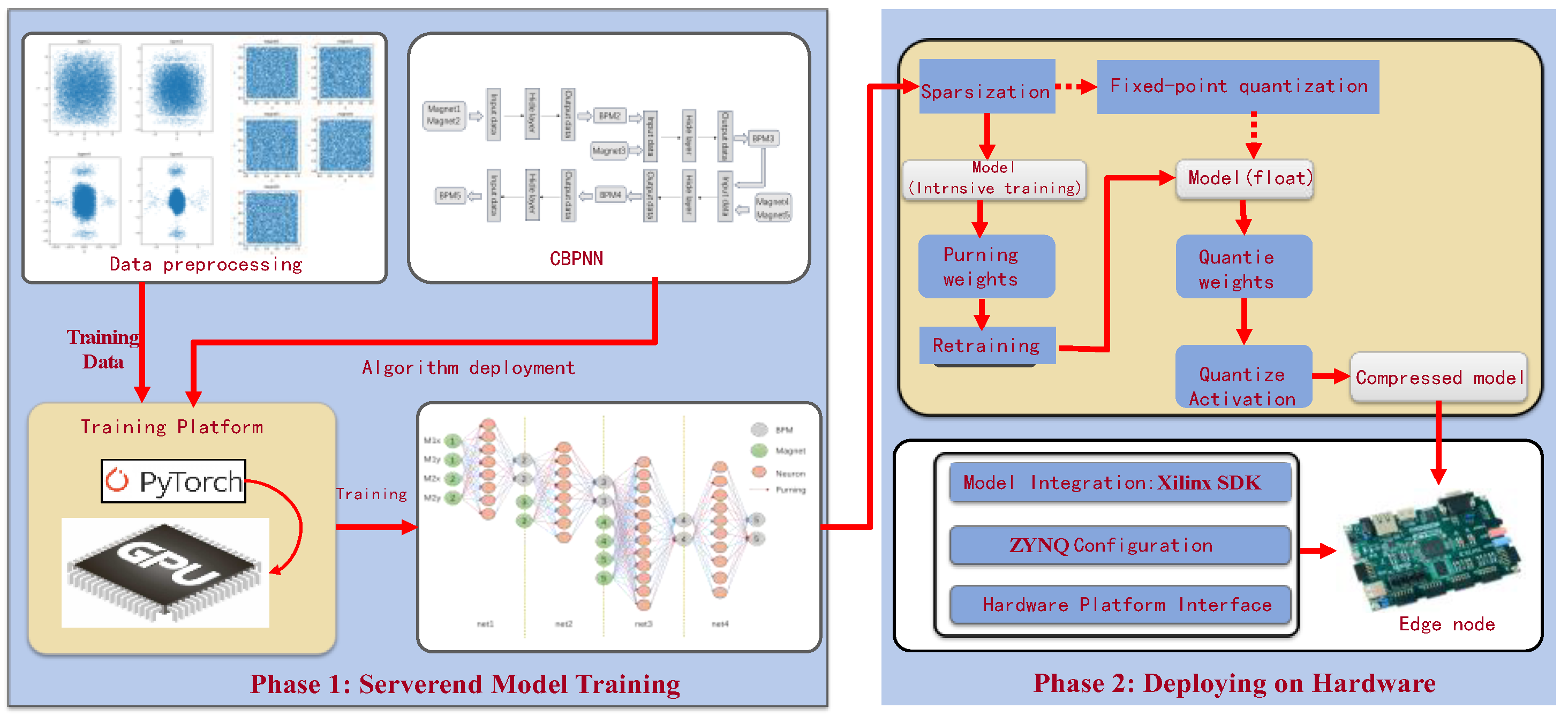
Based on the above research ideas, we evaluated a system solution for deploying reinforcement learning (RL) on the edge intelligence acceleration node framework. As part of the testing, we introduced CBPNN as an environment of RL that matches the physical structure of the medium energy beam transport line (MEBT) segment in a linear accelerator. This environment was deployed in the deployment framework of the designed deep learning edge intelligence acceleration node to verify the feasibility, low latency, and reliability of the system framework [2].
In order to efficiently embed deep learning algorithms into FPGA and achieve accelerator control systems based on edge intelligent computing, the deployment problem of CBPNN based on FPGA edge intelligent nodes was studied. Firstly, we studied a cascaded neural network (CBPNN) based on the characteristics of the MEBT accelerator environment. After training the optimal model, we attempted to achieve parallel acceleration of CBPNN in FPGAs through processes such as sparsification of network weights, weight quantization, parallel acceleration, and deployment. Then, a series of experiments were conducted to verify the feasibility and acceleration effect of the method. The results indicate that the method we adopted is very promising, and after further research, we can achieve accelerator beam correction based on edge intelligent nodes.
The structure of the paper is as follows: Section 1 introduces the background and significance of the work; Section 2 introduces the relevant work; Section 3 introduces the system architecture; Section 4 introduces the acceleration algorithm of the algorithm in FPGAs; Section 5 introduces the test results of the system and discusses them; Section 6 summarizes the entire text and provides prospects for future work.
2. Related Work
2.1. Current Status of Accelerator Beams Orbital Parameter Predictions
Numerous domestic and international research institutions and teams are actively studying the prediction of particle accelerator beam orbit parameters. A prominent example includes the Institute of Modern Physics (IMP) at the Chinese Academy of Sciences and CERN (European Organization for Nuclear Research). The efficient operation of particle accelerators depends significantly on understanding the kinetic behavior of the beam current during the acceleration process. This behavior is influenced by factors such as space charge effects, damping effects, collective effects, and nonlinear effects [3]. Various methods have been proposed for predicting the orbital parameters of the beam, with common orbital correction methods relying on MICADO and SVD algorithms. These algorithms are applied to response matrices, facilitating linear mappings for computing BPM from the response matrix and corresponding corrected iron intensity data.
In recent years, there has been an increasing amount of research using machine learning methods applied to the particle accelerator field. The machine learning approach is an artificial intelligence technique that employs artificial intelligence algorithms to analyze and learn patterns and knowledge from data to enable prediction and decision-making. This approach uses historical data to construct predictive models without relying on mathematical modeling. Its significant advantages include the ability to handle nonlinear and high-dimensional problems as well as strong fitting and adaptive capabilities. However, the method itself does not capture the inner workings and principles of phenomena and requires enormous amounts of high-quality data for training and validation. Researchers at SLAC have used machine learning methods to optimize the nonlinear problem of an electronic storage ring, searching for Pareto solutions for multi-objective optimization instead of the traditional multi-objective genetic algorithm and particle swarm algorithm [4]. Researchers at ALS Light have experimented with the use of machine learning algorithms to compensate for changes in the beam state caused by changes in the magnetic gap of the insert instead of the traditional feed-forward approach [5]. Chen X et al. proposed a reinforcement learning algorithm to control the accelerator beam trajectory and gradually realized the automatic control of the accelerator beam trajectory by training the reinforcement learning model in the simulation platform and the real system [6]. The feasibility of applying the reinforcement learning model in particle accelerator beam current correction was verified. As a result, we plan to deploy reinforcement learning algorithms in edge intelligent acceleration nodes to reduce the system latency and improve the efficiency of beam current correction.
2.2. Deep Learning Acceleration Technology
Nowadays, artificial intelligence has pervaded various sectors of society in the era of intelligence. As a prominent research branch of AI, the development and study of neural network-related technologies have become the driving force behind modern intelligence. With the continuous growth in the size of mainstream neural networks and the improvement in accuracy rates, correctly deploying these neural networks onto hardware platforms has become a focal point for researchers. Deep neural networks have demonstrated superiority over traditional algorithms in numerous domains [7].
However, the high computational requirements and memory footprint of these networks in applications and the increasing algorithmic complexity of various cloud-based tasks require the use of edge acceleration nodes to share the arithmetic pressure for servers. As a result, various edge acceleration deployment platforms have emerged, such as GPU- and FPGA-based platforms. GPUs provide efficient acceleration for deep neural networks and are relatively energy inefficient. On the other hand, FPGA-based deployments offer advantages in terms of reprogrammability, high energy efficiency ratio, and parallel acceleration. Using FPGAs as edge intelligent acceleration nodes can take full advantage of their high energy efficiency ratio and parallel acceleration to reduce the delayed response and energy consumption of the deployment of deep learning networks. Biookaghazadeh S. et al. used a multi-FPGA acceleration scheme to handle complex CNN tasks [8].
Current acceleration algorithms using FPGAs as edge acceleration nodes are also applied to different application contexts. Xia et al. accelerated the frequency of laser absorption spectroscopy stratigraphy imaging (LAST) using FPGAs [9]. Luo Y. et al. achieved real-time detection and identification of plant diseases by accelerating CNNs with FPGAs [10]. FPGA-accelerated design often encompasses several common neural network compression methods, such as deep compression techniques, including network pruning, model quantization, and knowledge distillation.
Deep learning has demonstrated superior performance compared to traditional algorithms in various domains. However, the significant volume of parameters in deep learning models necessitates compression and acceleration for their application on edge devices. Neural network pruning can significantly compress the model while maintaining accuracy. With the weight parameters reduced, the weight memory, which is implemented by the on-chip memory on FPGAs, allows for high-speed access to the memory [11]. Model quantization can map full-precision numbers (activation values, parameters, and even gradient values) to a finite integer space via a quantization function. Model quantization can reduce the storage space of each parameter, reduce the computational complexity, and thus achieve neural network acceleration. Markus Nagel et al. systematically introduced model quantization methods in A White Paper on Neural Network Quantization. The actual quantization acceleration effect also depends on whether the deployed hardware platform has relevant inference libraries [12]. Riadh Ayachi et al. summarized optimization methods such as data quantization, fast matrix computation, frequency optimization, optimized on-chip memory design, data paths, and loop unrolling [13]. Kuan Wang et al. proposed hardware-aware automatic quantization, which utilizes reinforcement learning to automatically determine the quantization strategy and effectively reduces the delay by 1.4 to 1.95 times and energy consumption by 1.9 times compared to fixed bit width [14]. Currently, although many quantization frameworks can perform automatic quantization for some general models, they are not individually optimized for specialized networks and special network linear layers, and quantization failures can occur in practice.
Currently, for FPGA deployment of deep learning networks, various FPGA companies have also developed a variety of convenient automated deployment tools, such as the FINN automated deployment tool developed by Xilinx, which was used to generate an HLS code by SA Alam et al. [15]. The HLS4ml tool developed by Columbia University, MIT, and other top universities in the United States was originally developed to address the needs related to the field of high-energy physics [16]. These frameworks still have some shortcomings in practical applications, such as the fact that dynamic quantized deployment for specific frameworks is still not supported. Due to the specificity of the sparsely trained neural network, the deployment of the network for the quantization framework as well as the automated tools is defective in the coordination. Therefore, in this study, the basic data quantization algorithms and self-programmed HLS file writing process were used to achieve good acceleration results.
2.3. Introduction to Cascade Backpropagation Neural Networks
Cascade neural network is a variant of neural network, which is composed of small sub-neural networks that gradually increase hidden layer units and finally form a multi-layer neural network. The partial output of its i-th sub-neural network is a partial input of its i + 1th sub-neural network (i ≥ 1). It has the characteristic of rapid deployment for specific applications. In this study, we used BPNN as a sub-neural network component to establish a cascaded neural network.
BPNN is a multi-layer feedforward neural network based on an error backpropagation algorithm. It consists of input, hidden, and output layers, and each layer can contain multiple neurons. The calculation process is divided into two stages: forward propagation and backward propagation. Its structure is shown in Figure 1. It can minimize the error between the network output and the expected output by adjusting the weights and thresholds of the network. It has excellent nonlinear mapping ability and flexible network structure, which can be applied in fields such as function approximation, pattern recognition, classification, and data compression [17,18]. In the actual neural network design of this study, we cascaded four BP neural networks combined with external inputs into a larger-scale neural network model, namely, the cascaded BP neural network (CBPNN).
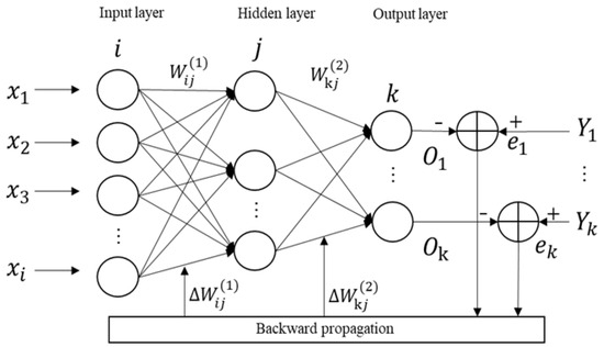
Figure 1.
BPNN architecture.
3. System Architecture and Methodological Design
3.1. Introduction to the Research Environment
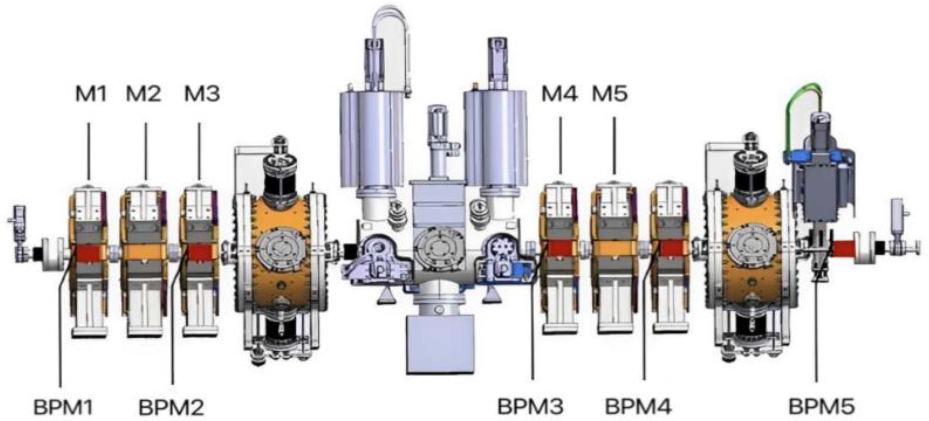
Our research is based on the MEBT segment of CiADS. MEBT is a crucial component of the C-ADS project, which is aimed at matching RFQ with the superconducting linear accelerator section, guiding the beam from RFQ, and outputting it correctly to the superconducting accelerator section. In the C-ADS Injector II system, the beam energy of RFQ is 2.1 MeV, and the sub-beam is an asymmetric beam. However, the superconducting half wavelength cavity requires a symmetric beam, and MEBT is required to complete this task. MEBT consists of six quadrupole magnets (M1, M2, …, M6), two beam concentrators (Buncher1 and Buncher2), one beam scraper (Scatter), one long drift segment (FC2), and several beam diagnostic elements. The layout of each component is shown in Figure 2.
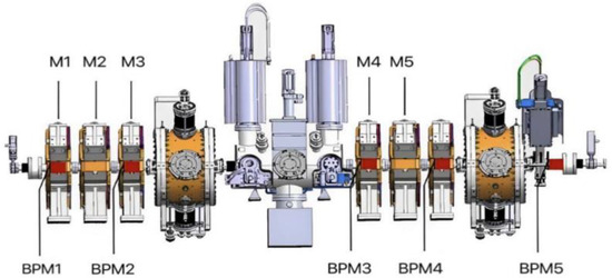
Figure 2.
Schematic diagram of the MEBT-segment structure of CAFe [6].
When the beam enters MEBT from RFQ, its position is first monitored by BPM1. Under the action of quadrupole magnets M1 and M2, the beam will be deflected (focused or defocused). BPM2 is placed between M2 and M3 to monitor the new position of the quantity, and it is then subjected to the action of the quadrupole magnet M3 and the scraper. Next, the beam is longitudinally focused by the beam splitter Buncher1. BPM3 can then monitor the new position of the beam, and under the action of quadrupole magnets M4 and M5, the beam will be deflected again. BPM4 can monitor the new position of the beam, and under the action of the quadrupole magnet M6 and the scraper, the beam will be deflected again. BPM5 can monitor the new position of the beam. The new bit value is then longitudinally focused by the beam splitter Buncher2 and output into the superconducting cavity.
3.2. Introduction to Beam Track Correction Algorithm
In our previous research work, we designed a multi-agent reinforcement learning algorithm to predict control parameters of neural networks online, executed the reinforcement learning control algorithm using MEBT, and used the output BPM value as input to the multi-agent reinforcement learning algorithm. In order to simulate the beam operation environment of MEBT, we designed a CBPNN and combined it with subsequent multi-agent reinforcement learning algorithms to complete beam correction. The interaction diagram between a single agent and the system is shown in Figure 3.
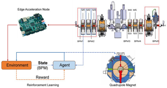
Figure 3.
Schematic diagram of interaction between intelligent agents and the system environment.
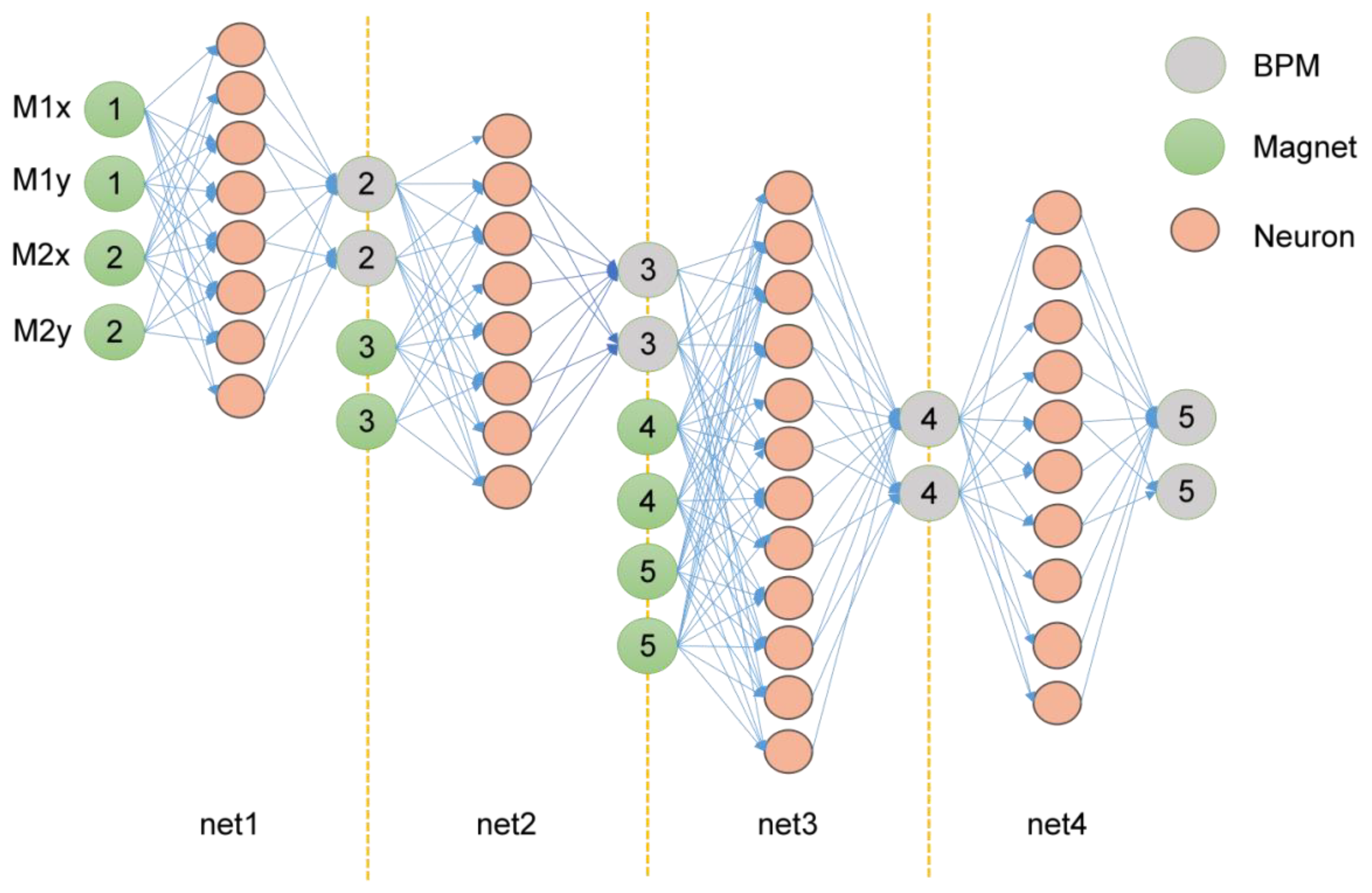
In the system design, BPNN was used as a sub-network form of cascaded neural network, and four BPNN were designed to represent four groups of magnets. By cascading four BPNN, CBPNN was implemented to simulate the beam-running environment of MEBT. The input of each level of the neural network is the control parameters of the magnet, and the output is the BPM of the beam current. On the contrary, the multi-agent reinforcement learning algorithm we designed is used to generate control strategies to control the parameters of the quadrupole magnet. Its input is BPM, and its output is the magnet control parameters for the next stage. CBPNN and multi-agent reinforcement learning algorithms form a complete closed loop, simulating the entire operation and control process of MEBT.
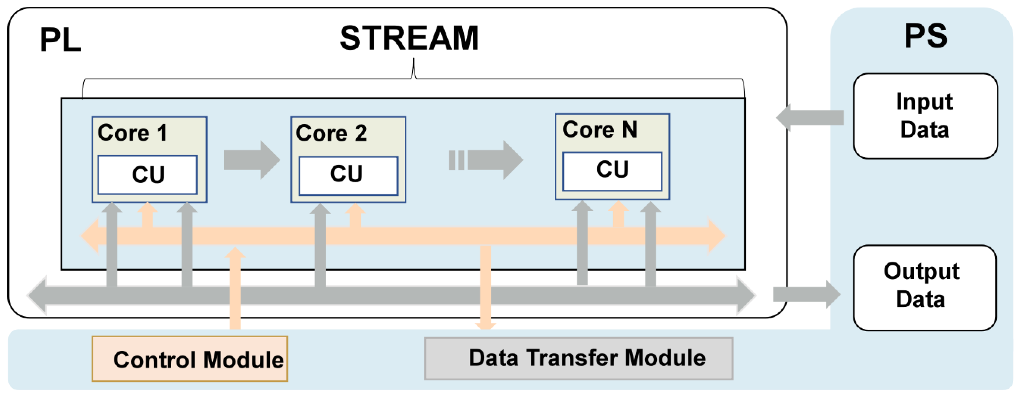
In order to improve the efficiency of data prediction, we deployed CBPNN as an edge intelligent node on the FPGA development platform. The key to implementing a neural network FPGA is to establish the architecture, including data transmission, temporary storage, and result reading. The deployment of neural networks requires not only matrix operations of weights and activation values as well as the output of activation functions but also effective optimization of the FPGA architecture design to improve real-time performance in practical applications. Therefore, the core of the design includes the design of a neural network accelerator and hardware architecture, as shown in Figure 4.

Figure 4.
The system architecture diagram.
4. Specific Algorithm Design
4.1. Design of Parameter Prediction Algorithms
CBPNN is deployed as a prediction algorithm for edge computing nodes. The network volume must be very small, and the output must be prevented from overfitting. Therefore, an architecture was designed with four small single hidden layer BPNN cascades, some of which had external inputs. The input of the first layer neural network is fitted with the position parameters of BPM1 and the current intensity values (M1x, M1y, M2x, and M2y) of the two magnets M1 and M2. The second layer of the neural network obtains input variables from the output results of the first layer and the current intensity of the M3 magnet. This layer of the neural network predicts the position of BPM3 through a single hidden layer network composed of eight neurons. The third layer of the cascaded network consists of the fitting results of BPM3 position data and the current intensity of the two magnets M4 and M5 as input variables and outputs BPM4 position parameters after a single hidden layer network of 12 neurons. The input of the last layer comes from the position data of BPM4 and the current intensity of the M6 magnet, and the output is the position parameter of BPM5. These known quantities were used as inputs in the experiment to predict the position coordinates of subsequent BPM. The output data can be mapped to the relationship with the automatic beam correction system. The design of the cascaded BPNN network structure is shown in Figure 5.
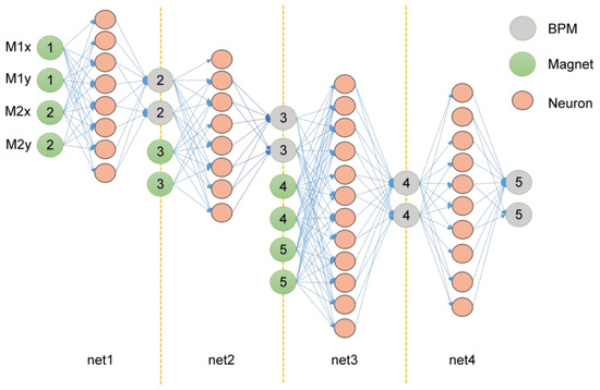
Figure 5.
CBPNN design structure.
Each layer in the designed cascaded neural network is composed of Leaky ReLU as the activation function. The advantage of using LeakyReLU is that it can also calculate the gradient for parts smaller than 0 in backpropagation, which solves the problem of gradient vanishing. The commonly used LeakyReLU activation function can be expressed as
Leaky helps to expand the range of the ReLU function; α is the adjustment factor of LeakyReLU, and the value of α is usually about 0.01. ReLU and LeakyReLU functions converge faster in training and have smaller computational complexity, so ReLU and LeakyReLU are easier to implement in edge node deployment. In HLS, ReLU function optimization can be achieved.
The experimental dataset was based on the simulation data generated by the TraceWin beam dynamics software TracePro 7.3.4, which was statistically processed for training and validation. The deterministic and non-deterministic factors in the experimental data were the grid of the MEBT and the strength of the corrected magnets, respectively, where the unmeasured factor was the error between the real and simulated particle accelerators.
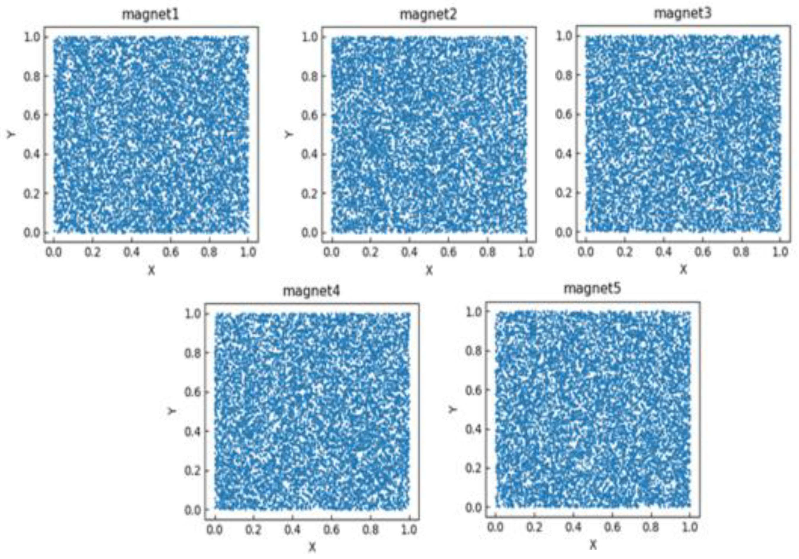
The scatter plot distribution of the training dataset is shown in Figure 6 and Figure 7, where the horizontal and vertical coordinates of each subgraph in Figure 6 represent the axis of its BPM data. From the figure, it can be seen that in the region where the point distribution r < 3 in BPM2 is affected by the neural network, the scatter distribution radius in BPM3 becomes smaller, with most particles distributed in the region where r < 2.5. Particles in BPM4 are more densely distributed, and most particles are distributed in the region where r < 2. Particles in BPM5 are more densely distributed in the region where r < 1.8. This indicates that CBPNN played a significant role in achieving successful particle focusing. In Figure 7, the X and Y axes represent the magnetic current intensity in two directions.
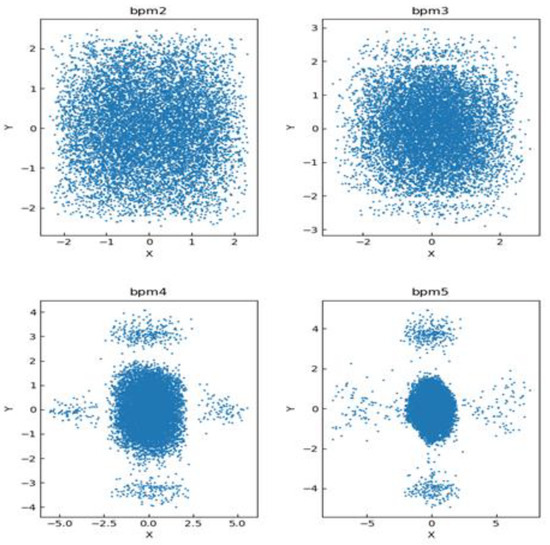
Figure 6.
Scatter plot of BPM training data.
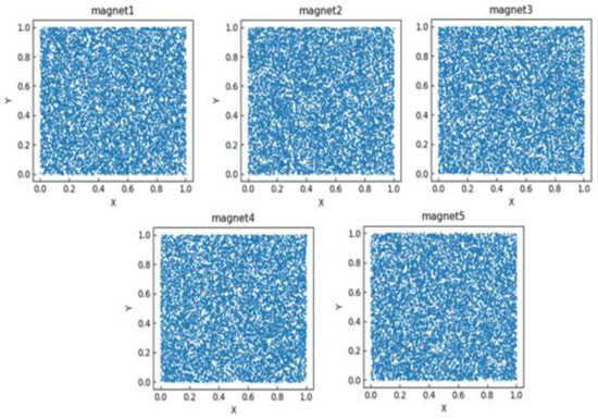
Figure 7.
Scatter plot of magnet strength parameter data for the magnet.
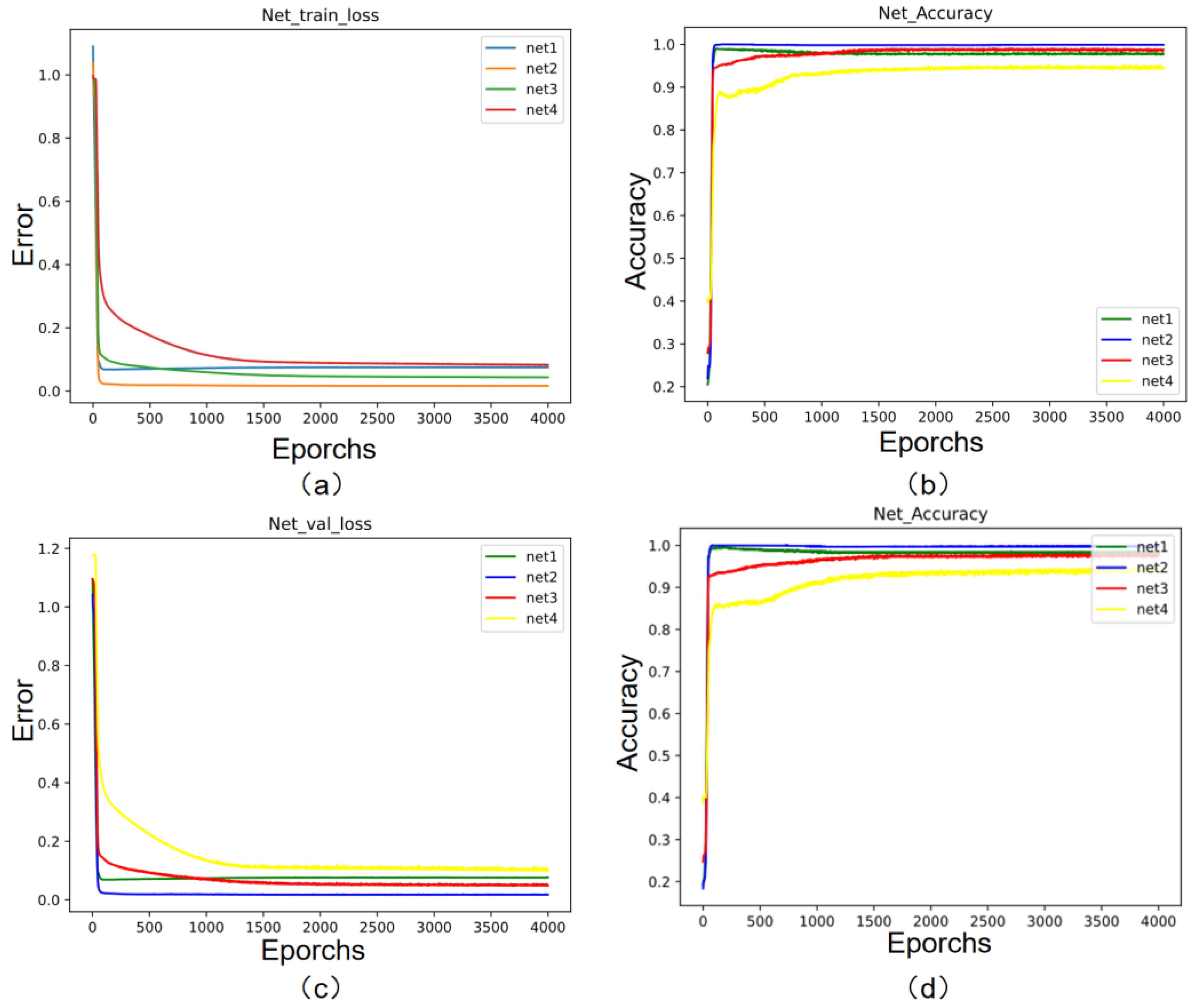
The training was based on the Pytorch platform, and 7000 rounds of training were carried out using randomly assigned 5000 sets of training data with the BatchSize set to 64. The testing and validation sets were tested, and the accuracy of the validation set was around 94.7%. The loss values of the neural network training and testing are shown in Figure 8. As can be seen, its four cascade network losses converge around the X-axis.
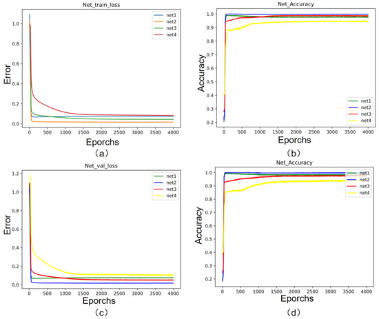
Figure 8.
Cascaded BPNN training and test loss values. (a) Training errors; (b); training accuracy; (c) verification errors; (d) verification accuracy.
4.2. FPGA-Based Parallel Acceleration Algorithm Design and Implementation
4.2.1. Hardware System Architecture Design
A neural network accelerator is deployed to the PL side of the ZYNQ platform, at which point its neural network forward reasoning acceleration has been completed. However, the hardware and software of the entire system need to be developed collaboratively in order to control the data flow; hardware acceleration alone can only accelerate its neural network data process. If the data flow transmission within the system is slow, then the deep learning acceleration effect is no longer good but also will not achieve good results in the overall system latency [19].
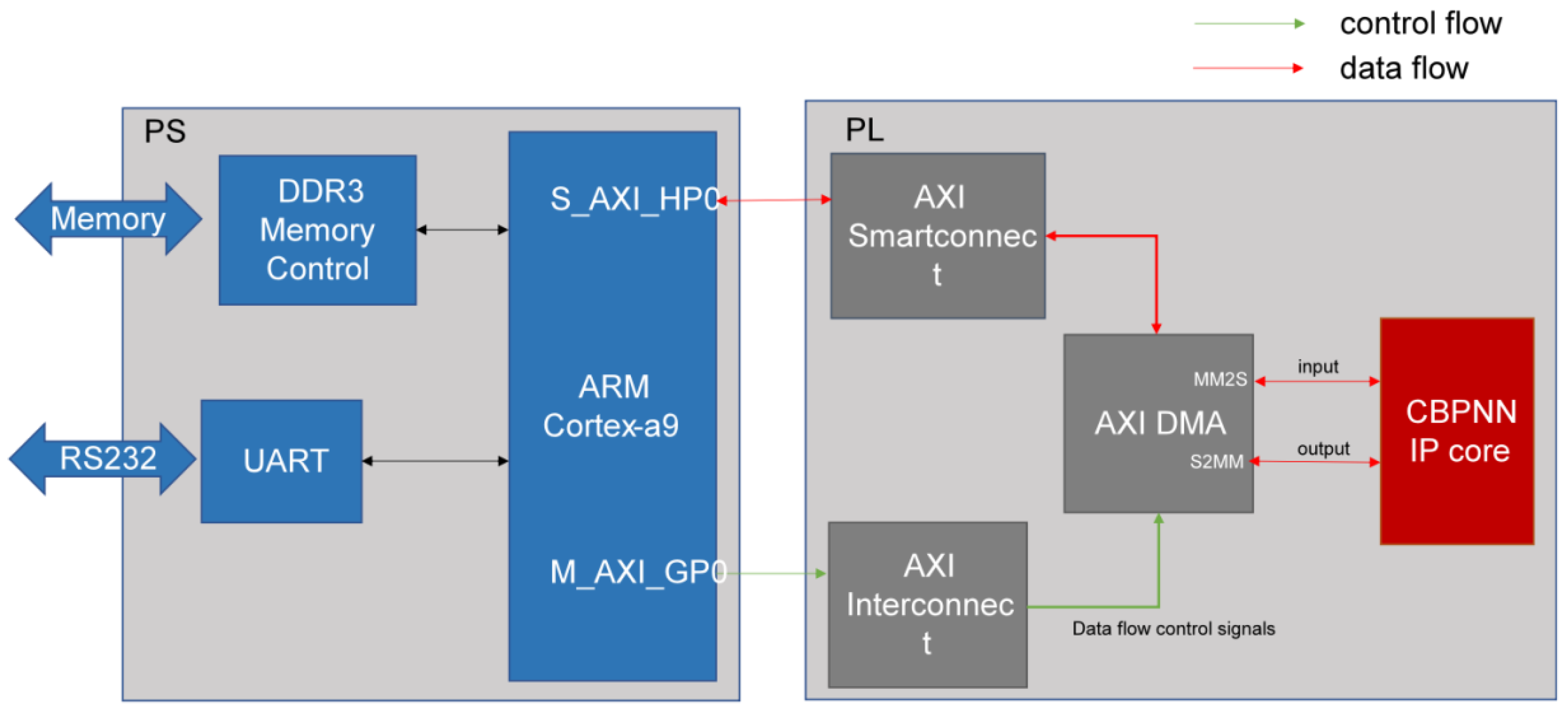
This paper presents an FPGA-based data transfer design for a neural network accelerator that utilizes efficient data interaction capabilities between PS (processing system) and PL (programmable logic) on the ZYNQ SOC platform. The neural network accelerator is a customized IP (intellectual property) core that accelerates the forward reasoning computation of the neural network. DMA is the mounting device on the PS side, which can realize efficient control of data transmission and greatly reduce the system transmission delay. The PS side schedules the data flow using AXI SmartConnect and the control flow using AXI interconnections. The MM2S and S2MM interfaces of the DMA receive the data and send the processed data, respectively, which completes the cycle of the data flow and the control flow, forming a closed loop. Figure 9 shows the block diagram of this hardware system design.

Figure 9.
Hardware system block diagram.
4.2.2. Sparse Training Algorithm
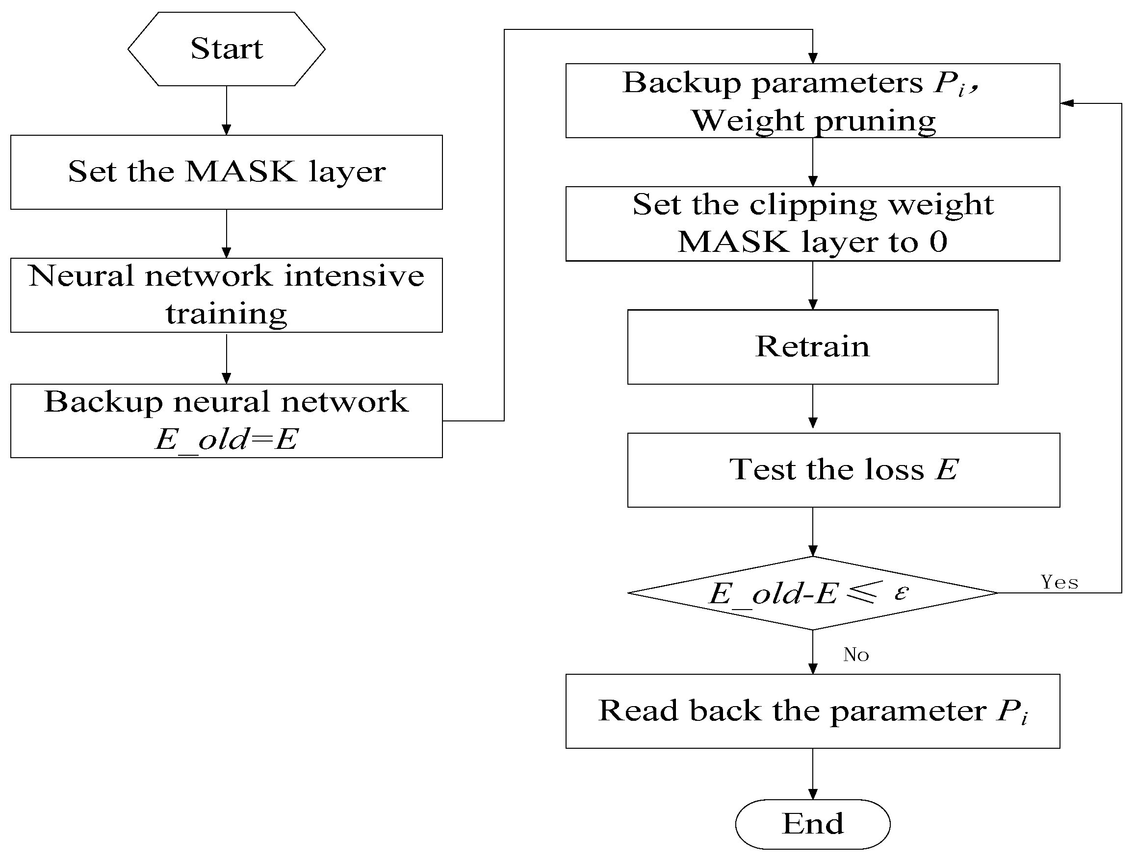
With the continuous improvement of deep neural network technology and the optimization of hardware platform performance, deep learning has superior performance in different applications. The sparse training algorithm improves the accuracy of neural networks and reduces the storage space of weights. By carrying out dense training, followed by sparse training, and then re-training, deep neural networks have made significant improvements in many fields. Deep neural networks have made significant improvements in many areas. Such a model has a very strong fitting ability and can effectively fit the nonlinear relationship between the input features and the output. However, they can introduce noise into the data itself, leading to problems such as overfitting and high variance [20]. The neural network sparsification retraining algorithm we used refers to the DSD algorithm. In the DSD algorithm, pruning can reduce storage space and sometimes improve accuracy by reducing weight connections [21].
We utilized the sparse training method to prune the neural network with the aim of enhancing its accuracy. This approach not only decreases the number of weights in the neural network, saving storage space on the deployed device, but also enhances the network by retraining through sparsifying the weight distribution. The initial model was first trained with a traditional dense model, followed by clipping weights to induce sparsity, and then retraining. The flowchart of sparse training is depicted in Figure 10. A key component of this algorithm involves adding a mask layer to the linear layer of the neural network to align with the neural network weight branches. Subsequently, during the pruning process, branches with weights closer to 0 are trimmed based on a predefined pruning threshold. This is because the nearer the weights of the neural network branches are to 0, the lesser their proportional contribution in the matrix cumulative multiplication of the forward inference. In the final retraining stage, the pruned branches are locked to prevent them from participating in the retraining process, while the remaining weights are re-adjusted.

Figure 10.
Flowchart of sparse training algorithm implementation.
The current design of the neural network deployment resources is compact, allowing deployment without extensive compression of the neural network size in ZYNQ. The primary objective of implementing the algorithm here is to enhance prediction accuracy while reducing the neural network weight resources. During training, the final model produced by sparse training maintains the same backbone as the original training model, and sparse training does not introduce additional waste of inference resources.
4.2.3. Fixed-Point Quantization Algorithm
Quantization refers to the representation of 32-bit floating-point parameters with lower bit widths, reducing inference time and parameter storage space. The robustness of the neural network enables quantization to maintain accuracy after processing the parameters. The floating-point multiply–accumulate operation of the matrix can be replaced by the multiply–add and shift operations of the quantized data, which significantly reduces the consumption of DSP (digital signal processing) resources because of floating-point operations. Quantization is mainly divided into post-training quantization and quantization-aware training. Post-training quantization does not require retraining or labeling of data and is a lightweight quantization method. In most cases, post-training quantization is sufficient to achieve 8-bit quantization with near-float precision. Quantization-aware training requires fine-tuning and access to labeled training data, enabling low-bit quantization with lower precision loss. The fixed-point quantization method is more suitable for deployment because the design is deployed on an FPGA platform, which has more efficient fixed-point acceleration.
Fixed-point quantization represents numbers as a combination of integers and decimals. The first step is to determine the range and precision of the fixed-point representation, which is determined by the bit width. The precision is determined by the decimal point position. By selecting the appropriate bit width and decimal point position, the resources required can be minimized while satisfying both accuracy and range. The required data type and data width are specified based on the bit width and decimal point position of the selected number of digits. Finally, according to the bit width and decimal place of the selected point number, the floating-point number is converted to the corresponding fixed-point number representation.
Fixed-point quantization algorithms are widely used in fields such as digital signal processing and machine learning to convert high-precision data to low-precision data to solve the problem of lack of precision in high-precision calculations when performing high-speed calculations in embedded systems. Fixed-point quantization algorithms convert floating-point numbers to fixed-point numbers through different rounding functions. Downward rounding causes precision loss, while upward rounding may cause overflow. Therefore, fixed-point quantization algorithms need to choose the appropriate rounding method and number of quantization bits according to the application scenario and requirements.
4.2.4. Design of Cascade Neural Network IP Cores and Acceleration Algorithms
According to the design requirements, HLS tools can quickly design and verify the neural network IP core design. By using C/C++ functionality with RTL, FPGA components can be implemented in a software environment, enabling the development of functional verification for this module within the software environment. This approach seamlessly combines hardware simulation environments and utilizes software-centric tools for reporting and optimizing the design. Traditional FPGA design tools can then be used to quickly generate IP.
The design IP core interface uses the s_axilite interface to pass data of type ap_axis, representing an axis with a 32-bit width and four channels. Each of these channels has 5 bits for valid data and another 5 bits for channel validity or other control information. This representation is often used to describe data flow or data paths in hardware designs. Matrix operations are performed by converting the received data formatted as ap_axis to fixed-point numbers.
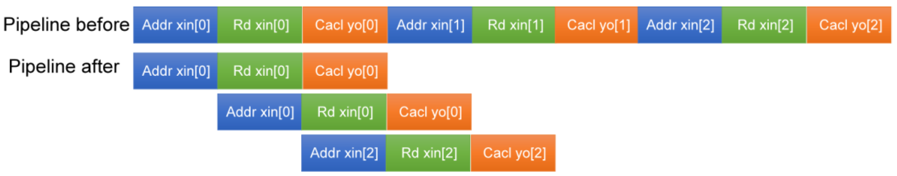
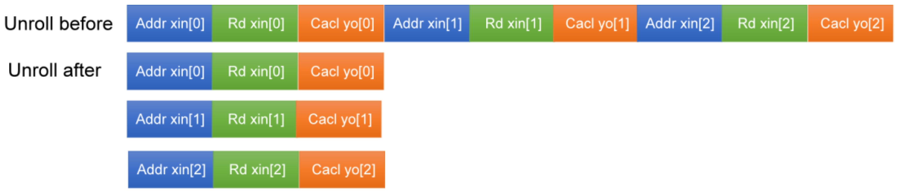
CBPNN, as a fully connected neural network, computes the weighted sum of matrix multiplication and cumulative bias, so the optimization of the matrix multiplication is the core of the design. To meet the requirement of interacting with multiple intelligences, it is essential to enable each sub-network of the cascade neural network to interact with separate data streams. State machine algorithms are introduced to facilitate this. The four sub-networks are designated as four states, satisfying both the overall output of the CBPNN and the individual sub-networks interaction with intelligence. In HLS, pipelining allows different computational stages in an algorithm to be processed in parallel, and each stage can independently complete specific operations within their respective clock cycles. The forward propagation of a neural network can be divided into multiple stages by pipelining, such as weighted input computation, activation function processing, summarization, etc. The results can be passed to the next stage immediately after each stage is processed without waiting for the entire network processing to be completed. The pipelining process is schematically shown in Figure 11. Loop unrolling is typically used to process neurons and hierarchies in a network. A typical loop may traverse all neurons of a neural network to compute the output. By using the loop unrolling algorithm, the iterative operation of processing each neuron in the loop can be changed to a parallel operation, i.e., the computation of multiple neurons can be processed at the same time, which greatly enhances the real-time processing of the algorithm. The loop unrolling process is schematically shown in Figure 12.

Figure 11.
The pipelining process.
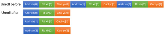
Figure 12.
The unroll process.
In this study, we used the optimization method of pipelining and loop expansion. The pseudo-code of the matrix multiplication algorithm is shown in Algorithm 1, which shows that there are mainly five loops, two matrix multiplication calculations, and cumulative bias. Matrix multiplication is supposed to be the superposition of the elements of each row of A by the corresponding elements of each column of B. The matrix multiplication algorithm is a simple technique that helps simplify complex calculations and solve systems of linear equations. The innermost loop of the matrix multiplication logic is the product of the elements of the i row of A and the elements of the j column of B. The outer loop is the product of the elements of the j column of B and the elements of the j column of A. Its outer layer is a column traversal of matrix B, which allows it to compute all the elements of its i row, and the outermost loop is a traversal of the rows. Matrix–vector multiplication is defined as
| Algorithm 1. Deep learning forward propagation (three-layer weight matrix connected multiplication phase) | |
| Input: | |
| Output: | |
| 1. | for i = 0 to K − 1 do |
| 2. | #pragma unroll // Instruction unroll |
| 3. | for j = 0 to N − 1 do |
| 4. | |
| 5. | end for |
| 6. | end for |
| 7. | LeakyRelu(output1); Activation function to organize data features |
| 8. | for i = 0 to K − 1 do |
| 9. | #pragma pipeline // Instruction pipelining |
| 10. | for j = 0 to N − 1 do |
| 11. | |
| 12. | end for |
| 13. | end for |
Matrix operations are a major consumer of computational resources. For the designed CBPNN, the main acceleration focus is on the forward propagation part; the forward propagation is composed of cumulative multiplication, and the input and output data are the same as the designed neural network. To improve the loop parallelism performance, we used loop unrolling and pipelining techniques. Loop unrolling makes multiple copies of the loop body and performs a set of iterations simultaneously on hardware. Its parameter specifies the number of iterations to be executed in parallel on hardware at a time. Loop unrolling not only addresses the issue of underutilization but also aids in optimizing the data path and on-chip memory design. FPGA pipelining involves decomposing a complex computational task into multiple sub-tasks and processing them in a pipeline. FPGA deployment of neural networks for pipelining was designed and optimized using reconfigurable resources on the FPGA, employing the DSP for matrix operations and LUTs for logic operations and lookup table operations. The overall hardware accelerator internal architecture is shown in Figure 13.
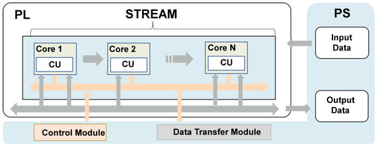
Figure 13.
Hardware accelerator internal architecture.
5. Tests and Discussions
We developed and trained a CBPNN with a BPM5 prediction error of only 0.135 mm using PyTorch on the server and deployed it in an edge acceleration node based on an FPGA development board. We then tested the algorithm performance during the model deployment process, including the pruning algorithm, quantization effectiveness, hardware performance indicators, hardware acceleration performance, and feasibility of the hardware system architecture.
5.1. Hardware and Software Experimental Environment
In this study, the experimental development board used was ZYBO-Z7, with a main frequency of 120 MHz. The CPU control group used was a 12th Gen Intel(R) Core(TM) i5-12490F 3.00 GHz processor, with a main frequency of 3 GHz; the number of processors was 6 cores and 12 threads, and it had the Windows operating system. The GPU control group used an NVIDIA GeForce GTX 1660 SUPER chip with 1408 CUDA cores, a core frequency of 1530 MHz, 6 GB of video memory, and the Windows operating system. Experiments were conducted on the ZYBO-Z7 development board for this design, and the resource utilization of the hardware accelerator is shown in Table 1.

Table 1.
Resource utilization of hardware accelerators.
As can be seen from Table 2, the resource utilization of the accelerator BRAM was 0. This was because the model parameters of the current cascade neural network were not large, and the parameters were optimized by implementing them in the LUT. The future deployment of large-scale neural networks will require deploying the parameters into the BRAM.
Table 2.
Comparison of resources before and after hardware accelerator optimization.
5.2. Hardware Accelerator Acceleration Effect Test
In order to test the performance of the hardware acceleration algorithm, we first tested the resource occupancy and computation required for the clock cycles of the CBPNN deployed in FPGAs under non-optimized conditions. Then, matrix computation acceleration, loop pipeline, and loop deconvolution were used for operational optimization, and hardware resource utilization and clock cycles were tested again. The test results are shown in Table 2. We found that after applying optimization algorithms, the utilization rate of DSP48E increased by 37%, indicating a significant improvement in the parallel computing efficiency of the algorithm. At the same time, the occupancy rate of LUT increased by 31%, and the clock cycle was reduced by 1152. This indicates that the algorithm significantly improved the computation speed by increasing the utilization rate of LUT and DSP38E. The hardware accelerator accelerated the algorithm by about 2.91 times, and the simulation forward inference time of the hardware accelerator was 5.52 μs.
5.3. Sparse Training Algorithm Performance Test
The purpose of sparse training algorithms is to identify and remove redundant parameters from neural network parameters, making the network weights sparse and thereby improving computational efficiency. The specific approach is to use sparse training algorithms to reset some weights of the neural network to zero and retrain it after training a well-performing neural network, ensuring that the network’s prediction accuracy does not decrease significantly. By repeatedly experimenting in this way, the optimal pruning ratio and sparsity parameters of the neural network can be obtained.
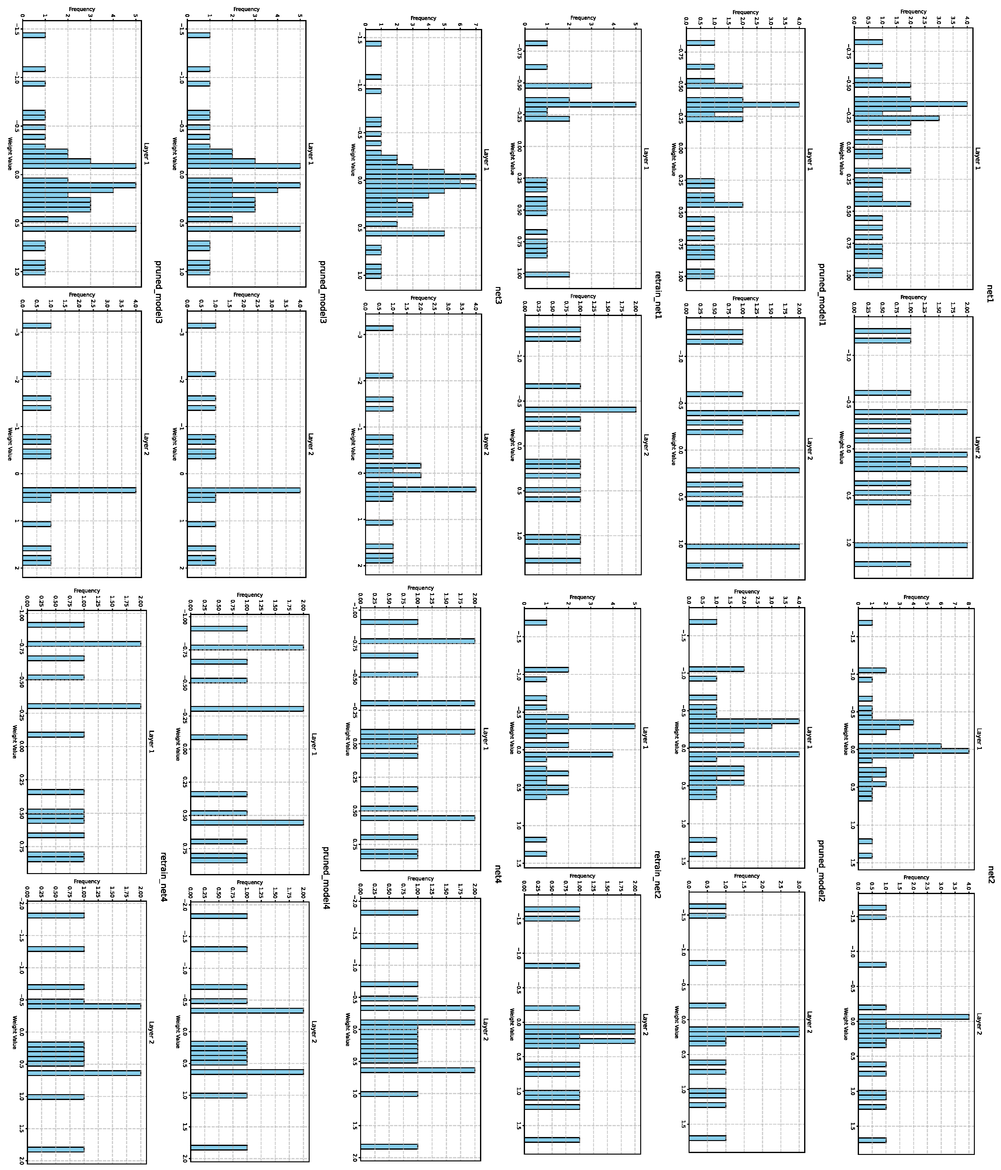
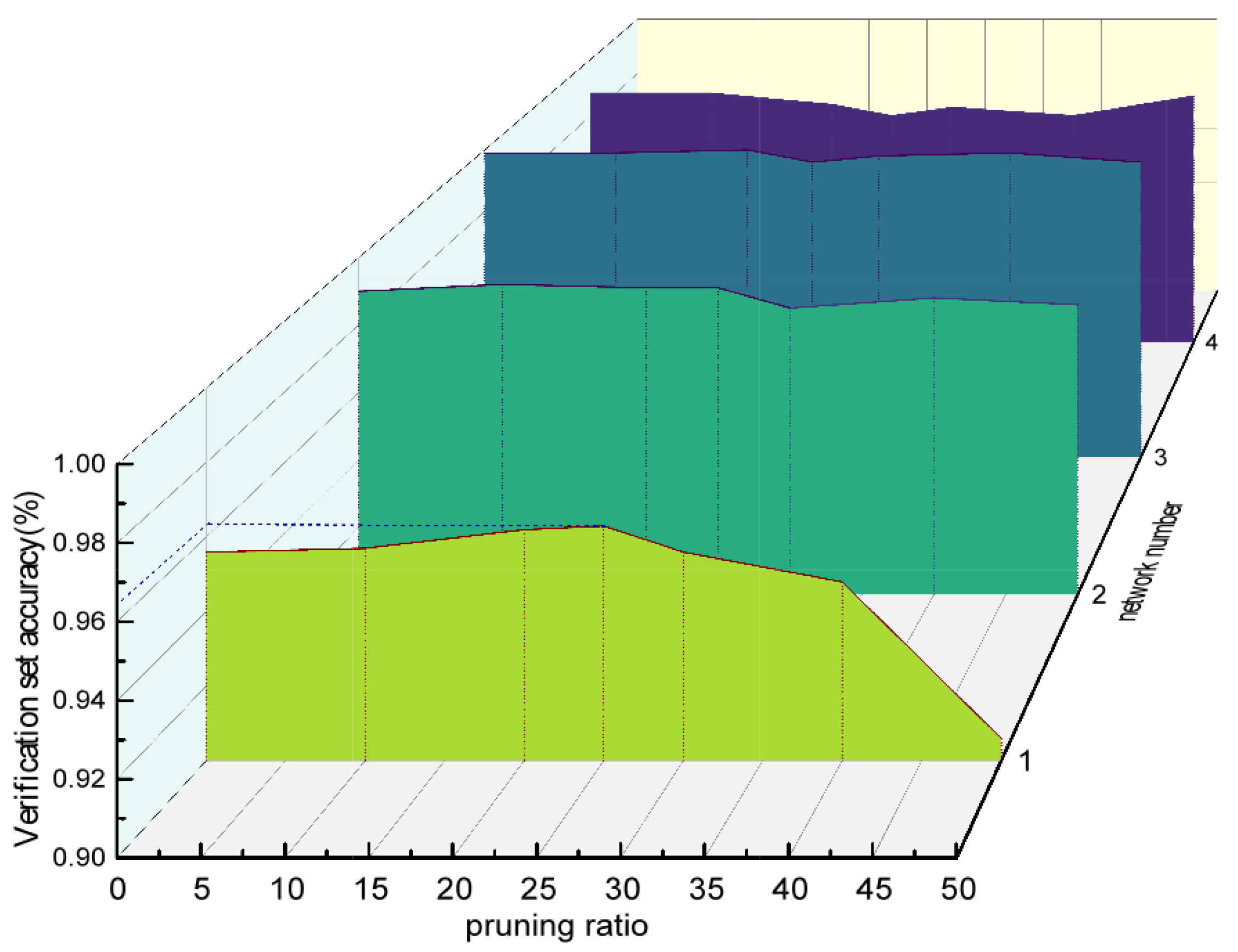
In the experiment, we first carried out extensive training and obtained the neural network with the best performance. Then, the parameters were trimmed by 10%, 20%, 30%, 40%, and 50% to test the accuracy of the neural network’s predictions. The experiment found that the accuracy of the neural network changed the most when the parameter pruning ratio was between 20% and 30%. Further experiments showed that when a parameter pruning ratio of 25% was selected, the prediction accuracy of the neural network still improved to some extent. Therefore, 25% was chosen as the final pruning rate for this experiment. Finally, through sparse training algorithms, the accuracy of the designed cascaded CBPNN was improved to 96.3%, an increase of 1.5%. As shown in Figure 14, the weights of each of the three processes after sparsity changed; their corresponding network numbers are labeled on the graphs. Each subgraph represents the weight of the current layer in the current sub-network. The second row of subgraphs corresponds to the weight changes after sparsity, and the third row corresponds to their weight distribution after training and sorting sparsity. Through experiments, it was found that after initial sparsity, their weights decreased, and the absolute values of the weight branches approached 0. This is because in the matrix multiplication operation of forward propagation, the closer the weight branches are to 0, the smaller the impact on the results. After training, the trimmed branches did not recover but were adjusted for quick fitting, ultimately restoring accuracy and changing the weight distribution. Figure 15 shows the effectiveness of the algorithm in improving accuracy at different pruning rates.
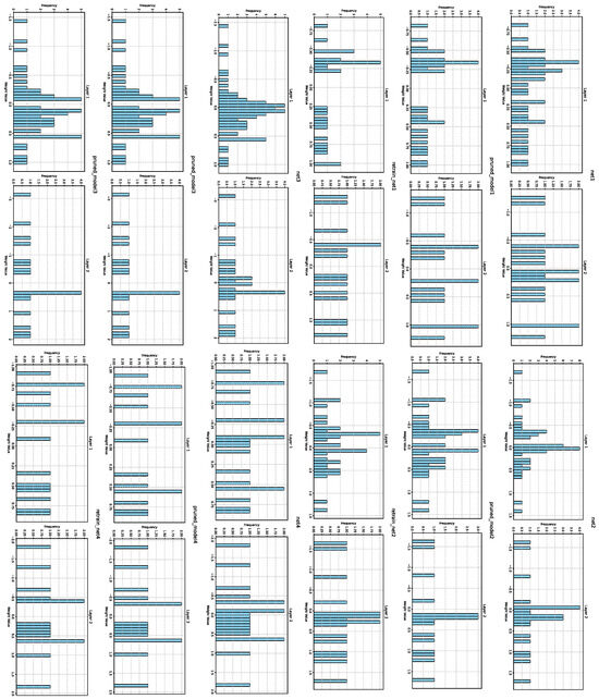
Figure 14.
Comparison of the three-stage weight distribution of the retraining algorithm after sparsification.

Figure 15.
Sparsification weight test results.
5.4. Quantitative Performance Testing
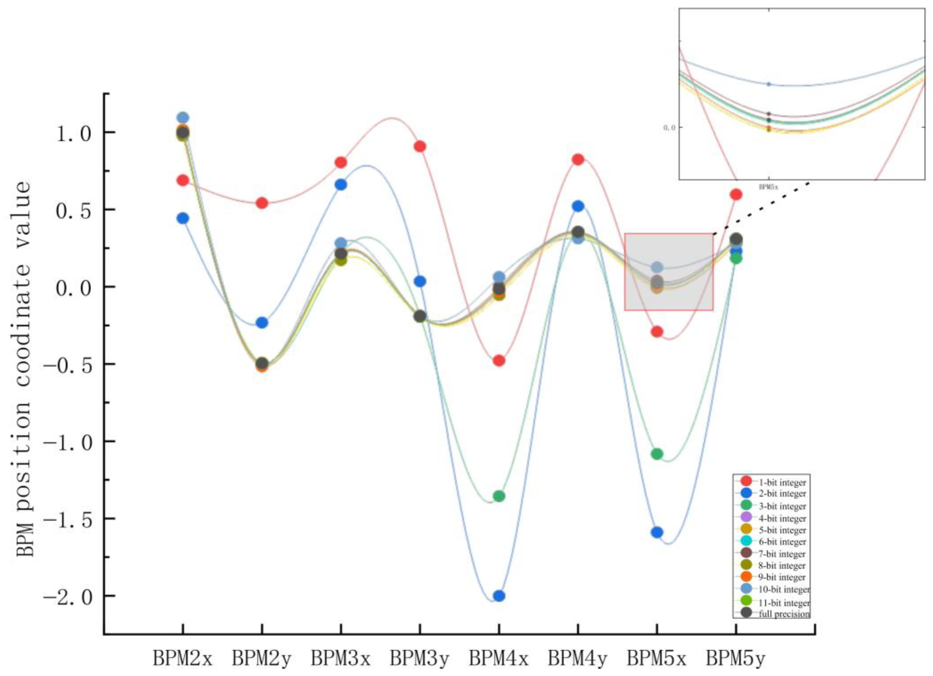
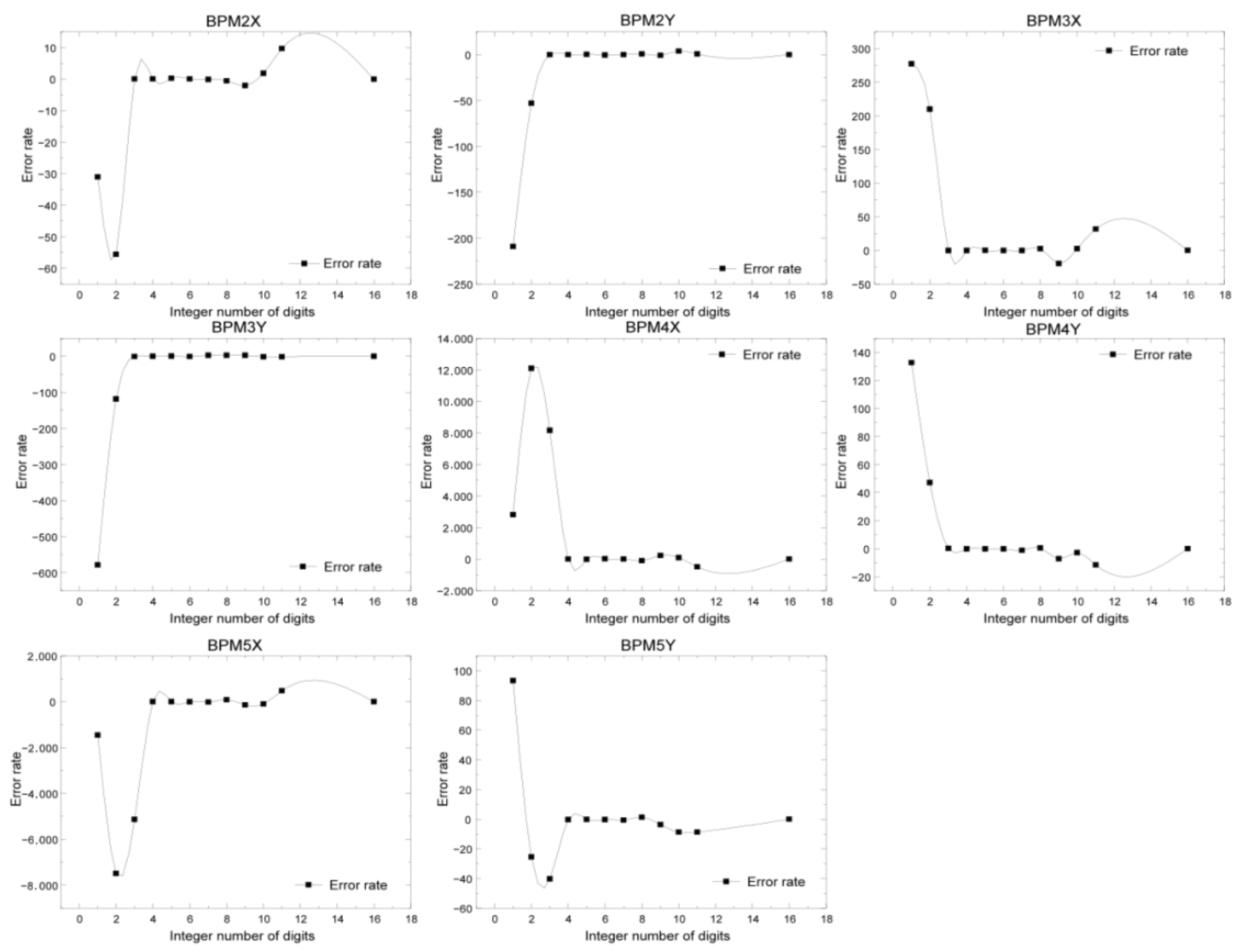
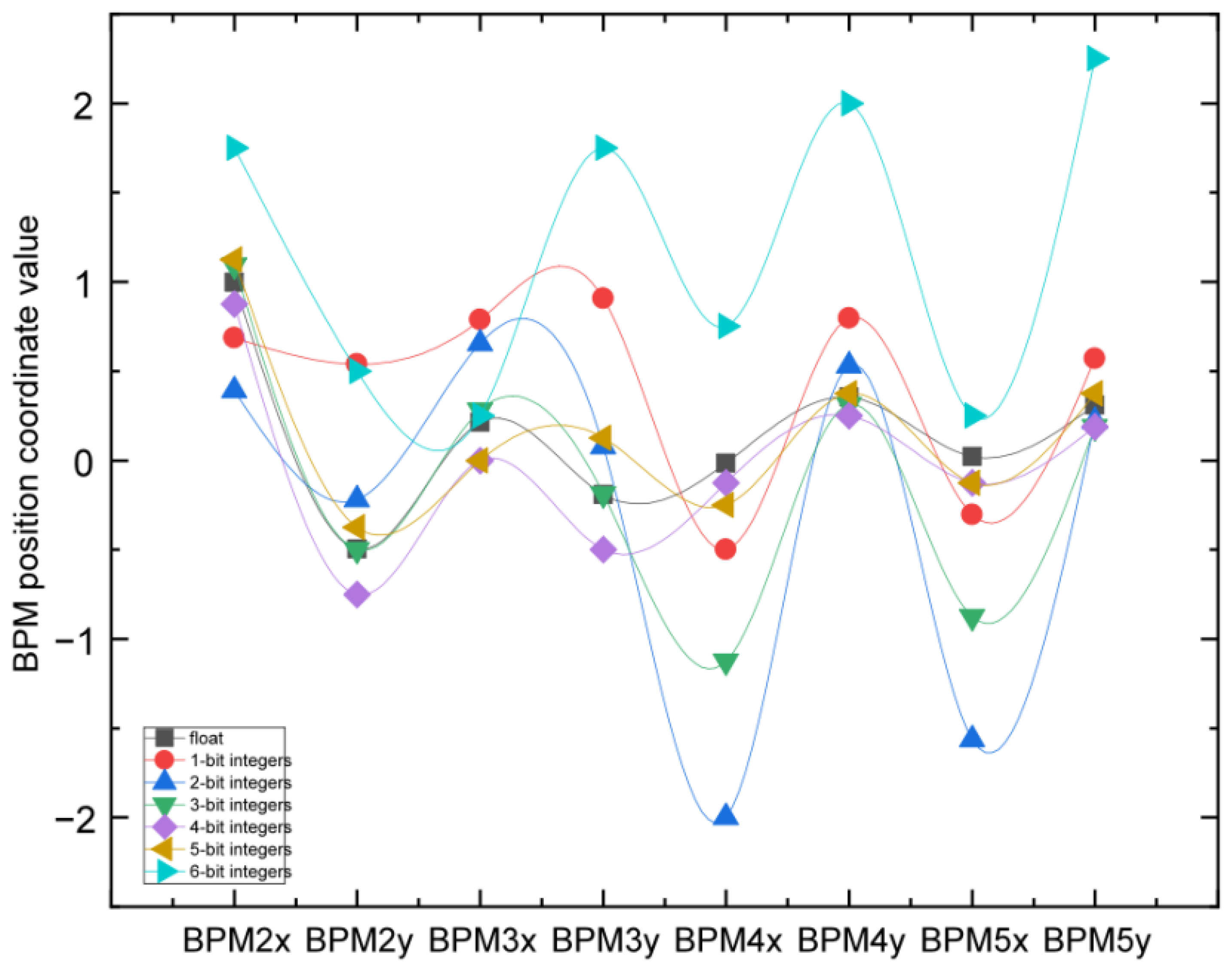
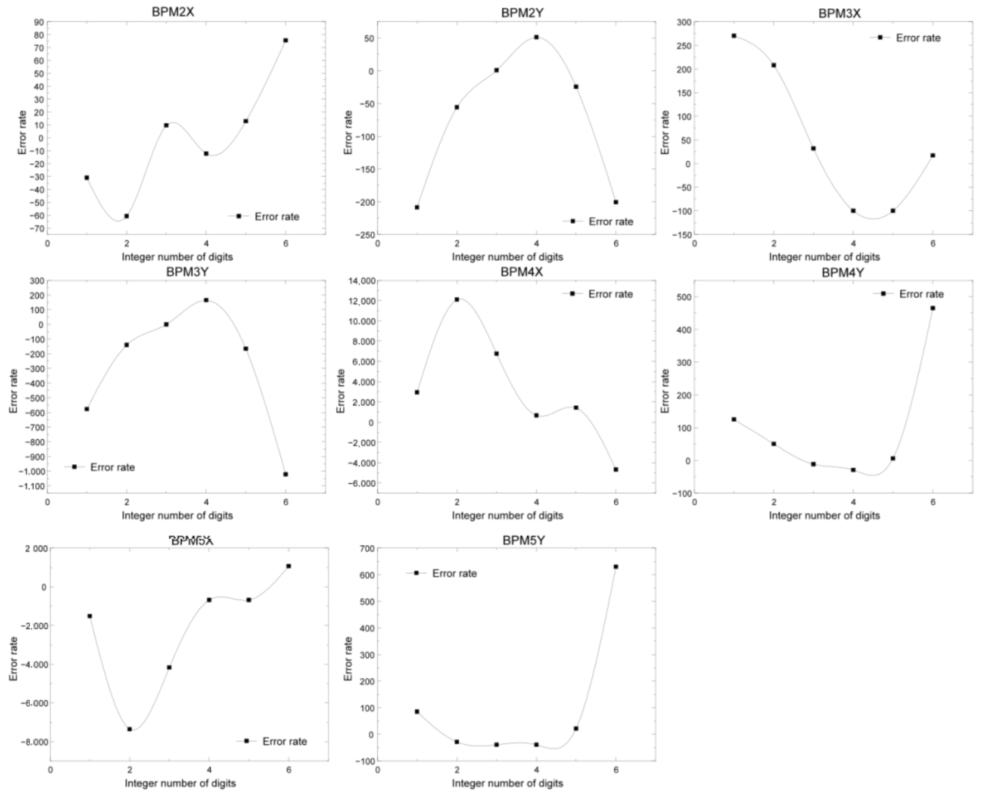
Before parameter quantization, it is necessary to convert the parameters of the neural network from floating-point numbers to fixed-point numbers and then round them after determining the quantization number in order to test the errors of different fixed-point quantization algorithms. We quantized the weight parameters of the neural network into 8, 16, and 32 bits and conducted experiments on 8-bit, 16-bit, and 32-bit quantization of integer bits to test their impact on the prediction accuracy of the neural network. The experimental results of fixed-point quantization algorithms with different integer bits are shown in Figure 16 and Figure 17. The points in Figure 16 represent the coordinate parameters of the corresponding BPM positions. From the results, it can be seen that the coordinate parameters of the 16-bit fixed-point quantization algorithm with four integer digits were almost the same as those of the 32-bit fixed-point position parameter, with the smallest accuracy loss, while the accuracy loss of 8-bit quantization was significant. Each subgraph in Figure 17 represents the error rate predicted by the neural network when the number of fixed-point digits was 16 and the number of integer digits was was different. From the graph, it can be seen that when the number of integer digits was 8 and the number of fixed-point digits was 16, the error rate of the neural network was the lowest.
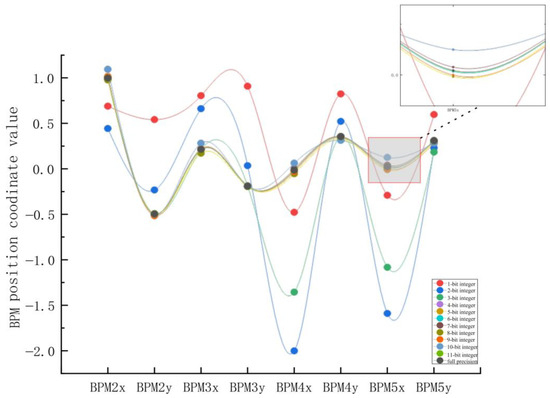
Figure 16.
Experimental results of the 16-bit fixed-point quantization algorithm with different integer digits.
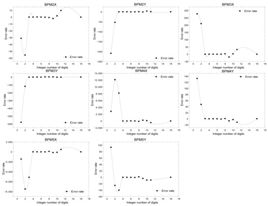
Figure 17.
Comparison of the error rate of the 16-bit fixed-point operation with different integer bits for different coordinates of BPM.
Then, we conducted an 8-bit fixed-point accuracy test, and the test results are shown in Figure 18 and Figure 19. The comparison between 8-bit fixed-point quantization and floating-point values showed significant errors. In Figure 18, each subgraph has errors of different integer bit sizes, with a maximum precision loss of over 50%. The 8-bit fixed-point quantization error was relatively large because the range of input values had exceeded the range of 8-bit fixed-point values, resulting in severe error offset. Therefore, this design adopted 16-bit fixed-point quantization, where both integers and decimals were 8 bits.
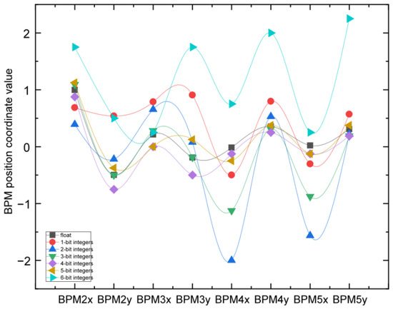
Figure 18.
Comparison of the prediction results of 8-bit fixed-point quantization with different integer bits.
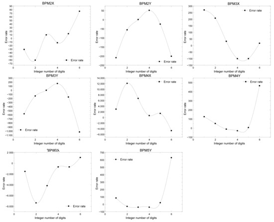
Figure 19.
Comparison of the error rate of the 8-bit fixed-point operation with different integer bits for different coordinates of BPM.
5.5. Hardware Performance Evaluation
In this experiment, mainstream hardware acceleration devices were selected as the control group to test the performance indicators of the acceleration platform, including GPU and CPU devices. The test data were generated from 3000 sets of data using TraceWin beam dynamics software that had undergone statistical processing. For GPU and CPU platforms, a configuration file tool was used for forward inference analysis to obtain their forward inference latency under current power consumption conditions. The processing time, network inference time, and computational complexity of each set of data on different computing platforms were tested, as was the platform power consumption. We then randomly selected 10 sets of data from the validation set and input them into the ZYBO-Z7, GPU, and CPU computing platforms. The power consumption test of the FPGA development board is shown in Table 3. From Table 3, it can be seen that the average inference time of the cascaded neural network of this hardware accelerator was about 28 μs, and the computing speed was 12.66 times that of the GPU and 35.66 times that of the CPU, indicating that the edge intelligent node designed in this study achieved significant acceleration on the FPGA.
Table 3.
Accelerated platform performance test comparison.
The computing power of the CBPNN network was 320 FLOP, so the effective computing power of this accelerator per second was 15.714 MOPS, and the energy efficiency ratio was 10.582 MOPS/W. The energy efficiency ratio of this accelerator was 410.16 times that of the GPU and 988.97 times that of the CPU. The actual power consumption of the FPGA was 1.572 W, which was much lower than the power consumption of the GPU and CPU devices. The experimental results show that the edge computing node designed in this work has the characteristics of good acceleration performance, low energy consumption, and a high energy efficiency ratio and improves the real-time performance of the algorithm.
From Table 3, it can be observed that in this experiment, the deployment speed of the GPU will be much slower than that of the FPGA platform, as this phenomenon needs to be discovered from the deployed neural network. From the structure diagram of the deployed cascaded neural network, it can be seen that three of the four BPNN input channels require external input, and multiple data inputs are needed to be called in the GPU. This data-calling process will greatly slow down the forward inference latency of the GPU.
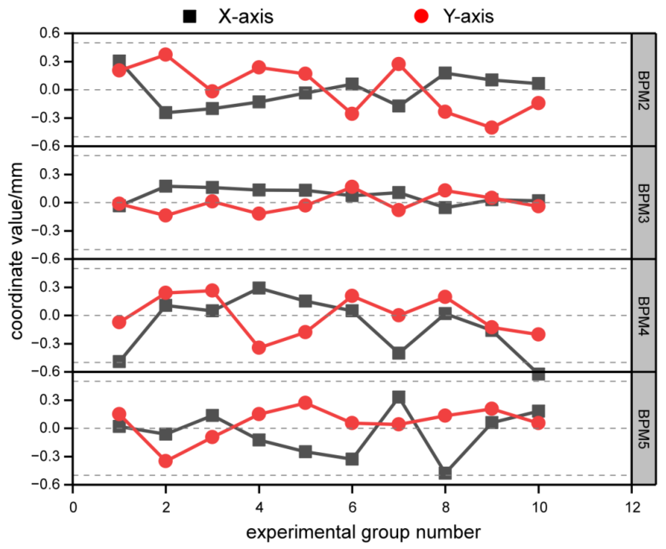
5.6. Accuracy Testing
Ten sets of data extracted from the validation dataset were input into an FPGA-based deep learning acceleration node for accuracy testing. Then, the obtained predicted data were compared with the original dataset to calculate the error between each set of predicted results and the actual results, as shown in Figure 20. In the figure, the four figures correspond to the X-axis and Y-axis errors of BPM2, BPM3, BPM4, and BPM5, respectively. The black box represents the X-axis data, while the red circle represents the values on the Y-axis. After experimental testing, it was found that the X-axis and Y-axis errors of the 10 test groups were all less than 0.5 mm, meeting the accuracy requirements for predicting actual beam current control.

Figure 20.
BPM prediction error. Due to the specificity of the BPM prediction error, the general requirement in practice is that the error is less than 0.5 mm, which means it is accurate, and it can be seen that the error of each BPM coordinate data meets this requirement.
6. Conclusions and Future Work
The study aimed to enhance the mapping speed of BPM location data parameters by employing BPM location data prediction as a system architecture design validation scheme, aligning with reinforcement learning for automatic beam correction. We propose a system architecture for deploying edge intelligence acceleration nodes using the ZYNQ development board, emphasizing low latency and energy efficiency. In our experiments, FPGA-accelerated forward inference outperformed GPU and CPU platforms, exhibiting significantly higher energy efficiency, which is particularly suitable for large-scale deployment. According to the experimental results, the proposed hardware accelerator achieved an average prediction accuracy of 96.3% with an average inference latency of 5.52 μs in BPM location prediction applications. As an edge acceleration platform for neural networks, the FPGA-accelerated neural networks delivered exceptional acceleration, with delays reaching the microsecond level, validating the system’s low latency and high energy efficiency ratio and fulfilling the practical requirements of beam orbit parameter prediction.
However, this work was conducted using virtual particle accelerator data. For real particle accelerator beam track data prediction schemes, additional considerations of factors influencing beam correction are necessary. Future work will entail incorporating more influential factors from real particle accelerators into deep learning training, improving neural network model deployment methods, and optimizing data transfer architectures to fully integrate reinforcement learning into edge smart acceleration nodes for automated beam current correction. Our goal is to integrate reinforcement learning into an adaptive compensation beam current correction system and apply it in real particle accelerators.
Author Contributions
Writing—original draft, M.H.; Project administration, Y.G.; Formal analysis: G.Y.; Methodology, Writing—review & editing: X.Y.; Software: Z.C.; Resources: Y.C.; Conceptualization, Y.H. All authors have read and agreed to the published version of the manuscript.
Funding
This work was partially supported by the Youth Innovation Promotion Association CAS (Grant No. 2018452), the Large Research Infrastructures “China Initiative Accelerator Driven System” (Grant No. 2017-000052-75-01-000590), the Gansu Key R&D Projects under Grant No. 23YFGA0013, and the Gansu Sci. & Tech. Program under Grant No. 22JR11RA134.
Data Availability Statement
The original contributions presented in the study are included in the article, further inquiries can be directed to the corresponding author/s.
Conflicts of Interest
The authors declare no conflict of interest.
Abbreviations
The following abbreviations are used in this manuscript:
| CiADS | China Initiative for Accelerator Driven System |
| BPNN | backpropagation neural network |
| CBPNN | cascaded backpropagation neural network |
| CNN | convolutional neural networks |
| RL | reinforcement learning |
| FPGA | field programmable gate arrays |
| HLS | high-level synthesis |
| DSP | digital signal processing |
| LUT | lookup table |
| BPM | beam position monitor |
| RFQ | radio frequency quadrupole |
| MEBT | medium energy beam transport line |
| GPU | graphics processing unit |
| CPU | central processing unit |
| IMP | Institute of Modern Physics |
| CERN | European Organization for Nuclear Research |
References
- Yang, X.; Chen, Y.; Wang, J.; Zheng, H.; Liu, H.; Zhou, D.; He, Y.; Wang, Z.; Zhou, Q. Online beam orbit correction of MEBT in CiADS based on multi-agent reinforcement learning algorithm. Ann. Nucl. Energy 2022, 179, 109346. [Google Scholar] [CrossRef]
- Yang, X. Neural Network-Based Calibration Technique for C-ADS Injector II Beam Offset. Ph.D. Thesis, Lanzhou University, Lanzhou, China, 2019. [Google Scholar]
- Qin, Y.; Wang, Z.; Feng, C.; Liu, S.; Dou, W.; Chen, W.; Wang, W.; Xie, H.; He, Y. Longitudinal Beam Parameters Measurement by Beam Position Monitors. Nucl. Phys. Rev. 2021, 38, 30–37. [Google Scholar]
- Wang, F.; Song, M.; Edelen, A.; Huang, X. Machine learning for design optimization of storage ring nonlinear dynamics. arXiv 2019, arXiv:1910.14220. [Google Scholar]
- Leemann, S.C.; Liu, S.; Hexemer, A.; Marcus, M.A.; Melton, C.N.; Nishimura, H.; Sun, C. Demonstration of machine learning-based model-independent stabilization of source properties in synchrotron light sources. Phys. Rev. Lett. 2019, 123, 194801. [Google Scholar] [CrossRef] [PubMed]
- Chen, X.; Jia, Y.; Qi, X.; Wang, Z.; He, Y. Orbit correction based on improved reinforcement learning algorithm. Phys. Rev. Accel. Beams 2023, 26, 044601. [Google Scholar] [CrossRef]
- Cao, Z.; Yan, C.; Yang, X.; Guo, Y. Accelerator beam orbit prediction based on multi-stage cascaded BP neural networks. High Power Laser Part. Beams 2023, 35, 124002. [Google Scholar]
- Biookaghazadeh, S.; Ravi, P.K.; Zhao, M. Toward multi-fpga acceleration of the neural networks. ACM J. Emerg. Technol. Comput. Syst. (JETC) 2021, 17, 1–23. [Google Scholar] [CrossRef]
- Xia, J.; Enemali, G.; Zhang, R.; Fu, Y.; McCann, H.; Zhou, B. FPGA-accelerated distributed sensing system for real-time industrial laser absorption spectroscopy tomography at kilo-Hertz. IEEE Trans. Ind. Inform. 2023, 2, 2529–2539. [Google Scholar] [CrossRef]
- Luo, Y.; Cai, X.; Qi, J.; Guo, D.; Che, W. FPGA–accelerated CNN for real-time plant disease identification. Comput. Electron. Agric. 2023, 207, 107715. [Google Scholar] [CrossRef]
- Fujii, T.; Sato, S.; Nakahara, H.; Motomura, M. An FPGA realization of a deep convolutional neural network using a threshold neuron pruning. In Proceedings of the Applied Reconfigurable Computing: 13th International Symposium, ARC 2017, Delft, The Netherlands, 3–7 April 2017; Proceedings 13. Springer International Publishing: Berlin/Heidelberg, Germany, 2017; pp. 268–280. [Google Scholar]
- Nagel, M.; Fournarakis, M.; Amjad, R.A.; Bondarenko, Y.; Baalen, M.V.; Blankevoort, T. A white paper on neural network quantization. arXiv 2021, arXiv:2106.08295. [Google Scholar]
- Ayachi, R.; Said, Y.; Abdelali, A.B. Optimizing neural networks for efficient FPGA implementation: A survey. Arch. Comput. Methods Eng. 2021, 28, 4537–4547. [Google Scholar] [CrossRef]
- Wang, K.; Liu, Z.; Lin, Y.; Lin, J.; Han, S. Haq: Hardware-aware automated quantization with mixed precision. In Proceedings of the Proceedings of the IEEE/CVF Conference on Computer Vision and Pattern Recognition, Long Beach, CA, USA, 15–20 June 2019; pp. 8612–8620. [Google Scholar]
- Alam, S.A.; Gregg, D.; Gambardella, G.; Preusser, T.; Blott, M. On the RTL Implementation of FINN Matrix Vector Unit. ACM Trans. Embed. Comput. Syst. 2023, 22, 1–27. [Google Scholar] [CrossRef]
- Hirschauer, J.; Jindariani, S.; Tran, N.; Carloni, L.P.; Guglielmo, G.D.; Harris, P.; Krupa, J.; Rankin, D.; Valentin, M.B.; Hester, J.; et al. hls4ml: An open-source codesign workflow to empower scientific low-power machine learning devices. arXiv 2021, arXiv:2103.05579. [Google Scholar]
- Sharma, S.; Athaiya, A. Activation functions in neural networks. Towards Data Sci. 2017, 6, 310–316. [Google Scholar] [CrossRef]
- Apicella, A.; Donnarumma, F.; Isgrò, F.; Prevete, R. A survey on modern trainable activation functions. Neural Netw. 2021, 138, 14–32. [Google Scholar] [CrossRef]
- Han, S.; Pool, J.; Narang, S.; Mao, H.; Gong, E.; Tang, S.; Elsen, E.; Vajda, P.; Paluri, M.; Tran, J.; et al. Dsd: Dense-sparse-dense training for deep neural networks. arXiv 2016, arXiv:1607.04381. [Google Scholar]
- Lall, A.; Tallur, S. Deep reinforcement learning-based pairwise DNA sequence alignment method compatible with embedded edge devices. Sci. Rep. 2023, 13, 2773. [Google Scholar] [CrossRef] [PubMed]
- Nobari, M.; Jahanirad, H. FPGA-based implementation of deep neural network using stochastic computing. Appl. Soft Comput. 2023, 137, 110166. [Google Scholar] [CrossRef]


Disclaimer/Publisher’s Note: The statements, opinions and data contained in all publications are solely those of the individual author(s) and contributor(s) and not of MDPI and/or the editor(s). MDPI and/or the editor(s) disclaim responsibility for any injury to people or property resulting from any ideas, methods, instructions or products referred to in the content. |
© 2024 by the authors. Licensee MDPI, Basel, Switzerland. This article is an open access article distributed under the terms and conditions of the Creative Commons Attribution (CC BY) license (https://creativecommons.org/licenses/by/4.0/).