Comprehensive Analysis of Improved Hunter–Prey Algorithms in MPPT for Photovoltaic Systems Under Complex Localized Shading Conditions

Abstract

The Hunter–Prey Optimization (HPO) algorithm represents a novel population-based optimization approach renowned for its efficacy in addressing intricate problems and optimization challenges. Photovoltaic (PV) systems, characterized by multi-peaked shading conditions, often pose a challenge to conventional maximum power point tracking (MPPT) techniques in accurately identifying the global maximum power point. In this research, an MPPT control strategy grounded in an improved Hunter–Prey Optimization (IHPO) algorithm is proposed. Eight distinct shading scenarios are meticulously crafted to assess the feasibility and effectiveness of the proposed MPPT method in capturing the maximum power point. A performance evaluation is conducted utilizing both MATLAB/simulation and an embedded system, alongside a comparative analysis with alternative power tracking methodologies, considering the diverse climatic conditions across different seasons. The simulation outcomes demonstrate the capability of the proposed control strategy in accurately tracking the global maximum power point, achieving a commendable efficiency of 100% across seven shading conditions, with a tracking response time of approximately 0.2 s. Verification results obtained from the experimental platform illustrate a tracking efficiency of 98.75% for the proposed method. Finally, the IHPO method’s output performance is evaluated on the StarSim Rapid Control Prototyping (RCP) platform, indicating a substantial enhancement in the tracking efficiency of the photovoltaic system while maintaining rapid response times.

1. Introduction

Due to the excessive consumption of fossil fuels, which poses threats to the climate of the planet, there has been a surge of interest in renewable energy sources [1]. Harnessing the inexhaustible nature of renewable energy, coupled with its absence of harmful emissions, not only mitigates the global greenhouse effect but also significantly alleviates the constraints of traditional energy supply modes [2,3]. Solar energy, in particular, has emerged as a research focal point in many countries owing to its abundance, accessibility, and environmental friendliness [4]. Consequently, maximum power point tracking (MPPT) technology plays a pivotal role in photovoltaic (PV) power generation, leading to the development of numerous MPPT techniques [5].

Incremental Conductance (INC) and Perturbation and Observation (P&O) are mainstream methods for MPPT [6] under standardized conditions. These traditional control methodologies entail step changes in the duty cycle, wherein the maximum power point (MPP) tracking speed increases with the step change in the duty cycle. However, the response time may also increase as the voltage sluggishly adjusts with the duty cycle step change. Consequently, traditional INC and P&O algorithms exhibit slow tracking speeds, low tracking accuracy, and large amplitudes, often rendering them undesirable for practical engineering applications [7]. Similarly, traditional MPPT technologies may prove insensitive to external environmental changes, resulting in fluctuations during sudden variations in irradiation [7]. To address steady-state oscillations, a variable-step INC control scheme based on short-circuit current was introduced in [7], offering improved control accuracy and stability, albeit with longer settling times under sudden radiation mutations. Another literature source [8] proposed an algorithm combining the INC and P&O, replacing the DC–DC converter topology of MPPT with a z-source boost converter to enhance the tracking accuracy and conversion efficiency. To improve the control accuracy in PV system tracking processes, a variable-step-size INC algorithm based on gradient has been suggested [9].

Solar panels frequently encounter partial shading conditions (PSCs) in practical applications due to various obstructions such as trees, buildings, and other environmental factors. These conditions result in complex, multimodal features exhibited in the photovoltaic (PV) array’s output characteristic curve, significantly impacting system performance [10]. To address this issue, researchers have traditionally integrated curve scanning techniques [11,12] and artificial intelligence technologies [13,14,15] into existing algorithms. While these methods have shown promise in mitigating output oscillation drift during tracking processes, they often introduce substantial mathematical complexities and execution challenges, potentially hindering the practical implementation and efficiency of real-world PV systems [16].

Population optimization methods have garnered widespread attention and demonstrated remarkable performance across diverse industries, including finance, engineering, mathematics, and sensing. Recently, scholars have ventured into developing innovative control methods based on population optimization specifically tailored for PV systems operating under shading conditions. These methods aim to substantially reduce costs while enhancing the system robustness, accuracy, and tracking efficiency [17,18]. For example, pioneering research [17,18] has introduced maximum power point tracking (MPPT) techniques grounded in Particle Swarm Optimization (PSO), leveraging the collective intelligence and social interaction of particles to identify optimal solutions with unprecedented precision. However, despite their potential, these PSO-based methods can suffer from premature convergence due to inadequate initial particle distribution, thereby compromising the algorithm performance and convergence rates [19]. To overcome these limitations, researchers have proposed sophisticated population transposition methods inspired by Levy flight dynamics, as detailed in the recent literature [20]. These advancements underscore the urgent need for novel research methodologies that effectively balance complexity, efficiency, and robustness in PV system optimization under shading conditions. The current algorithm increases the PV system’s tracking accuracy and speed under shaded conditions to some extent. However, there are still problems with different algorithms. One problem is that the population optimization process tends to fall into local maximum power points. In addition, ensuring the tracking speed of the system when the comparison of the tracking accuracy is high is difficult in current population optimization methods. Based on this, this study proposes a new control method.

The contributions of this article are delineated as follows: an improved hunter–prey search algorithm is proposed, integrating a spiral search strategy during hunter foraging. The efficacy of the IHPO method is validated at a high testing level, and the algorithm superiority is confirmed through comparisons of the tracking power, response time, and stability.

The rest of this paper is organized as follows: Section 2 introduces the working principle of photovoltaic cells and the output characteristics of the PV panels. The IHPO-based MPPT control algorithm is proposed in Section 3, with detailed descriptions of the algorithm and its implementation procedures. Section 4 analyzes the performance of the proposed algorithm through simulation, indicating its advantages compared with other group optimization algorithms in both static and dynamic systems. The effectiveness of the proposed method is verified by experiment on the StarSim RCP platform in Section 5, and final conclusions are drawn in Section 6.

2. Output Characteristics of Photovoltaic Shading

2.1. Working Principle of Photovoltaic Cells

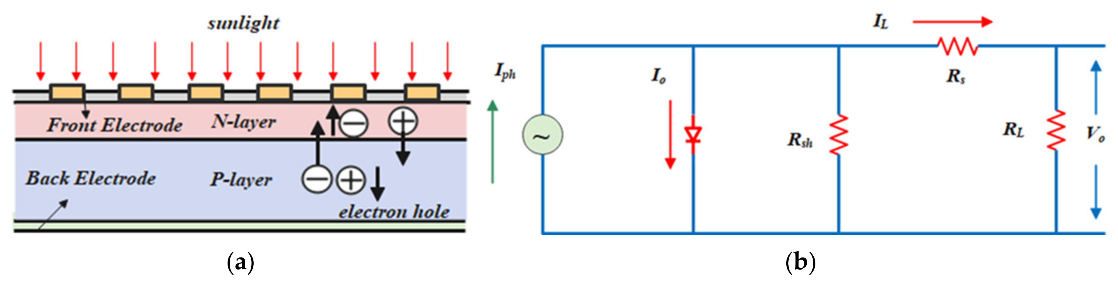
Solar cells harness radiation through the “photovoltaic effect” to convert it into electric power [21]. This phenomenon entails the generation of electron-hole pairs (EHPs) within solar cells upon exposure to sunlight, inducing the formation of an internal electric field at a PN junction. Consequently, the electron-hole pairs migrate to their respective regions within the solar cells, driven by the built-in electric field. As electrons move towards the n-type region and the holes migrate towards the p-type one, a current flow ensues. Figure 1a illustrates the principle of the photovoltaic effect.

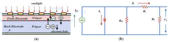
Figure 1. Mathematical modeling of photovoltaic cells: (a) photovoltaic effect; (b) equivalent circuit model.

Due to the optical limitations of the laying area, the scale of a PV system is increased by connecting more photovoltaic cells in series and in parallel. Irradiance and temperature are two important indicators of the photoelectric conversion process. In order to simplify the analysis process of the overall system, an individual PV cell is taken as the research object, and mathematical models are established for evaluating the output characteristics of photovoltaic cells under different conditions.

Ideally, considering the internal losses of the PV cell, the model of the PV cell could be considered as an equivalent circuit model consisting of a constant current source with a paralleled diode [22]. As shown in Figure 1b, I_ph represents the photocurrent, I_L is the output current of the photovoltaic cell, v_o is the output voltage of the photovoltaic cell, I_o represents the dark current flowing through the diode, R_sh is the shunt resistance, and D represents the diode.

Using Kirchhoff’s laws, the mathematical model of the PV cell can be refined as follows [23]:

$$I=I_{ph}-I_o{\exp }^{{\displaystyle \frac{q\left(V_{pv}+R_{s}I\right)}{AKT}}}-{\displaystyle \frac{V_{pv}+R_s{I}_L}{R_{sh}}}$$

(1)

where K is the Boltzmann constant and A represents the ideality factor.

2.2. Analysis of Photovoltaic Output Characteristics

The shading problem of PV systems mainly originates from factors such as dust coverage, cloud cover, and building obstruction. The power generation performance is strongly influenced by both nonlinear factors and external environmental conditions. When under the shadow, the original single-peak power characteristic curve may transfer into a complex multi-peak pattern. As the degree of shadowing deepens, the tracking process of the global maximum power point (GMPP) becomes increasingly tricky, which may result in the actual tracked power point tending to a local maximum power point (LMPP). This change directly leads to a significant reduction in the efficiency of PV power generation, which, in extreme cases, can be reduced to as low as 30% of the original efficiency. In addition, such shadowing conditions can induce ”hot spots” which can potentially damage PV cells [24].

The second figure (Figure 2) depicts the output performance characteristic curve of the PV power generation system under uniform light environments. Meanwhile, it reveals the output performance characteristic curve of the PV power system when it encounters a shading condition.

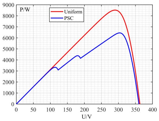
Figure 2. Output characteristics of photovoltaic cells under uniform radiance and PSC.

Traditional MPPT techniques are designed for uniform radiation conditions. However, under shading conditions, the output characteristic curve of the PV cell deviates from single-peak to multi-peak. As illustrated in Figure 2, the P-U curve of the photovoltaic cell contains one global maximum power point (GMPP) and several local maximum power points (LMPPs). The presence of diodes causes batteries with lower current levels to be continuously activated as the voltage levels increase. In this scenario, the traditional MPPT technology might fall into the LMPP and fail to reach the GMPP. Therefore, a key determinant of improving the power generation efficiency is the ability to track the GMPP.

3. MPPT Control Method Based on IHPO Algorithm

By observing the behavior of predators (such as lions, leopards, and wolves) and prey (such as stag and gazelles), ref. [25] proposed a new swarm optimization algorithm called Hunter–Prey Optimization (HPO). The procedure of HPO involves the following position updates for both the prey and hunter populations: the former adopts an escape mechanism that converges to the optimal position, while the latter follows the hunters’ tracking path, updating through hunting behavior.

Initially, the overall individuals are randomly assigned to {$\overrightarrow{x}$} = {$\overrightarrow{x}$₁, $\overrightarrow{x}$₂, ..., $\overrightarrow{x}$₃}, and, subsequently, the objective function of all members in the population is evaluated as {$\overrightarrow{O}$} = {$\overrightarrow{O}$₁, $\overrightarrow{O}$₂, ..., $\overrightarrow{O}$₃}. Aligning with its inspiration, this algorithmic approach controls and guides the population effectively within the search space through a series of meticulously designed rules and strategies running iteratively. In a single iteration, the position of each individual in the swarm would be updated following the algorithmic rules, while the objective function evaluates the new position. Every iteration facilitates the optimization of the solution, and this iterative process persists until the algorithm converges. The initial positions of all population members are generated randomly within the search space by employing Equation (2), as follows:

$$x_1=rand \left(1,d\right)·\left(u_b-l_b\right)+l_b$$

(2)

Here, x_i denotes the initial positions of either the hunter or prey population, l_b represents the minimum value (lower bound) of the problem variable, u_b represents the maximum value (upper bound) of the problem variable, and d represents the number of problem variables (dimensions). Equation (3) defines the lower and upper bounds of the search space. It is important to note that the upper and lower limits of all variables within a given problem may be identical or distinct.

$$l_b=\left[l_{b1},l_{b2},I,l_{bd}\right],u_b=\left[u_{b1},u_{b2},I,u_{bd}\right]$$

(3)

After generating the initial population and determining the position of each agent, the fitness value for each solution is calculated using the objective function O_i = F($\overrightarrow{x}$). F($\overrightarrow{x}$) can be the maximum (efficiency, performance, etc.) or the minimum (cost, time, etc.). The search algorithm usually consists of the following two steps: exploration and development. Exploration is when algorithms tend to behave highly randomly, so the solution changes significantly. Significant changes in solutions encourage hunters to explore the search space further and discover its promising areas. After discovering promising areas, the randomness must be reduced so that the algorithm can search around the promising areas.

Regarding the search mechanism of the hunter, Equation (4) provides the mathematical formulation, as follows:

$$x_{i,j}\left(t+1\right)=x_{i,j}\left(t\right)+0.5\left[2CZ{P}_{pos\left(j\right)}-x_{i,j}\left(t\right)+\left(2\left(1-C\right)Z\mu j-x_{i,j}\left(t\right)\right)\right]$$

(4)

where x(t) is the current position of the hunter, x(t + 1) is the next iteration position of the hunter, P_pos is the position of the prey, µ is the mean value of all positions, j is the index of dimension, and Z is the adaptive parameter calculated by Equation (5).

$$P=\overrightarrow{R_1}<C;IDX=\left(P==0\right)$$

(5)

$$l_b=\left[l_{b1},l_{b2},I,l_{bd}\right],u_b=\left[u_{b1},u_{b2},I,u_{bd}\right]$$

(6)

Here, ${\overrightarrow{R}}_1$ and ${\overrightarrow{R}}_3$ are random vectors within [0, 1], P is an index value for ${\overrightarrow{R}}_1<C$, $R2$ is a random number within [0, 1], IDX is an index value for the vector $\overrightarrow{R}1$ that satisfies the condition P equals to 0, and C is a balance parameter between exploration and exploitation, with its value decreasing from 1 to 0.02 during the iteration process, which is calculated as follows:

$$C=1-iter\left({\displaystyle \frac{0.98}{MaxIt}}\right)$$

(7)

where iter denotes the current iteration number and MaxIt denotes the maximum number of iterations. The position of the prey, P_pos, is determined by, firstly, the mean of all positions according to Equation (8), as follows:

$$\mu ={\displaystyle \frac{1}{n}}{{\displaystyle \sum }}_{i=1}^n\overrightarrow{x_i}$$

(8)

and subsequently the Euclidean distance of each search agent to this mean position according to Equation (9), as follows:

$$D_{euc}\left(i\right)={({{\displaystyle \sum }}_{j=1}^d{\left(x_{i,j}-{\mu }_j\right)}^2)}^{{\displaystyle \frac{1}{2}}}$$

(9)

The search agent with the maximum distance from the average position is considered as the prey. If the algorithm finds the maximum distance between the search agent and the mean position µ at every iteration, it may exhibit delayed convergence. In a hunting scenario, once the hunter captures the prey, the prey dies, and the hunter must move to a new location to capture the next prey. A decreasing mechanism is proposed to mitigate this issue as described by Equation (10), as follows:

$$k_{best}=round\left(C\times N\right)$$

(10)

where N denotes the number of search agents. By modifying Equation (9), the position of the prey P_pos is calculated using Equation (11), as follows:

$$\overrightarrow{P_{pos}}=\overrightarrow{x_i}$$

(11)

At the beginning of the algorithm, the value of k_best is equal to N. Therefore, the search agent farthest from the average position µ is selected as the prey and is captured by the hunter. If the best safe position is assumed to be the best global position, as it would increase the chances of survival for the prey, the hunter may select a different prey. Equation (12) is used to update the position of the prey, as follows:

$$x_{i,j}\left(t+1\right)=T_{pso\left(j\right)}+CZ\cos (2\pi R_4)\times \left(T_{pso\left(j\right)}-x_{i,j}\left(t\right)\right)$$

(12)

In the Equation above, x(t) represents the current position of the prey, while x(t + 1) denotes the subsequent iterated position. T_pos signifies the globally optimal position, whereas Z corresponds to the adaptive parameter calculated using Equation (4). R₄ is a random variable uniformly distributed within the range [−1, 1]. The balance parameter, C, which governs the trade-off between exploration and exploitation, is progressively reduced during the algorithmic iterations and computed using Equation (6). The cos function and input parameters facilitate the prey’s next position to approach the global optimal position at different radii and angles, thereby enhancing the algorithm’s performance during the exploitation phase.

In order to select the hunter and prey, we propose Equation (13) by integrating Equations (4) and (12), as follows:

$$x_i\left(t+1\right)=\left\{\begin{array}{l}{x}_1\left(t\right)+0.5\left[\left(2CZ{P}_{pos\left(j\right)}-x_i\left(t\right)+\left(2\left(1-C\right)Z\mu \left(j\right)\right)-x_i\left(t\right)\right)\right]\hspace{1em}if R_5<\beta \\ T_{pos}+CZ\left(2\pi R_4\right)\times \left(T_{pos}-x_i\left(t\right)\right)\hspace{1em}\hspace{1em}\hspace{1em}\hspace{1em}\hspace{1em}\hspace{1em}\hspace{1em}else\end{array}\right.$$

(13)

where R₅ is a random number within the range of [0, 1] and β is a tuning parameter with a value of 0.1 in this paper. If the value of R₅ is less than β, the search agent is considered a hunter, and its next position will be updated using Equation (13). Conversely, if the value of R5 is greater than β, the search agent is regarded as prey, and its next position will be updated using Equation (13).

Based on the description above, an improved position updating method is proposed [26], which incorporates a spiral search strategy into the existing algorithm, coupled with a preliminary optimization of the acceleration algorithm and a subsequent refinement of the convergence criteria. To some extent, the improved part reduces the overall search time and enhances the convergence rate, thereby mitigating the errors encountered during the optimization process. The hunter determines the position update methodology through the parameter Δx, which guides the movement towards the food source along a spiral trajectory. Equations (14) and (15) present the mathematical model of this process, as follows:

$$x_i\left(t+1\right)=\left\{\begin{array}{l}{x}_{best}+r\times \left(x_{best}-x_i\left(t\right)\right)+m\times \left(x_{best}-x_i\left(t\right)\right) i=1\\ x_{best}+r\times \left(x_{i-1}\left(t\right)-x_i\left(t\right)\right)+m\times \left(x_{best}-x_i\left(t\right)\right) i=1,2,\cdots ,N\end{array}\right.$$

(14)

$$m=2e^{r_1{\displaystyle \frac{MaxIt-iter+1}{MaxIt}}}\cdot \sin (2\pi r_1)$$

(15)

In Equation (15), r denotes a uniformly distributed random number within the range [0, 1], m denotes the inertial weight, and r₁ denotes a uniformly distributed random number within the range [0, 1]. When iter or MaxIt are less than the randomly generated number, all individuals are assigned a new random position within the entire search space as their reference position, as follows:

$$x_{rand}=l_b+m\times \left(u_b-l_b\right)$$

(16)

$$x_i\left(t+1\right)=\left\{\begin{array}{l}{x}_{rand}+r\times \left(x_{rand}-x_i\left(t\right)\right)+m\times \left(x_{rand}-x_i\left(t\right)\right) i=1\\ x_{rand}+r\times \left(x_{i-1}\left(t\right)-x_i\left(t\right)\right)+m\times \left(x_{rand}-x_i\left(t\right)\right) i=1,2,\cdots ,N\end{array}\right.$$

(17)

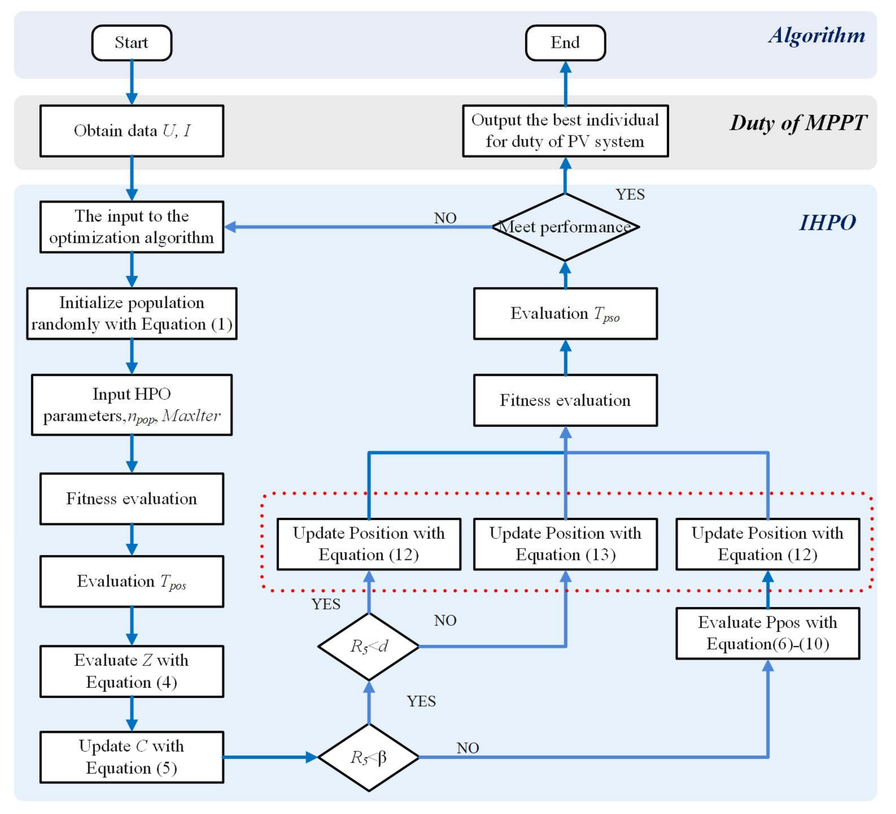
The operational process of the algorithm is illustrated in Figure 3, whose working principle is detailed as follows.

Figure 3. Improved control method flowchart.

First of all, the current and voltage data of a PV system are collected as the algorithm’s input. Hunters and individual prey are considered as duty cycle signals required by the PV system to initialize the swarm.

Next, an individual space is setup with individuals x_i generated randomly within it, and the upper and lower bounds, l_b and u_b, of the space are thereby defined. When the hunter detects the target region, randomness during the hunting process is reduced, and the search mechanism x_i,j(t + 1) of the hunter is defined for that region.

According to the parameters of the IHPO algorithm, the balance parameter C between exploration and exploitation is calculated during the iteration. The distances between all search agents of the prey and the mean position are calculated, and the fitness function is applied to determine whether the result meets the requirements.

Based on the limiting values, the position of the prey or the hunter is updated, and the hunter’s position update method is determined based on Δx. Subsequently, the re-evaluation of the fitness value of the algorithm is executed. Finally, the process ends when the algorithm reaches the maximum number of iterations or satisfies the fitness requirements.

4. Simulation Analysis

In order to verify the effectiveness of the proposed method, a PV system based on the IHPO algorithm and other group optimization algorithms for MPPT is constructed. As shown in Figure 4, the system comprises a PV array, a DC–DC boost circuit, and an MPPT controller. Specifically, the power supply side encompasses five sets of PV arrays, denoted as PV₁–PV₅. Each array’s radiation intensity, G₁–G₅, varies under distinct shading conditions. The voltage and current data of the five PV arrays are gathered and used to optimize the maximum power point of the photovoltaic system through different group optimization algorithms. The output of an MPPT algorithm is transferred into the PWM driving signals of the IGBT.

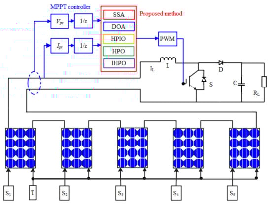
Figure 4. Schematic diagram of the operating structure of the photovoltaic system.

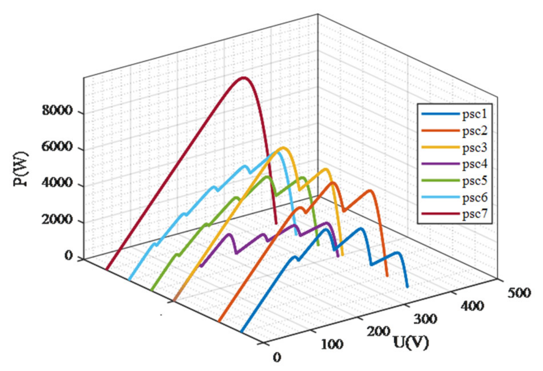
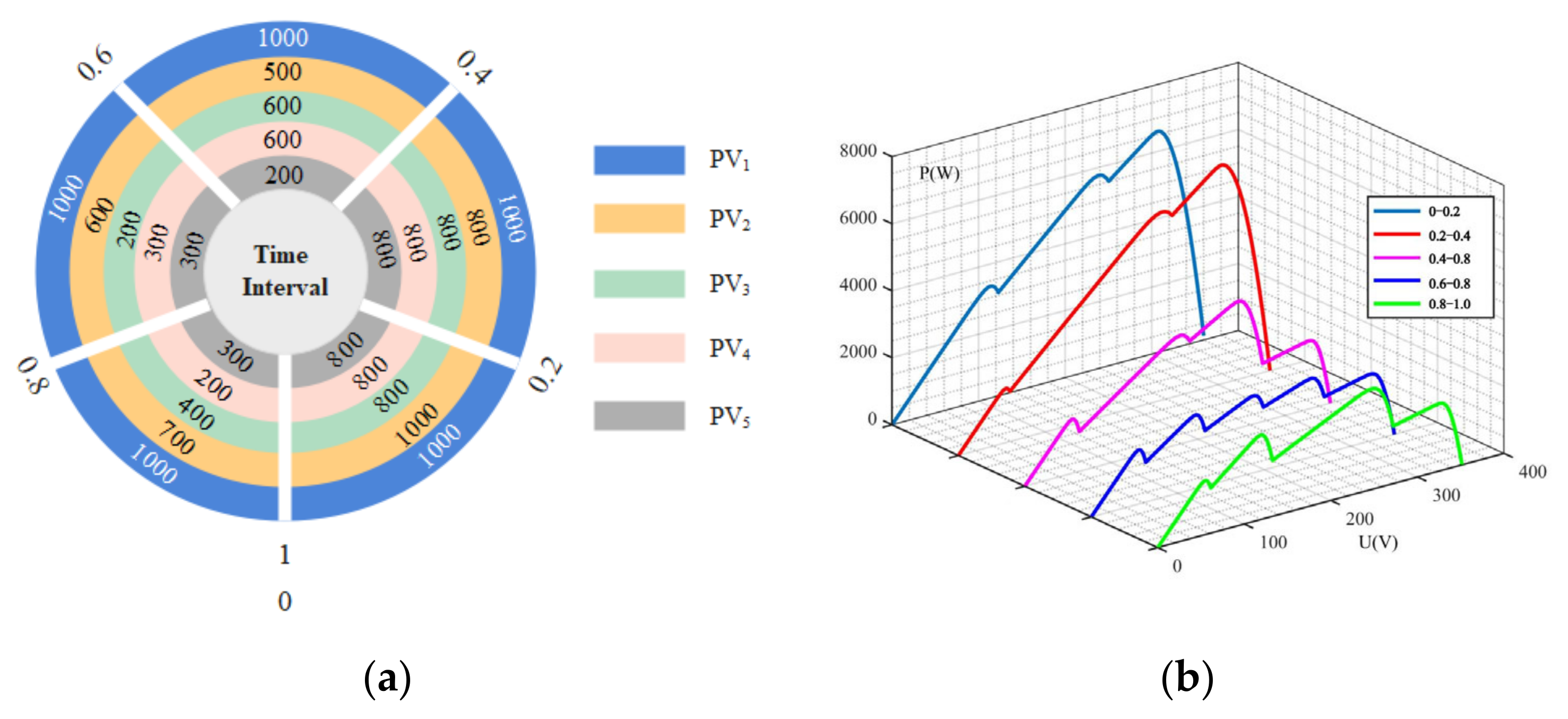
The pertinent parameters of the PV cell are presented in Table 1. This work constructed seven static shading conditions, with the specific details outlined in Table 2, to compare the performances of five different control methods under complex shading conditions. The corresponding output characteristic curve (P-U) is displayed in Figure 5. Additionally, a dynamic shading condition is constructed, with its parameter setup illustratively plotted in Figure 6.

Table 1. Parameters of the Soltech 1STH-215-P PV module.

Item	Value	Item	Value
Pmax (W)	213.15	Impp (A)	7.35
Voc (V)	36.3	Series-connected cells	60
Vmax (V)	29	Temperature coefficient of Voc (%/°C)	−0.361
Isc (A)	7.84	Temperature coefficient of Isc (%/°C)	0.102

Table 2. Radiation values of the five PV arrays under seven static shading conditions.

Radiance (W/m2)	PV1	PV2	PV2	PV4	PV5	MPP (W)
PSC1	1000	1000	1000	1000	1000	8517
PSC2	1000	800	700	600	500	4900
PSC3	1000	800	700	600	400	4530
PSC4	1000	800	400	300	200	2831
PSC5	1000	1000	1000	1000	500	6789
PSC6	1000	1000	1000	800	500	5944
PSC7	1000	1000	800	500	200	4885

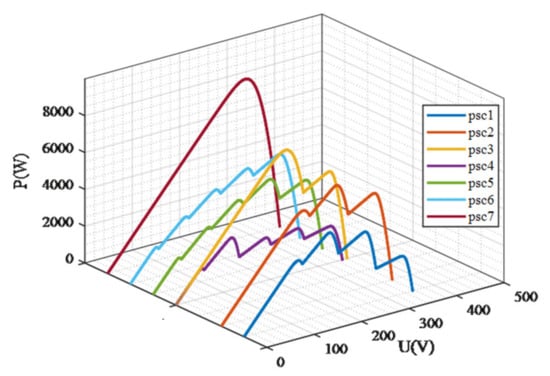
Figure 5. P-U characteristic curve of the photovoltaic system under different shading conditions.

Figure 6. Dynamic shading condition setup: (a) radiation plot of the photovoltaic arrays in different time intervals; (b) P-U characteristic curve.

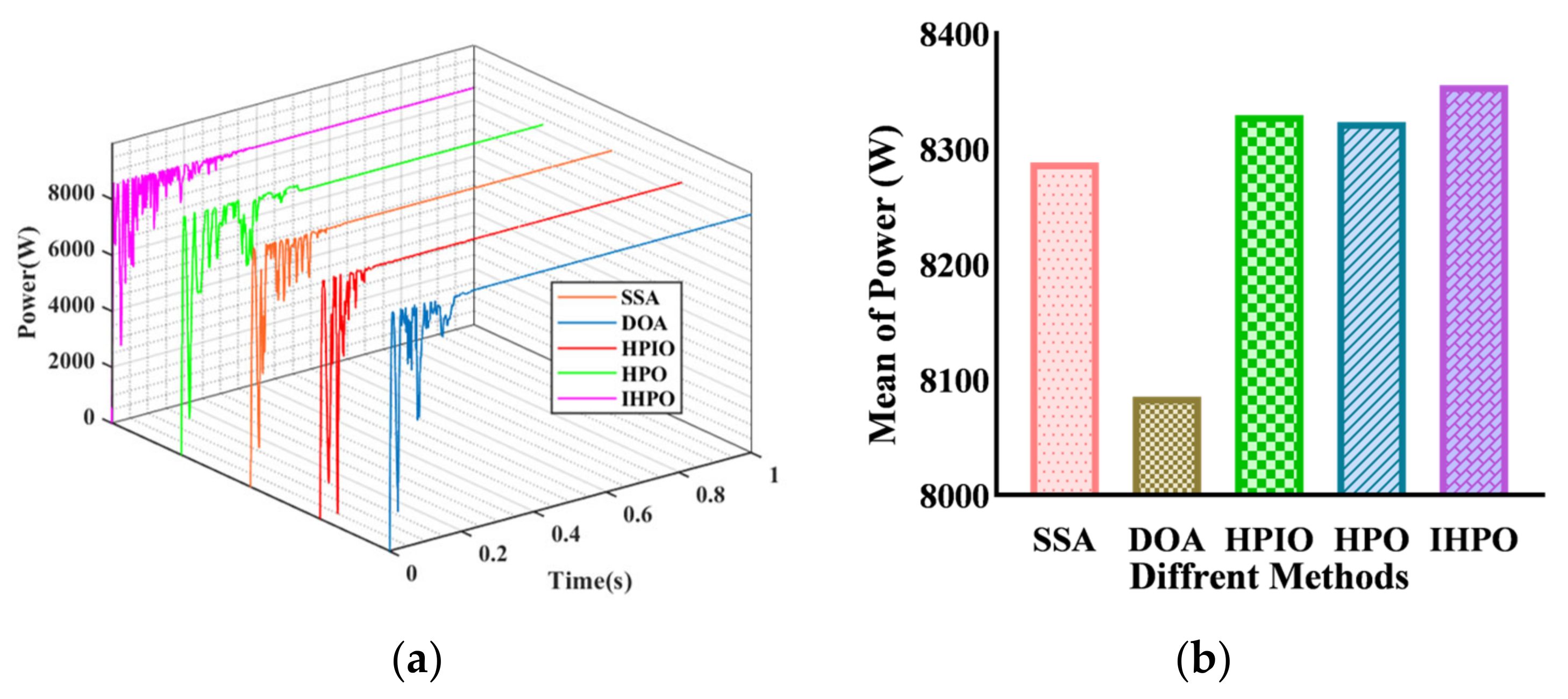
Under PSC1, it can be observed from Figure 7 that the proposed control method achieved 100% efficiency tracking within 0.179 s, with the shortest tracking time among the five algorithms considered. In contrast, the tracking times for the other four control methods were found to be 0.397 s, 0.327 s, 0.382 s, and 0.227 s, respectively. The DOA algorithm demonstrated the poorest performance, exhibiting a tracking efficiency of 97.45%, while the remaining algorithms recorded complete tracking efficiency. Notably, the proposed algorithm was able to achieve a 57.51% reduction in tracking time relative to the SSA algorithm. The HPO and IHPO algorithms were found to have shorter tracking times, indicating certain advantages in the MPPT control process. The algorithm demonstrated strong search capabilities, and the improved method exhibited a discernible degree of enhancement relative to the original algorithm.

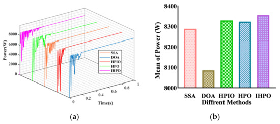
Figure 7. Tracking performances of different algorithms under PSC1: (a) output power curve; (b) average of power.

Under PSC2, the global maximum power is determined to be 4900 W (Figure 8). The Squirrel Search Algorithm achieved a 100% success rate in capturing a power of 4527 W with a tracking efficiency of 92.39% at a completion time of 0.3921 s. Similarly, the Directional Optimization Algorithm (DOA) method yielded a steady-state power of 4523 W at a completion time of 0.255 s, with a tracking efficiency of 92.3%. The Hybrid Particle-Inheritance Optimization (HPIO) method accomplished a tracking time of 0.206 s and a steady-state power of 4521 W. Both the Hybrid Particle Optimization (HPO) and Improved.

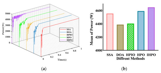
Figure 8. Tracking performances of different algorithms under PSC2: (a) output power curve; (b) average of power.

The Hybrid Particle Optimization (IHPO) control methods demonstrated a tracking efficiency of 98.4%, with response times of 0.134 s and 0.064 s, respectively. The proposed method exhibited a notable advantage in the tracking time.

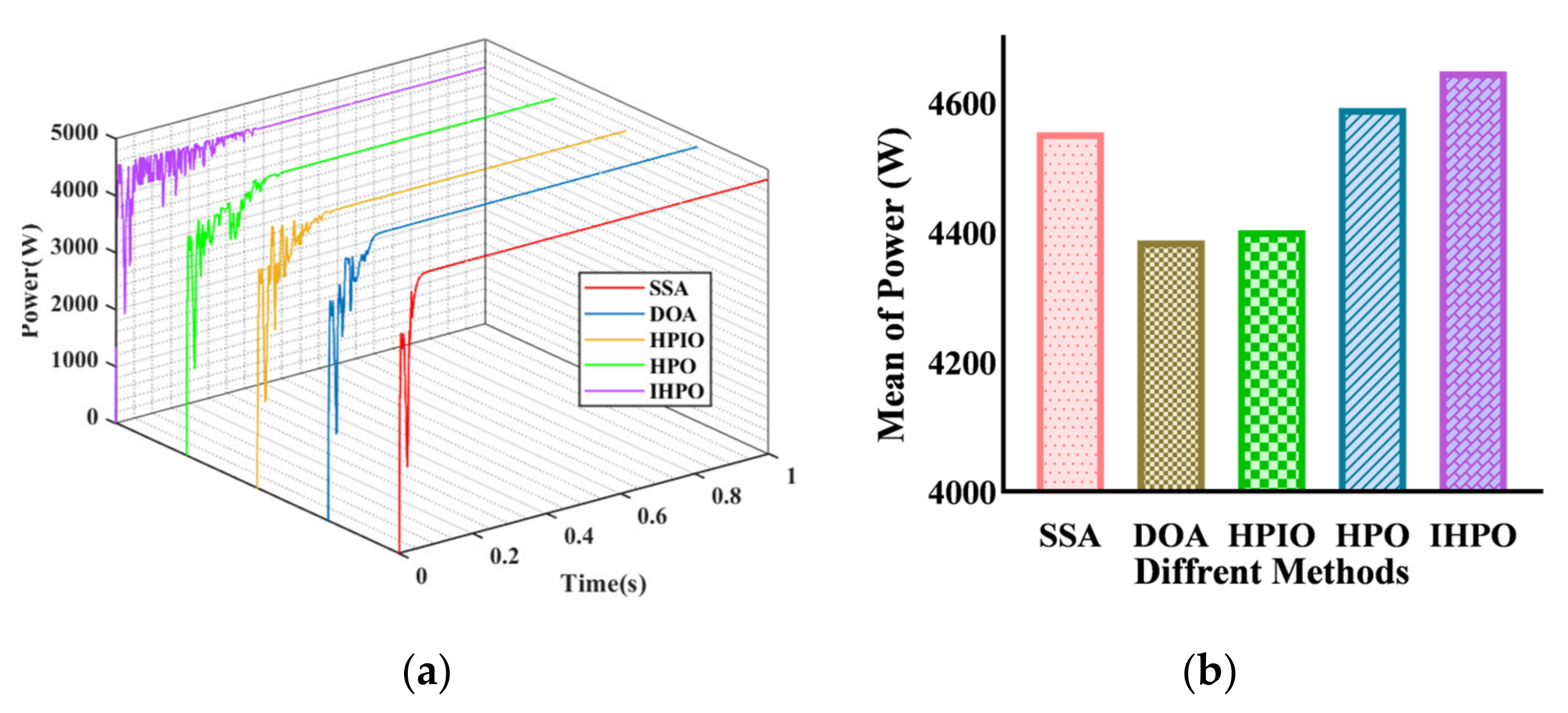
Under the PCS3, the global maximum power output of the system amounts to 4530 W (Figure 9). The Squirrel Search Algorithm (SSA) control method captures the maximum power point within 0.372 s, while the Directional Optimization Algorithm (DOA) control method attains a steady-state power output of 4493 W within 0.278 s. The remaining three control methods exhibit the ability to track the maximum power point of the photovoltaic system, with tracking times of 0.227 s, 0.324 s, and 0.21 s, respectively. The proposed control method substantially reduces tracking time by 43.5%, 7.4%, and 35.2% compared to the SSA, HPIO, and Improved Hybrid Particle Optimization (IHPO) control methods, respectively. The improved method manifests a significant enhancement in tracking time, thereby underscoring the necessity of the enhancement strategy.

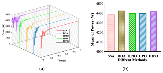
Figure 9. Tracking performances of different algorithms under PSC3: (a) output power curve; (b) average of power.

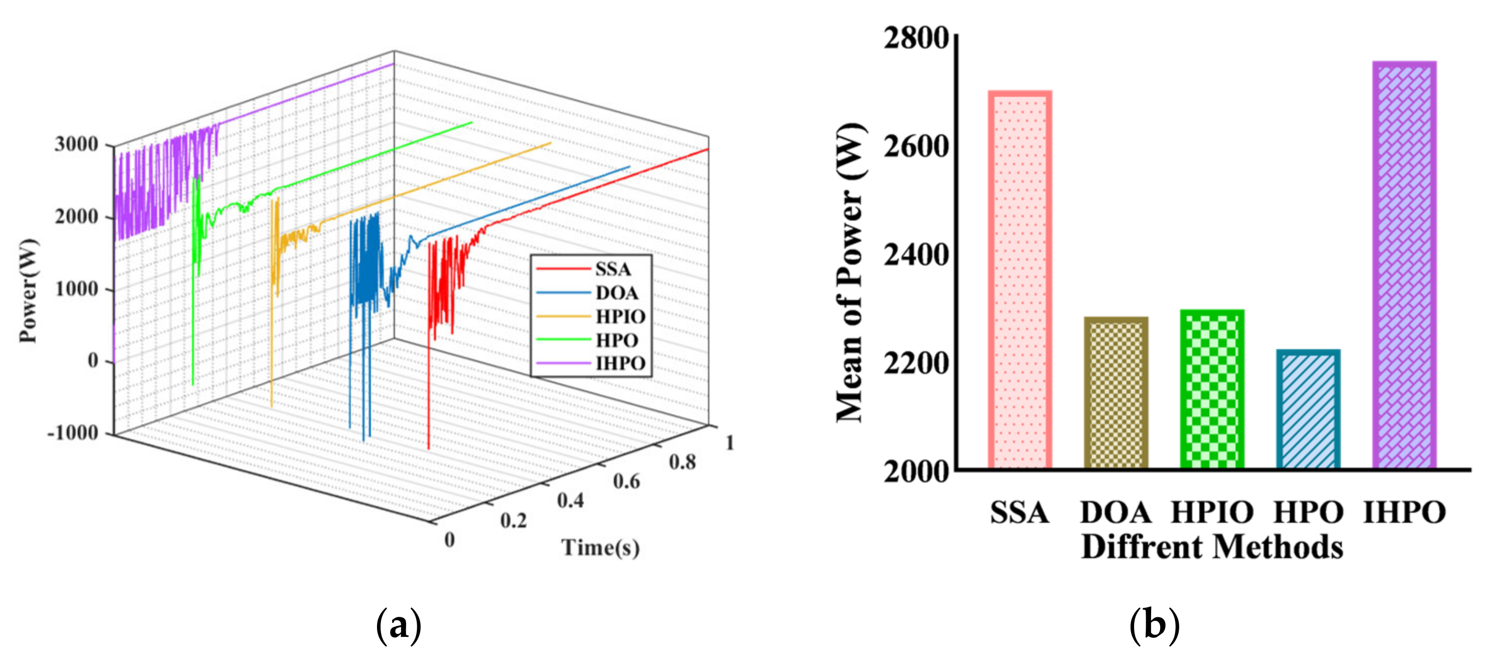
Under the fourth PSC, the global maximum power point of the system is 2831 W (Figure 10). The control methods capable of capturing the maximum power point are the SSA and IHPO control methods, but the former has a longer tracking time of 0.407 s, while the proposed control method completes tracking at 0.203 s. The steady-state powers of the other three control methods (DOA, HPIO, and HPO) are 2285 W, 2317 W, and 2317 W, respectively. The tracking times are 0.278 s, 0.227 s, and 0.263 s, respectively. Through comprehensive comparison, it is known that the proposed method has the shortest tracking time while ensuring tracking efficiency.

Figure 10. Tracking performances of different algorithms under PSC4: (a) output power curve; (b) average of power.

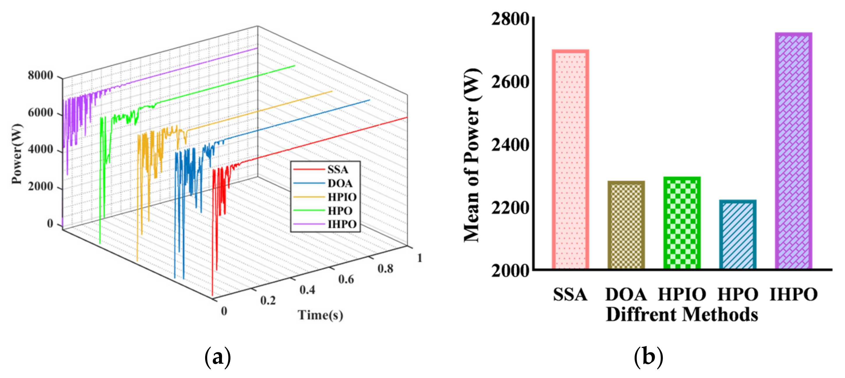
Under the fifth PSC, the global maximum power of the system is 6789 W (Figure 11). Both the DOA and the proposed control method can capture the maximum power point. The tracking time of the former is 0.3507 s, while the latter’s tracking time is 0.153 s. The tracking powers of the other three controls are 6780 W, 6328 W, and 6774 W, with tracking times of 0.3507 s, 0.256 s, and 0.259 s, respectively. The proposed control method exhibits good control performance in terms of the tracking time and tracking efficiency.

Figure 11. Tracking performances of different algorithms under PSC5: (a) output power curve; (b) average of power.

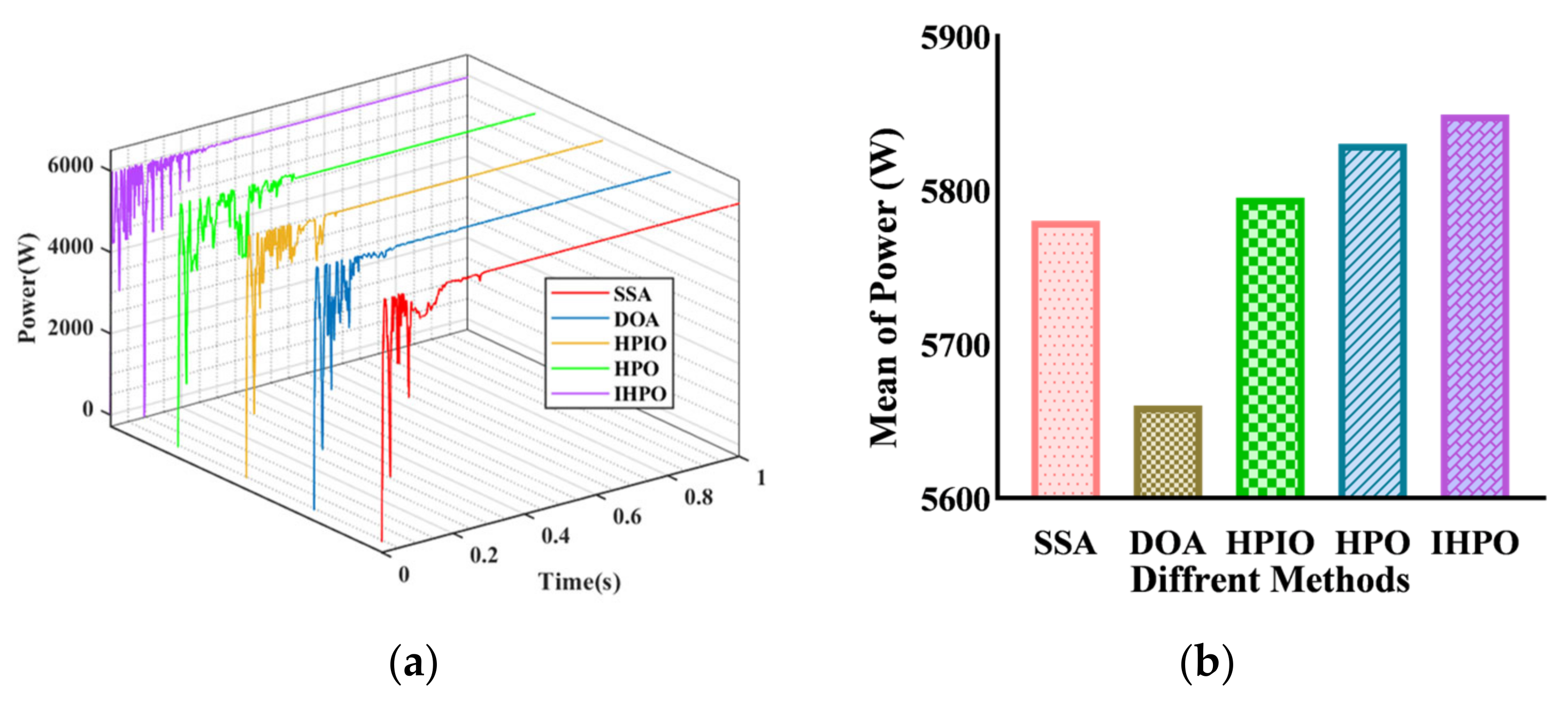
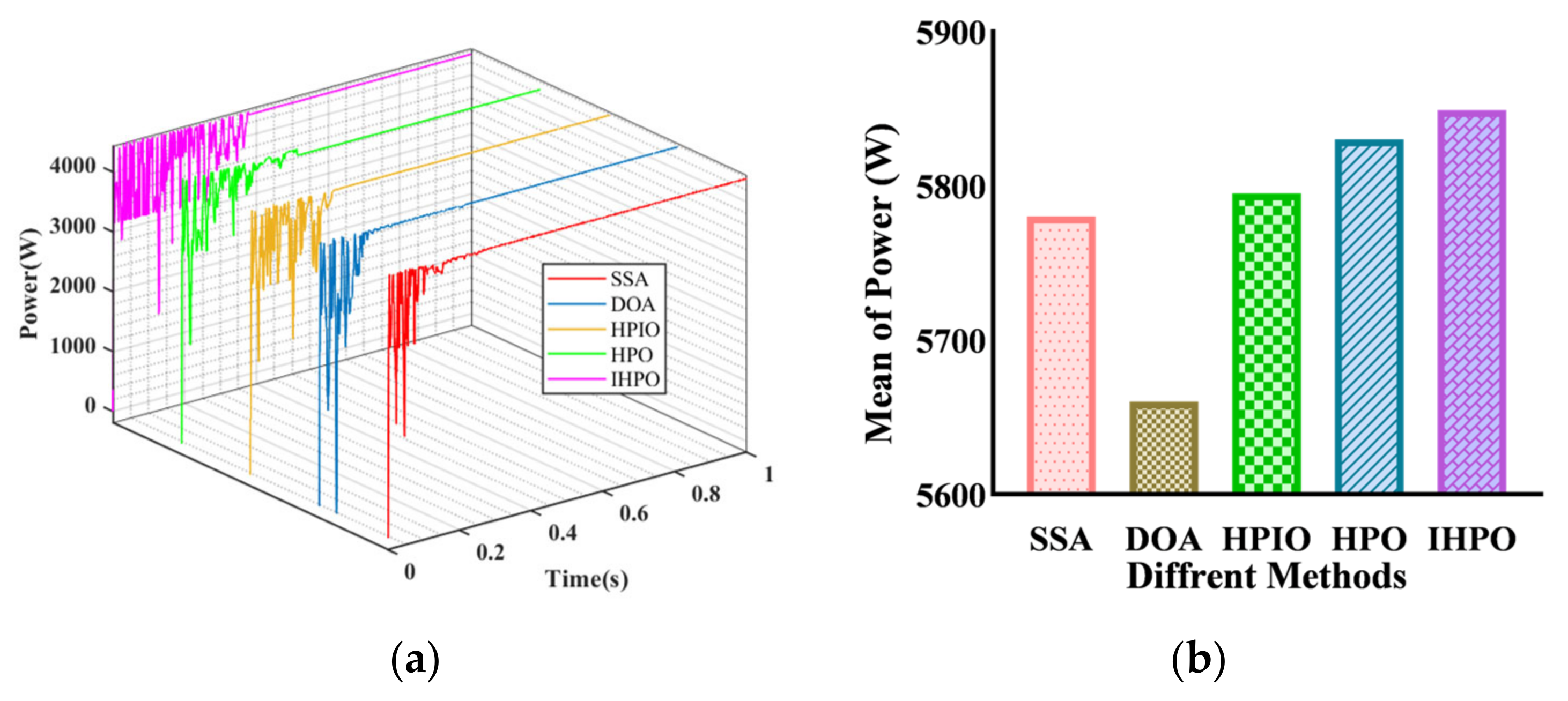
In the sixth scenario, the global maximum power of the system is 5944 W (Figure 12). The tracking efficiency of the DOA control method is 5819 W, which does not fully capture the global maximum power point. The other four control methods can all achieve maximum power tracking, with tracking times of 0.337 s, 0.357 s, 0.36 s, and 0.182 s for the SSA, HPIO, HPO, and IHPO control methods, respectively. The proposed control method has a shorter tracking time, which is reduced by 49.4% compared to the original HPO algorithm.

Figure 12. Tracking performances of different algorithms under PSC6: (a) output power curve; (b) average of power.

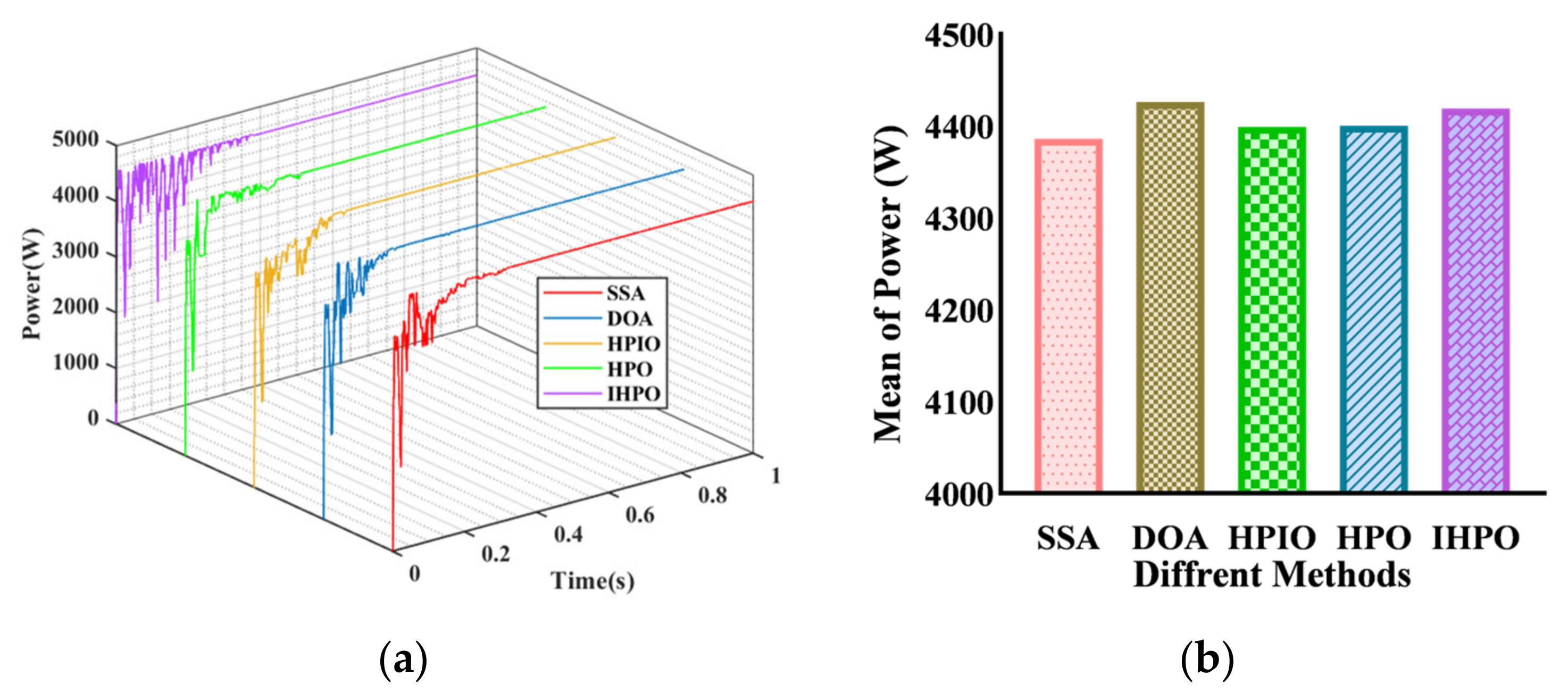
In the seventh shading condition, the global maximum power of the system is determined to be 4385 W (Figure 13). Both the Squirrel Search Algorithm (SSA) and the proposed algorithm are capable of capturing the maximum power point, with respective tracking times of 0.379 s and 0.18 s. However, the other three control methods fail to achieve adequate power tracking, with tracking powers of 4280 W, 4361 W, and 4370 W, and corresponding tracking times of 0.336 s, 0.357 s, and 0.36 s. It can be inferred through comprehensive comparison that the proposed method demonstrates superior performance across various output performance metrics.

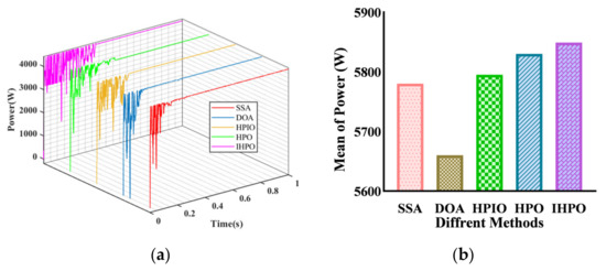
Figure 13. Tracking performances of different algorithms under PSC7: (a) output power curve; (b) average of power.

In the dynamic shading condition, time-varying behavior in the five solar panels was implemented deliberately to assess the tracking performance of different control methods under dynamic shadow conditions (Figure 14). Throughout the tracking process, the global maximum power point varied temporally. Analysis of the output curve reveals that the Directional Optimization Algorithm (DOA) tracking method failed and exhibited significant instability during operation. The Squirrel Search Algorithm (SSA) control method also showed instability, with the global maximum power point changing within 0.4 s, yet the algorithm had not reached a steady state. The Hybrid Particle Optimization (HPO) control method displayed minor fluctuations and instability during operation. The Hybrid Particle-Inheritance Optimization (HPIO) control method successfully captured the maximum power during the initial power conversion. In contrast, the proposed control method reached the maximum power point before 0.2 s and subsequently generated a smooth output curve. Overall, the effectiveness of the Improved Hybrid Particle Optimization (IHPO) control method was affirmed, as it adeptly managed photovoltaic system (PSC) switching.

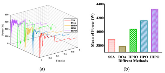
Figure 14. Tracking performances of dynamic shading condition: (a) output power curve; (b) average of power.

This study analyzed eight cases to assess the efficacy of various control methods in adapting to diverse shadow conditions. The findings highlight the proposed control strategies’ capability to manage extensive and localized shadow areas adeptly. Nonetheless, the Squirrel Search Algorithm (SSA) control method displays prolonged tracking times attributable to constraints inherent in its search mechanism. Additionally, the Directional Optimization Algorithm (DOA) control method exhibits subpar performance in scenarios characterized by significant dynamic shadow fluctuations. While the Hybrid Particle-Inheritance Optimization (HPIO) control method mitigates some shortcomings observed in the former approaches, it remains marginally inferior to the latter alternatives. Despite the general suitability of the Hybrid Particle Optimization (HPO) algorithm across most scenarios, occasional tracking failures may occur, potentially stemming from limitations in the employed optimization methodologies. Introducing novel strategies could enhance the algorithm convergence. Conversely, the Improved Hybrid Particle Optimization (IHPO) algorithm showcases remarkable tracking efficiency, achieving a success rate exceeding 98%, even amidst dynamic shadow transitions. The output performance of the five methods across varied shadow conditions is summarized in Table 3.

Table 3. Comparison table of the output parameters of the five algorithms.

Cases	Algorithm	MPP (W)	Ppv (W)	Tracking Speed (s)	MPPT Efficiency (%)
PSC1	SSA	8517	8517	0.397	100
	DOA		8300	0.327	97.45
	HPIO		8517	0.382	100
	HPO		8517	0.227	100
	IHPO		8517	0.178	100
PSC2	SSA	4900	4527	0.392	92.39
	DOA		4523	0.225	92.3
	HPIO		4521	0.206	92.26
	HPO		4821	0.134	98.38
	IHPO		4821	0.064	98.38
PSC3	SSA	4530	4530	0.372	100
	DOA		4493	0.278	99.18
	HPIO		4530	0.227	100
	HPO		4530	0.324	100
	IHPO		4530	0.21	100
PSC4	SSA	2831	2831	0.407	100
	DOA		2285	0.289	80.71
	HPIO		2317	0.278	81.84
	HPO		2317	0.263	81.84
	IHPO		2831	0.203	100
PSC5	SSA	6789	6789	0.351	100
	DOA		6789	0.312	100
	HPIO		6328	0.259	93.21
	HPO		6774	0.256	99.77
	IHPO		6789	0.153	100
PSC6	SSA	5944	5944	0.337	100
	DOA		5944	0.342	100
	HPIO		5819	0.357	97.89
	HPO		5944	0.361	100
	IHPO		5944	0.182	100
PSC7	SSA	4885	4885	0.379	100
	DOA		4280	0.326	87.62
	HPIO		4361	0.251	89.27
	HPO		4378	0.224	89.62
	IHPO		4885	0.185	100

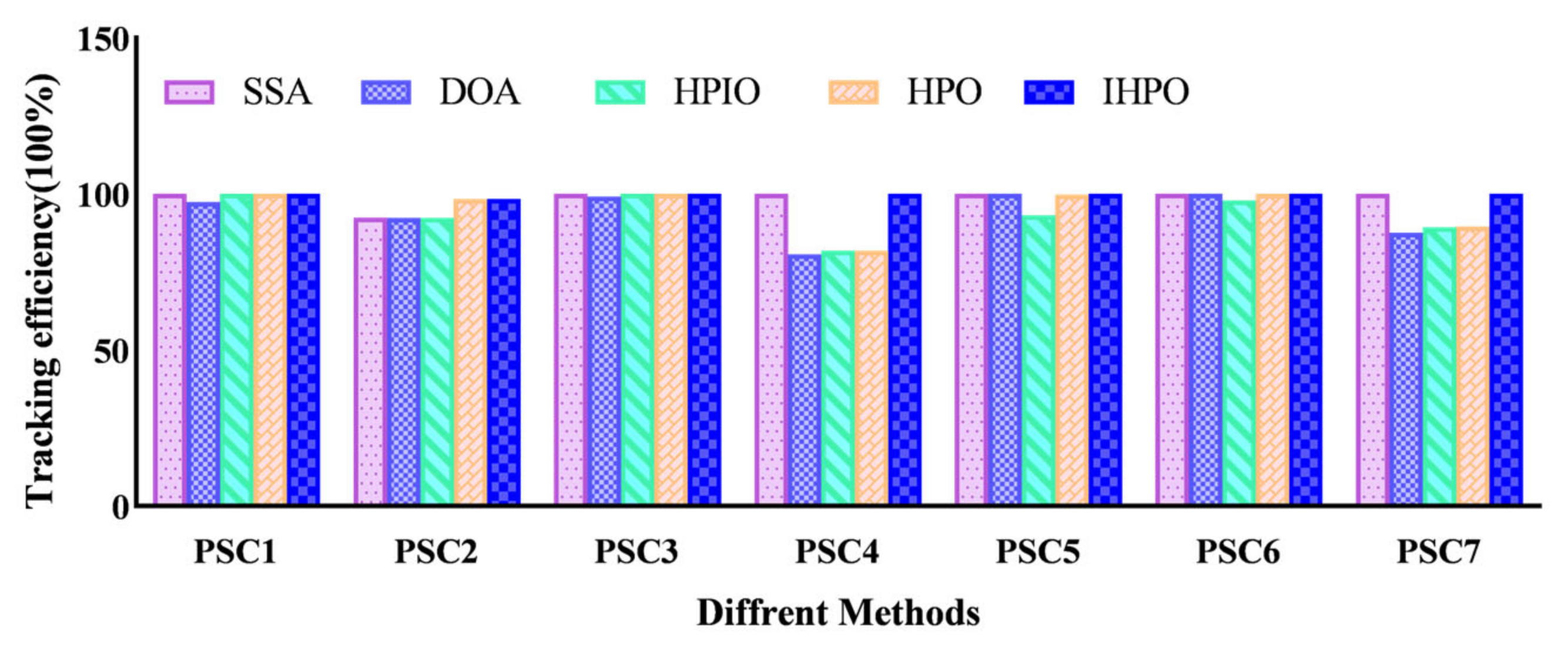
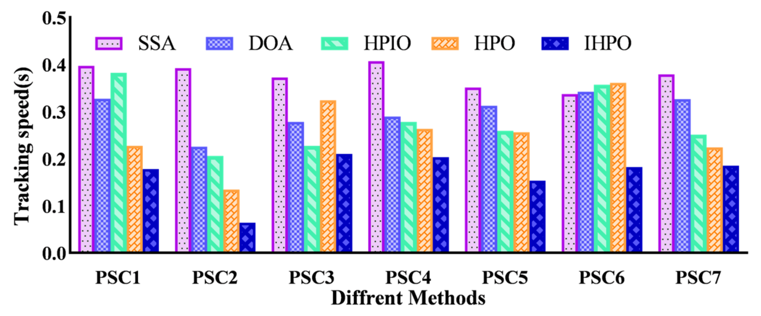
This comprehensive analysis delved into the power generation dynamics of photovoltaic systems, scrutinizing their behavior under both uniform and varied shading conditions. Utilizing histograms, the study synthesized data on the response speed and tracking efficiency across various control methods, providing a visual representation of their performance nuances (as illustrated in Figure 15 and Figure 16, respectively). The results underscore the efficacy of the proposed method, which exhibits remarkable tracking capabilities characterized by a 100% efficiency and swift response times, outperforming its counterparts.

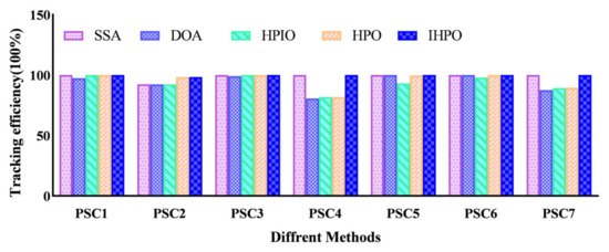
Figure 15. The histogram of the tracking efficiency on the simulation platform.

Figure 16. The histogram of tracking speed on the simulation platform.

Specifically, the proposed control strategy showcases unparalleled efficiency in reaching a steady state, as evidenced by its remarkably short tracking time of 0.064 s under the second shading scenario—a noteworthy 83.7% reduction compared to the Squirrel Search Algorithm (SSA). Moreover, the proposed method demonstrates commendable responsiveness even in dynamic shading conditions, achieving a response time of approximately 0.2 s. This swift adaptation ensures an optimized approach to maximizing the photovoltaic system’s power output, thereby enhancing the overall operational efficiency.

Additionally, the comparative analysis sheds light on the limitations of alternative control methods. For instance, the SSA algorithm’s longer tracking times highlight its inefficiency in swiftly adapting to dynamic shading conditions. Meanwhile, the proposed method’s superior performance is underscored by its ability to maintain high tracking efficiency while minimizing response times, positioning it as a promising solution for optimizing photovoltaic system performance across varying environmental conditions.

5. Experimental Verification

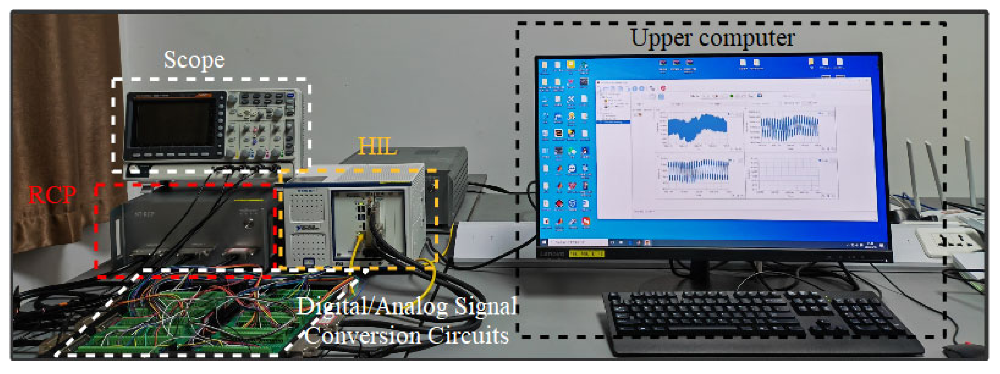
This study conducted an experimental validation of five distinct control methodologies using the StarSim Hardware-in-the-Loop (HIL) and Real-Time Control Platform (RCP), as depicted in Figure 17. The physical configuration of the experimental setup involves the transmission of the mathematical model of the photovoltaic (PV) cell to the HIL via software, alongside the uploading of the control algorithms to the RCP using similar software-based procedures. Subsequently, the RCP facilitates closed-loop control by transmitting output duty cycle signals to the HIL through dedicated signal transmission lines.

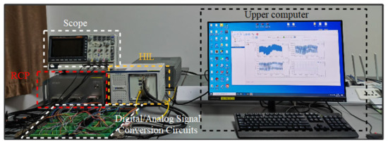
Figure 17. HIL + RCP platform.

The StarSim HIL supports the fine-grained real-time simulation of power electronics models on FPGA platforms and allows users to run customized control modules on the CPU. These control modules are versatile: they can implement closed-loop control algorithms with the power electronics models on the FPGA, as well as represent various user-defined models on the CPU, such as photovoltaic cells, wind turbines, and storage batteries. They build a fully functional real-time simulation system by combining the control modules on the CPU with the power electronics components on the FPGA.

The StarSim RCP is a software tool designed for Rapid Control Prototyping. Its configurable design allows users to easily deploy control algorithms written in Simulink or LabVIEW to NI’s real-time hardware with simple configuration and mapping operations and quickly realize the controller functions of power electronics or motor drive systems.

The StarSim RCP used version 2.1.0.1. Its target serial number is 8077-706A-A055-A14E-20DD-A092-9066-8421. There are 16 analog inputs and 4 analog outputs on the ZYNQ + 9683 (or ZYNQ + 9684), as well as an eight-way AI and eight-way AO; each FPGA board defaults to 48 digital signals, with 16 digital signals on interface 0 (Connector 0) and 32 digital signals on interface 1 (Connector 1). For the normalization of the reference wave, since the amplitude of the triangular wave is 1, it is necessary to normalize the reference wave output by the control algorithm to [−1, 1], with the normalized factor set to 0.5. It is imperative to acknowledge that the operational dynamics of the physical platform introduce harmonic distortions. To address this, the photovoltaic cell scale was expanded by utilizing two groups comprising 35 parallel-connected and 20 series-connected photovoltaic arrays. This augmentation ensured a more representative experimental environment, enhancing the results’ fidelity. Relevant parameters pertaining to the photovoltaic cells utilized in the experimentation are outlined in detail within Table 4, providing essential contextual information for the ensuing analysis and interpretation.

Table 4. Parameters of the PV cells.

Item	Value	Item	Value
Isc (A)	3.35	Radiance	500/1000
Im (A)	3.05	Series cells	35
Voc (V)	21.7	Parallel cells	20
Vm (V)	17.4	T (°C)	25

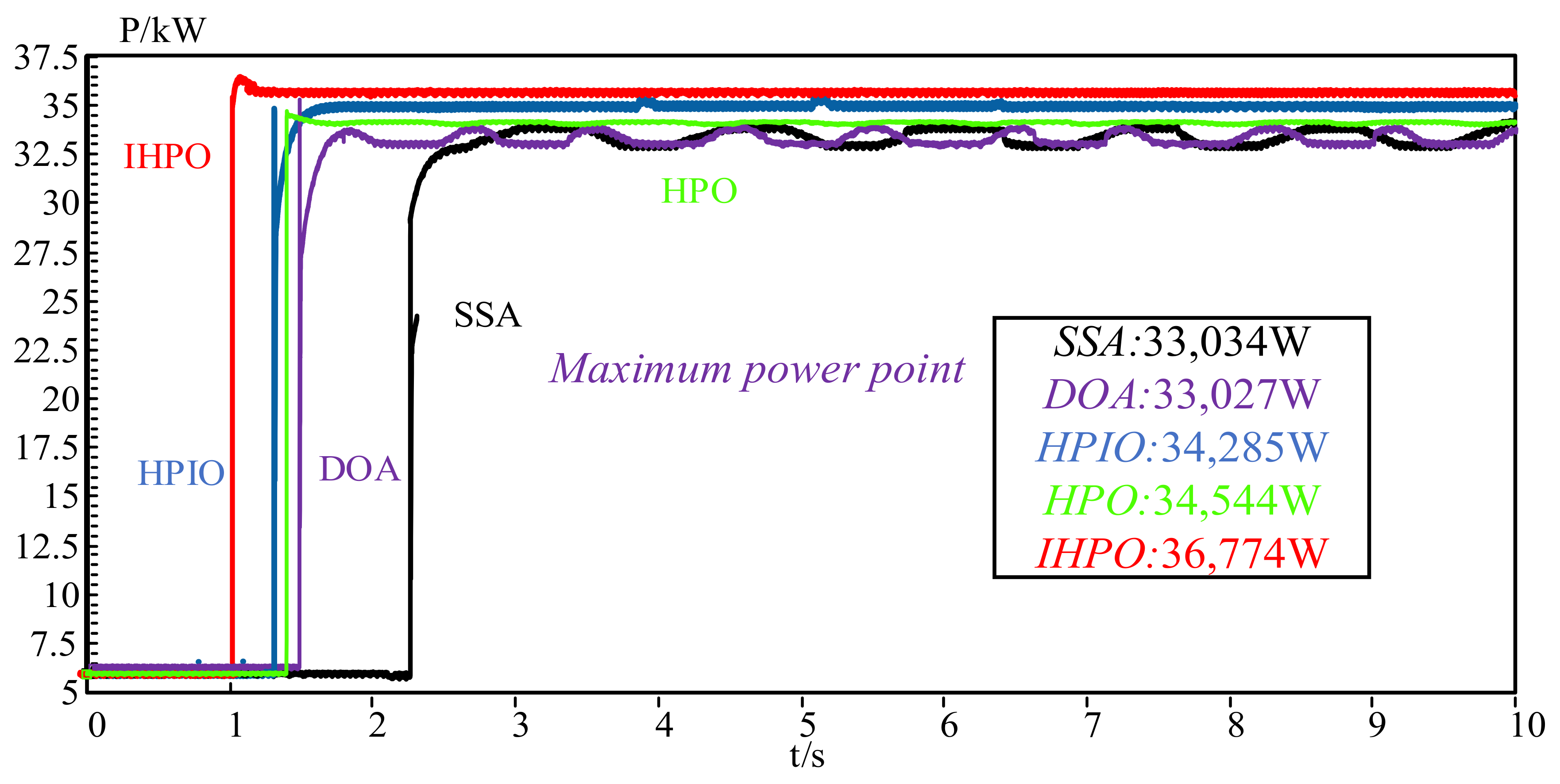
The performances of the five control methods were verified through experimental tests. As observed in Figure 18, the tracking process of the SSA and DOA control methods exhibits instability and significant fluctuations. Specifically, the average power values obtained by selecting points to average are 33,027 W for the SSA control method and 33,034 W for the DOA control method. These fluctuations may indicate a less effective tracking and energy conversion efficiency.

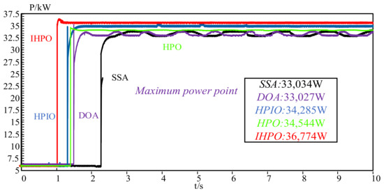
Figure 18. Power output curves for five different control methods output from the experimental platform.

In contrast, the other three control methods display smoother tracking behavior after reaching a steady state. Among them, the HPO control method achieves a final power of 34,544 W, demonstrating relatively good performance. However, the HPIO control method, while achieving rapid stability, experiences slight jitter phenomena at 4 s, 5 s, and 6 s. This may be due to the manner of the individuals in the system, where the information among the individuals may not be synchronized promptly.

To further characterize the results, additional data indicators, such as the time taken to reach the steady state, the magnitude of the fluctuations during the tracking process, and the coefficient of variation (CV) of the power output, can be useful. These indicators will provide a more comprehensive understanding of the stability, efficiency, and robustness of each control method.

In comparison, the proposed method not only achieves rapid stability but also successfully captures the maximum power point (MPP) in the power generation process. The steady-state power of the proposed method is 36,774 W, which is significantly higher than that of the other methods. This indicates that the proposed method offers superior energy conversion efficiency and stability performance.

A histogram of the output performance between the different control methods under experimental conditions is illustrated in Figure 19. It can be seen that the tracking efficiency of the SSA and DOA methods is below 90; the tracking efficiency of the HPIO and HPO control methods converges to the same level, at about 92%. The tracking efficiency of the control proposed method reaches 98.75%, which is 10.05% higher than that of the SSA control method. From the histogram of the response time (Figure 19a), it can be observed that the steady-state time of the SSA control method is 2.226 s, and the tracking time of the DOA, HPIO, and HPO methods is 1.482 s, 1.372 s, and 1.394 s, respectively. The proposed method captures the MPP within 1 s, which is 55.7% less than the SSA control method, effectively improving the immediacy of MPPT.

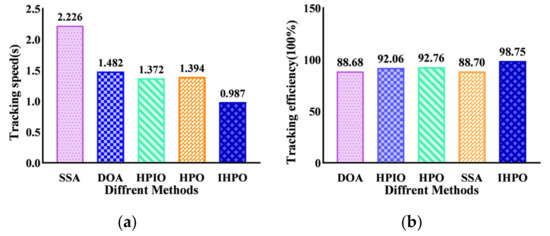
Figure 19. Tracking performances of different MPPT methods on the experimental platform: (a) tracking speed; (b) tracking efficiency.

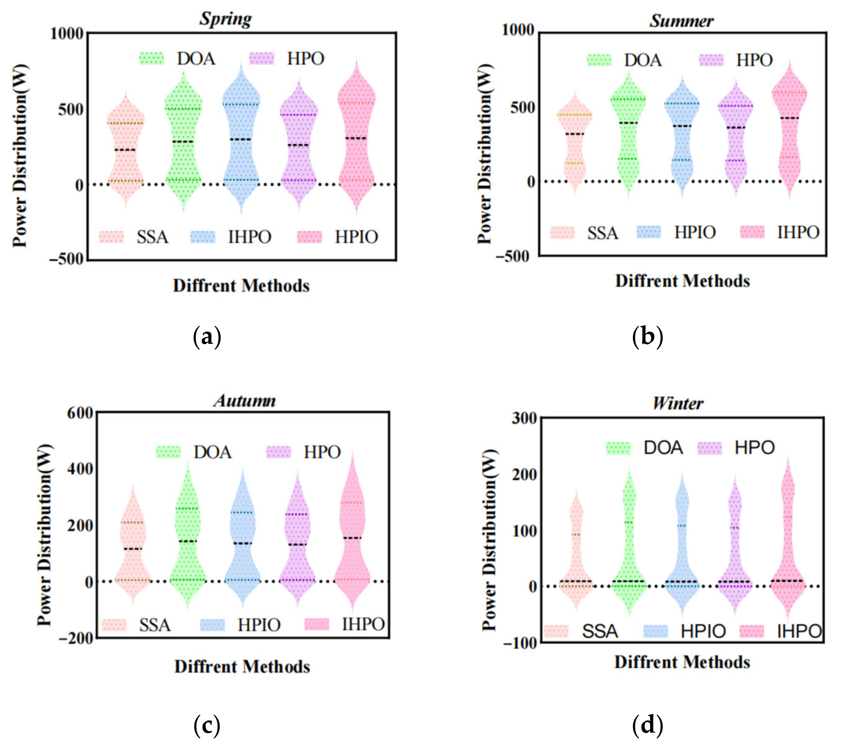
The superiority of the proposed method is further verified in this section by measuring the solar radiation of four seasonal species in Shihezi, China (longitude 68.2696 degrees; latitude 48.0207 degrees), in spring (1 April), summer (1 July), autumn (1 October), and winter (1 January). In order to better compare the power generation of the PV system throughout the year, 6:00 A.M. to 8:00 P.M. was selected as the data collection range, with a frequency of 1 h/time. Figure 20 illustrates the radiation profile. In spring, solar radiation is more regular and parabolic. The high-radiation duration is longer in summer. In contrast, autumn radiation peaks appear earlier and are primarily in a low-radiation state. In winter, the area is mostly cloudy and the radiation situation is poor, with only a stable low-radiation level between 12:00 P.M. and 15:00 P.M.

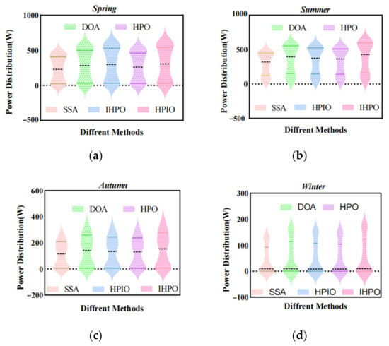
Figure 20. Output power of different control methods in four seasons: (a) spring; (b) summer; (c) autumn; (d) winter.

The output power curves of the five control methods can be obtained by importing the collected radiometric data into the test platform. Figure 20a shows that the proposed control method has the best tracking effect. The DOA tracking fails and the HPO control methods are better than the DOA method; moreover, tracking instability still exists, and the reason might be that the algorithm predation mechanism lacks dynamics. Figure 20b demonstrates that, under the premise of the radiation shape, several control methods maintain certain fluctuations, and the tracking effect of the control method proposed is closer to the ideal state. It can be seen from Figure 20c that the DOA control effect is poor, the output shape of the HPIO method is quite different from the original radiance curve, the algorithm tracking fails, and the control method proposed maintains a better tracking effect. The output power curve in winter is illustrated in Figure 20d. Considering the influence of the external environment in winter, the output of the five different control methods may be in worse performance, the control method proposed retained a good tracking effect in the SSA method, and several other control methods could not effectively capture the GMPP.

6. Conclusions

In this paper, an improved hunter–prey scheme was suggested, which improved the performance of the traditional MPPT technology to a certain extent. This method adopted a spiral search strategy to strengthen control method’s global search capability.

(1)

Compared with the existing popular population optimization methods (SSA, DOA, HPIO, and HPO), the proposed method’s response time and tracking efficiency have been significantly improved. The simulation outcome shows that the tracking efficiency of the proposed method reaches 100% under six shadow conditions, accompanied by a reduced response time. Correspondingly, good performance is achieved under dynamic shading conditions.

(2)

The output performance of the method under shading conditions is verified by embedded systems (the StarSim HIL and StarSim RCP). The experimental results illustrate that the tracking efficiency of the IHPO method reaches 98.75%.

(3)

By collecting the illumination information for four days in four seasons, the effectiveness of the method was verified in the embedded system. In practical application scenarios, the proposed method can capture the MPP.

Ultimately, the superiority of the IHPO method was verified by different experimental methods, and the experimental and simulation comparisons with the schemes in recent years were carried out to optimize the tracking process of photovoltaic power generation. In the future, the proposed IHPO control panel method can be applied to more complex photovoltaic power generation scenarios to prove its effectiveness.

References

- Korkmaz, Ö. What is the role of the rents in energy connection with economic growth for China and the United States? Resour. Policy 2022, 75, 102517. [Google Scholar] [CrossRef]
- Li, Y.; Ding, Y.; He, S. Artificial intelligence-based methods for renewable power system operation. Nat. Rev. Electr. Eng. 2024, 2, 163179. [Google Scholar] [CrossRef]
- Lin, B.; Li, Z. Towards world’s low carbon development: The role of clean energy. Appl. Energy 2022, 307, 118160. [Google Scholar] [CrossRef]
- Gutiérrez, C.; de la Vara, A.; González-Alemán, J.J.; Gaertner, M.Á. Impact of climate change on wind and photovoltaic energy resources in the canary islands and adjacent regions. Sustainability 2021, 13, 4104. [Google Scholar] [CrossRef]
- Feng, S.; Li, S.; Xu, R.; Ding, Z. Solar PV MPPT Control Technology Application Analysis. In Proceedings of the 8th International Conference on Management and Computer Science (ICMCS 2018), Shenyang, China, 10–12 August 2018; Atlantis Press: Amsterdam, The Netherlands, 2018; pp. 471–474. [Google Scholar]
- Khadidja, S.; Mountassar, M.; M’hamed, B. Comparative study of incremental conductance and perturb & observe MPPT methods for photovoltaic system. In Proceedings of the 2017 International Conference on Green Energy Conversion Systems (GECS), Hammamet, Tunisia, 23–25 March 2017; IEEE: New York, NY, USA, 2017; pp. 1–6. [Google Scholar]
- Chen, Y.; Zhou, D.; Xu, Z. Maximum power point tracking based on adaptive variable step-size incremental-resistance method. J. South China Univ. Technol. (Nat. Sci. Ed.) 2015, 43, 25–32. [Google Scholar]
- Khan, M.Y.A.; Liu, H.; Hashemzadeh, S.M.; Yuan, X. A novel high step-up DC–DC converter with improved P&O MPPT for photovoltaic applications. Electr. Power Compon. Syst. 2021, 49, 884–900. [Google Scholar]
- Chen, Y.A.; Zhou, J.H.; Li, J.; Zhou, L.L. Application of gradient variable step size MPPT algorithm in photovoltaic system. Proc. CSEE 2014, 34, 3156–3161. [Google Scholar]
- Rezazadeh, S.; Moradzadeh, A.; Pourhossein, K.; Akrami, M.; Mohammadi-Ivatloo, B.; Anvari-Moghaddam, A. Photovoltaic array reconfiguration under partial shading conditions for maximum power extraction: A state-of-the-art review and new solution method. Energy Convers. Manag. 2022, 258, 115468. [Google Scholar] [CrossRef]
- Başoğlu, M.E. An enhanced scanning-based MPPT approach for DMPPT systems. Int. J. Electron. 2018, 105, 2066–2081. [Google Scholar] [CrossRef]
- Celikel, R.; Yilmaz, M.; Gundogdu, A. A voltage scanning–based MPPT method for PV power systems under complex partial shading conditions. Renew. Energy 2022, 184, 361–373. [Google Scholar] [CrossRef]
- He, X.; He, B.; Zhao, Y.; Cui, R.; Zhang, J.; Dong, Y.; Jiang, R. MPPT control based on improved mayfly optimization algorithm under complex shading conditions. Int. J. Emerg. Electr. Power Syst. 2021, 22, 661–674. [Google Scholar] [CrossRef]
- Mao, M.; Zhang, L.; Yang, L.; Chong, B.; Huang, H.; Zhou, L. MPPT using modified salp swarm algorithm for multiple bidirectional PV-Ćuk converter system under partial shading and module mismatching. Sol. Energy 2020, 209, 334–349. [Google Scholar] [CrossRef]
- Yılmaz, M.; Corapsiz, M. Artificial Neural Network based MPPT Algorithm with Boost Converter topology for Stand-Alone PV System. Erzincan Univ. J. Sci. Technol. 2022, 15, 242–257. [Google Scholar] [CrossRef]
- Mazumdar, D.; Sain, C.; Biswas, P.K.; Sanjeevikumar, P.; Khan, B. Overview of solar photovoltaic MPPT methods: A state of the art on conventional and artificial intelligence control techniques. Int. Trans. Electr. Energy Syst. 2024, 1, 8363342. [Google Scholar] [CrossRef]
- Avila, E.; Pozo, N.; Pozo, M.; Salazar, G.; Domínguez, X. Improved particle swarm optimization based MPPT for PV systems under Partial Shading Conditions. In Proceedings of the 2017 IEEE Southern Power Electronics Conference (SPEC), Puerto Varas, Chile, 4–7 December 2017; IEEE: New York, NY, USA, 2017; pp. 1–6. [Google Scholar]
- El Hariz, Z.; Hicham, A.; Mohammed, D. A novel optimiser of MPPT by using PSO-AG and PID controller. Int. J. Ambient. Energy 2022, 43, 5199–5206. [Google Scholar] [CrossRef]
- Veeramanikandan, P.; Selvaperumal, S. Investigation of different MPPT techniques based on fuzzy logic controller for multilevel DC link inverter to solve the partial shading. Soft Comput. 2021, 25, 3143–3154. [Google Scholar] [CrossRef]
- Li, W.; Zhang, G.; Pan, T.; Zhang, Z.; Geng, Y.; Wang, J. A Lipschitz optimization-based MPPT algorithm for photovoltaic system under partial shading condition. IEEE Access 2019, 7, 126323–126333. [Google Scholar] [CrossRef]
- Sampaio, P.G.V.; González, M.O.A. Photovoltaic solar energy: Conceptual framework. Renew. Sustain. Energy Rev. 2017, 74, 590–601. [Google Scholar] [CrossRef]
- Meng, X.-L.; Liu, B.; Lopez, C.F.A.; Liu, C.-L. Multi-field coupling characteristics of photovoltaic cell under non-uniform laser beam irradiance. Sustain. Energy Technol. Assess. 2022, 52, 101963. [Google Scholar]
- Yaman, K.; Arslan, G. A detailed mathematical model and experimental validation for coupled thermal and electrical performance of a photovoltaic (PV) module. Appl. Therm. Eng. 2021, 195, 117224. [Google Scholar] [CrossRef]
- Kumar, A.; Rizwan, M.; Nangia, U.; Alaraj, M. Grey wolf optimizer-based array reconfiguration to enhance power production from solar photovoltaic plants under different scenarios. Sustainability 2021, 13, 13627. [Google Scholar] [CrossRef]
- Naruei, I.; Keynia, F.; Sabbagh Molahosseini, A. Hunter–prey optimization: Algorithm and applications. Soft Comput. 2022, 26, 1279–1314. [Google Scholar] [CrossRef]
- Fu, M.; Liu, Q. An improved Hunter–prey optimization algorithm and its application. In Proceedings of the 2022 IEEE International Conference on Networking, Sensing and Control (ICNSC), Shanghai, China, 15–18 December 2022; IEEE: New York, NY, USA, 2022; pp. 1–7. [Google Scholar]
Disclaimer/Publisher’s Note: The statements, opinions and data contained in all publications are solely those of the individual author(s) and contributor(s) and not of MDPI and/or the editor(s). MDPI and/or the editor(s) disclaim responsibility for any injury to people or property resulting from any ideas, methods, instructions or products referred to in the content. |
© 2024 by the authors. Licensee MDPI, Basel, Switzerland. This article is an open access article distributed under the terms and conditions of the Creative Commons Attribution (CC BY) license (https://creativecommons.org/licenses/by/4.0/).