Content-Adaptive Bitrate Ladder Estimation in High-Efficiency Video Coding Utilizing Spatiotemporal Resolutions

Abstract

The constant increase in multimedia Internet traffic in the form of video streaming requires new solutions for efficient video coding to save bandwidth and network resources. HTTP adaptive streaming (HAS), the most widely used solution for video streaming, allows the client to adaptively select the bitrate according to the transmission conditions. For this purpose, multiple presentations of the same video content are generated on the video server, which contains video sequences encoded at different bitrates with resolution adjustment to achieve the best Quality of Experience (QoE). This set of bitrate–resolution pairs is called a bitrate ladder. In addition to the traditional one-size-fits-all scheme for the bitrate ladder, context-aware solutions have recently been proposed that enable optimum bitrate–resolution pairs for video sequences of different complexity. However, these solutions use only spatial resolution for optimization, while the selection of the optimal combination of spatial and temporal resolution for a given bitrate has not been sufficiently investigated. This paper proposes bit-ladder optimization considering spatiotemporal features of video sequences and usage of optimal spatial and temporal resolution related to video content complexity. Optimization along two dimensions of resolution significantly increases the complexity of the problem and the approach of intensive encoding for all spatial and temporal resolutions in a wide range of bitrates, for each video sequence, is not feasible in real time. In order to reduce the level of complexity, we propose a data augmentation using a neural network (NN)-based model. To train the NN model, we used seven video sequences of different content complexity, encoded with the HEVC encoder at five different spatial resolutions (SR) up to 4K. Also, all video sequences were encoded using four frame rates up to 120 fps, presenting different temporal resolutions (TR). The Structural Similarity Index Measure (SSIM) is used as an objective video quality metric. After data augmentation, we propose NN models that estimate optimal TR and bitrate values as switching points to a higher SR. These results can be further used as input parameters for the bitrate ladder construction for video sequences of a certain complexity.

1. Introduction

The rapid increase in multimedia Internet traffic, especially in video streaming, requires new and more efficient solutions for video coding to improve the management of bandwidth and network resources. The quality of content delivered to clients can vary due to factors like network bandwidth, viewing conditions, and display specifications. To maximize visual quality while minimizing bitrate, streaming providers utilize advanced video streaming technologies and standards, including HTTP adaptive streaming (HAS) [1]. HAS has become the most widely used method for video streaming, allowing viewers to experience smoother playback by automatically adjusting the bitrate of video sequences based on current network conditions. This is achieved by creating multiple versions of the same video, each encoded using different parameters known as a bitrate ladder. Adaptive video streaming requires the definition of multiple parameters, including combinations of spatial resolution, bitrate, and temporal resolution (i.e., frame rate). Each configuration results in different throughput requirements, allowing for efficient streaming across varying network conditions [2]. After encoding, video sequences are divided into smaller segments with a duration ranging from two to ten seconds and stored on the server side of such systems. This ensures that clients receive the best possible Quality of Experience (QoE) depending on their display capabilities and network conditions [3]. HTTP live streaming (HLS), introduced by Apple [4], and dynamic adaptive streaming over HTTP (DASH), developed by MPEG [5], are types of streaming architectures that both require a bitrate ladder for video streaming. Traditionally, bitrate ladders that consist of spatial resolution (SR)–bitrate pairs have been constructed using a ‘one-size-fits-all’ approach, which does not consider the varying complexities of different video sequences. While the ‘one-size-fits-all’ approach is optimized for general video characteristics, it does not ensure an optimal bitrate ladder for every video sequence. Achieving the best possible quality requires a more tailored approach [6]. Recently, more advanced, context-aware methods have been developed to optimize these bitrate–resolution pairs based on the specific complexity of each video. However, these methods have primarily focused on optimizing spatial resolution, without fully exploring how combining both spatial and temporal resolutions could improve video quality and streaming efficiency. Recent advancements in devices capable of recording and displaying video sequences with 4K and 8K spatial resolutions, as well as temporal resolutions up to 120 frames per second (fps), have significantly enhanced visual sharpness [7]. These developments have also contributed to the reduction in temporal artifacts such as motion blur, flickering, and stuttering [8]. Several studies have examined the impact of reduced temporal resolution on Quality of Experience (QoE) [9], particularly in relation to issues such as jitter and jerkiness [10]. In cases when network conditions required the use of lower bitrates, the QoE was found to be higher when video sequences were encoded using lower SR compared to video sequences with lower temporal resolution (TR) [11]. Based on the analysis of QCIF and CIF sequences, at 7.5, 15, and 30 fps, encoded with H.263 and H.264 encoders, the authors in [11] determined that the optimal combination of spatial and temporal resolution that ensures the best perceptual quality for a given bitrate varies depending on the spatiotemporal complexity of the sequence. Also, when streaming video sequences with more temporal information (TI) [12], perceptual quality was found to be higher when such video sequences were encoded using lower TR [11]. This being said, TR is rarely taken into consideration in the relevant literature and thus should be investigated more thoroughly.

This paper introduces a novel approach to bitrate ladder optimization that considers both the spatial and temporal resolutions, up to 4k and 120 fps, respectively. Bitrate ladder optimization is described as the process of refining model performance to achieve better selection of bitrate ladders. By selecting an optimal combination of spatial and temporal resolutions tailored to the complexity of the video content, our method aims to enhance streaming efficiency and the overall viewing experience. Given the added complexity of optimizing two dimensions, traditional methods that involve intensive encoding for all possible resolutions and bitrates are not practical for real-time applications. To address this, we propose using a neural network (NN)-based model for data augmentation, which simplifies the process. The model is trained on a set of video sequences with varying levels of complexity, encoded at different spatial and temporal resolutions using the High-Efficiency Video Coding (HEVC) standard. We use the Structural Similarity Index Measure (SSIM) to objectively assess video quality. The SSIM is employed as the video quality assessment metric, selected due to its superior performance compared to other metrics used for assessing the quality of video sequences in streaming environments [13]. After data augmentation, two NN models are then used to estimate optimal temporal resolution and bitrate pairs as switching points to higher spatial resolutions, providing a starting point for building more efficient bitrate ladders. Our results show that this approach simplifies the construction of the bitrate ladder and offers a practical solution for real-time streaming. By incorporating spatiotemporal optimization, this method represents a significant step forward in adaptive streaming technology, improving the efficiency and quality of video streaming in a wide range of network environments. To facilitate the reproducibility of our results, we will publish a database containing the encoded video sequences, augmented data, and NN models. This resource will serve as a foundation for future research involving video sequences with temporal resolutions of up to 120 fps.

The structure of this paper is as follows: Following the introduction, Section 2 provides an overview of related work, focusing on the application of AI technologies, including machine learning (ML) and NNs, in constructing optimal bitrate ladders for video streaming. Section 3 details the experimental setup, describes the video sequence precoding process, and provides an in-depth overview of the published database, along with the flowchart outlining the model development process. The subsequent section, preceding the conclusion, offers a comprehensive analysis of the developed models and the corresponding test results.

2. Related Work

The traditional use of a fixed bitrate ladder for video sequences with content of different complexity is not optimal for video streaming applications [3]. By recognizing this limitation, various methods have been proposed to redefine bitrate ladders for different contents. For instance, Netflix introduced a per-title encoding optimization approach, where bitrate ladders are content dependent. Initially, Netflix’s per-title method involved encoding the entire video at a different BR and SR to construct the convex hull of rate–distortion (RD) curves using Video Multimethod Assessment Fusion (VMAF) as an objective video quality metric [14]. However, this method was found to be suboptimal, as a video can consist of scenes with varying visual complexities. To address this, Netflix proposed a novel solution that, before coding, first involves dividing the video into large video segments that have similar adjacent frames that respond similarly to changes in encoding parameters [15]. Per-title encoding schemes design a convex hull that is determined for every video sequence, which consists of optimal SR–bitrate pairs that display the highest QoE at the desired bitrate. This convex hull, where the encoding point achieves Pareto efficiency, is crucial for optimizing the viewing experience. However, a significant drawback of this approach is its requirement for extensive computational resources and time. Specifically, for a set of SR and bitrates (BRs), constructing a convex hull necessitates compressing the video SR × BR times, followed by selecting the optimal SR for a certain BR [6].

Recent advancements in video streaming technologies have led to the development of more sophisticated methods for optimizing bitrate ladders, which are essential for ensuring high-quality video delivery under varying network conditions. The idea behind the following work was to eliminate the need for exhaustive encoding for constructing convex hulls for video sequences with different content complexity. Researchers have advanced the modeling of rate–distortion curves by employing polynomial representations and leveraging video texture features to predict polynomial coefficients using ML Support Vector Regression models [16,17]. This established a correlation between video texture characteristics and RD curves, enhancing the accuracy of bitrate ladder predictions. Building on this foundation, subsequent research presented in [18,19] extended the approach by modeling key points on the convex hull, using similar video texture features to predict crossover quantization parameters between rate–quality (RQ) curves at different resolutions. Moreover, a study presented in [20] explored the use of linear regression models in modeling VMAF as a function of DCT-based energy features and bitrate, demonstrating a high correlation with VMAF. Another solution that uses ML, but mitigates the need for additional computational steps for feature extraction, integrates a full-reference quality estimation model directly into the video-delivery pipeline [6]. The authors used ML models based on Extra-Trees, XG-Boost, and Random Forest for parameter estimation for video sequences with a TR of 60 fps and a bit depth of 10 bits per sample. ML models (Support Vector Machines with different kernels, Random Forests, and Gaussian Processes) are also used in [21], where the authors estimate the bitrate ladder while taking into account the content complexity by evaluating spatiotemporal features of video sequences. The SR-BR pairs that represent switching points to a higher SR are determined based on RQ curves constructed using VMAF as an objective video metric. The authors developed their model by encoding video sequences with 4k SR and 60 fps TR. As a continuation of previous work, the authors in [19] used ML technologies for content-optimized bitrate ladder estimation for application in on-demand video services. As in previous research, Support Vector Machines with different kernels and Random Forests were used to develop models based on results acquired by encoding video sequences that have TR of 60 fps. Both presented methods achieve the reduction in the number of encodes needed per video sequence. A content-agnostic method designed to predict the crossover points associated with RQ curves, facilitating a content-customized estimation of the bitrate ladder, is also presented in [18]. This approach involves extracting spatiotemporal features from video sequences with 60 fps and, by leveraging ML techniques, the method predicts SR-BR pairs that represent switching points to a higher SR. Research that also considers deep learning (DL) apart from ML is presented in [22]. This research also considers only video sequences that have a TR of 60 fps. In order to train a convolutional neural network from scratch, the authors needed a large amount of data; thus, they used pre-trained models on ImageNet [23] to serve as deep feature descriptors.

Apart from solutions from Netflix, there are other per-title encoding methods that were developed by the industry like Bitmovin [24] and CAMBRIA [25] which calculate the encoding complexity. In [24], a complexity analysis is conducted on all input video sequences, generating a range of measurements that are processed by an ML model to estimate dynamically a content-agnostic bitrate ladder. In [25], complexity is estimated by implementing a fast constant rate factor encoding. Although the aforementioned solutions present significant advancements, their proprietary nature limits the availability of detailed information and precludes direct comparisons. Additionally, many of these approaches depend on extensive encoding processes, leading to substantial computational, energy, and financial costs [26].

Deep learning models have also been utilized to estimate convex hull points and thereby predict the bitrate ladder by approaching the problem as a multi-label classification task [27]. MUX [28] was introduced by the industry as a proprietary solution that comprises a multi-layer NN approach that inputs vectorized video frames to estimate the bitrate ladder. The application of Deep Neural Networks (DNNs) to bitrate ladder prediction has not yet been extensively explored due to the fact that they typically need large training datasets to achieve generalization, which can be resource intensive and expensive [23]. To mitigate this challenge, research presented in [29] repurposes the feature maps from a pre-trained network in order to predict needed parameters that are distinct from those the network was originally trained on [29]. In this context, the authors in [30] integrated pre-trained DNN modules to extract spatiotemporal features. Through transfer learning, these pre-trained models are used for bitrate ladder construction, specifically to predict SR-BR pairs that represent switching points to a higher SR. Video sequences used in this research have also the maximal TR of 60 fps and Full HD SR.

In contrast to the previously discussed studies, the only research that incorporates TR as a parameter is presented in [31]. In this work, the authors estimate the convex hull for each video sequence, utilizing both PSNR and VMAF as objective metrics. However, their approach does not employ ML or DL techniques for bitrate ladder estimation, which results in a higher demand for computational resources. The modeling was conducted using video sequences with an SR up to Full HD and a TR up to 120 fps. The findings demonstrate that the proposed method enhances bitrate efficiency by taking TR into account alongside SR, but does not provide any method for prediction of an optimal SR-TR-BR combination for some new video content.

Compared to previous work, our approach employs NN models capable of estimating switching points to a higher SR, i.e., optimal values of TR-SR-BR combinations necessary for the construction of bitrate ladders for video sequences with high temporal resolutions, up to 120 fps, and spatial resolutions of 4K. By leveraging these advanced models, our method not only enhances the accuracy of bitrate ladder predictions but also reduces the computational demands typically associated with such processes. Experimental results demonstrate that our method significantly improves bitrate savings while maintaining high visual quality, making it a viable solution for adaptive video streaming. Considering the lack of large datasets that can be used for constructing NN models in the relevant literature, we also propose a novel dataset with augmented data that can be used for such purposes.

3. Database Development

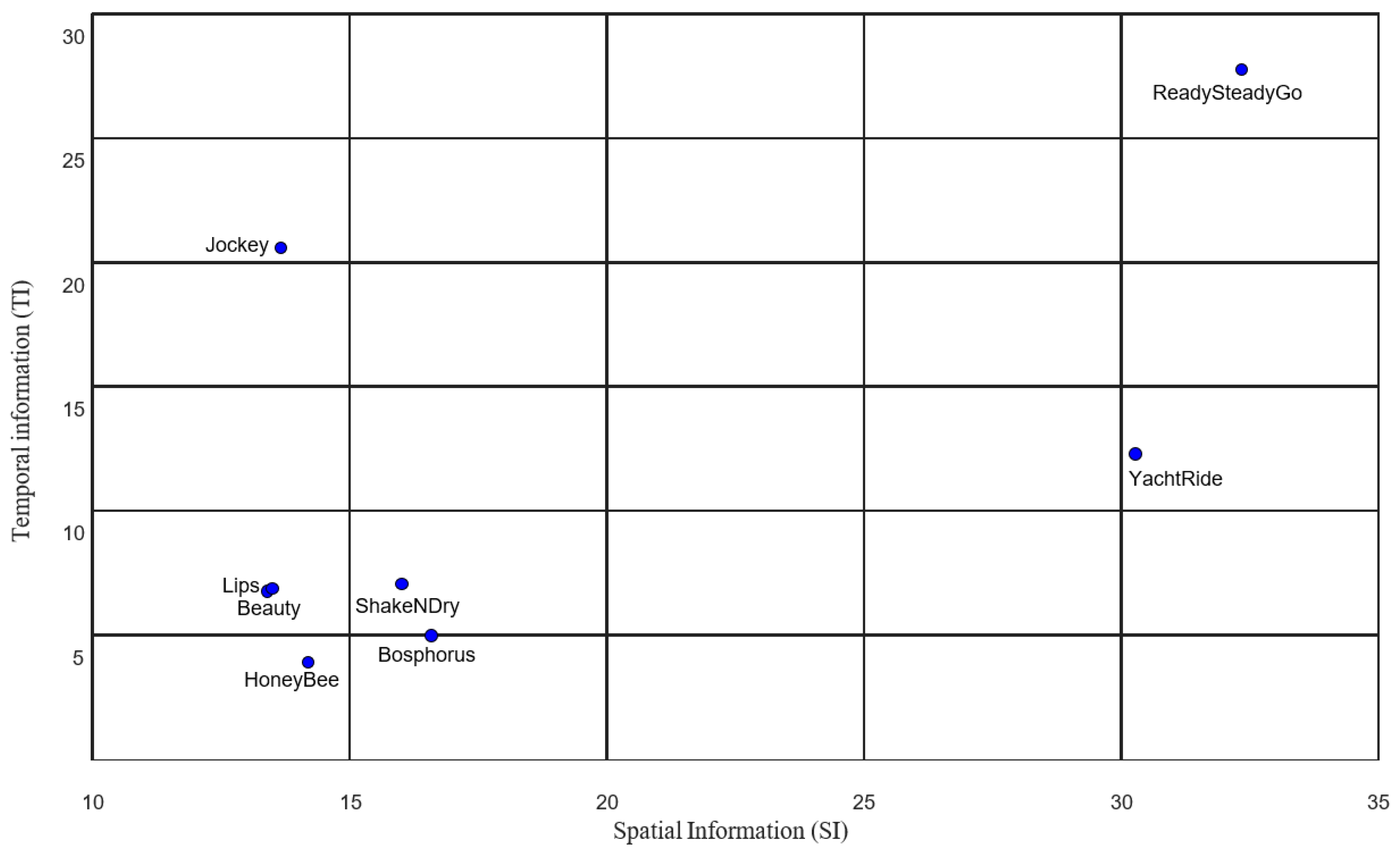
The construction of the database is a preliminary step in model development, particularly because the necessary data for 4K and 120 fps resolutions—resolutions that are increasingly common in video streaming—are currently unavailable. Therefore, this phase is crucial to ensure that the model is trained with the appropriate datasets, especially for high-resolution content where research and available data are still limited. To construct a comprehensive database of video signals, uncompressed video sequences were sourced from the Ultra Video Group repository [32]. For this study, eight video sequences—YachtRide, Bosphorus, ReadySteadyGo, HoneyBey, Jockey, ShakeNDry, Beauty, and Lips—were selected to represent varying degrees of spatial and temporal complexity. The selection of these sequences was based on their distinct spatial and temporal characteristics, quantified using the Spatial Information (SI) and TI metrics, respectively. SI and TI for the video sequences were calculated based on the Y color component of the original YUV format videos. The SI metric represents the degree of spatial variation in a video frame and is computed using the variance of pixel intensities. The TI metric measures motion between successive frames using frame differences. SI and TI are computed as time averages using equations that are defined in ITU-T P.910 (10/2023) guidelines [12]. The SI and TI values for the chosen sequences are presented in Figure 1.

Figure 1. Spatial and temporal information of video sequences used for model development and evaluation.

All video sequences were acquired at a 4K spatial resolution (3840 × 2160) and a temporal resolution of 120 fps, with an 8-bit depth per pixel in YUV format. These sequences were then encoded using an open-source program called Ffmpeg [33] at various bitrates and across different spatial and temporal resolutions. Additionally, they served as reference sequences for evaluating the quality of the encoded outputs using the SSIM objective video quality metric. The parameters varied during the study included spatial resolution and bitrate, as detailed in Table 1. The temporal resolutions used in this study are 120 fps, 60 fps, 30 fps, and 25 fps.

Table 1. Spatial resolutions and bitrates used in this study.

Spatial Resolution	480 × 360	1280 × 720	1920 × 1080	3840 × 2160
Bitrate [kbps]	50	50	250	700
	250	250	700	2400
	500 700	700 2400	2400 6200	6200 10,000

Before adjusting the temporal resolution and bitrate parameters, it was necessary to downscale the original video sequences to the desired spatial resolutions for subsequent encodings. This process is exemplified using the Beauty sequence. The original video file, Beauty_3840×2160.yuv, was downscaled to resolutions of 1920 × 1080, 1280 × 720, and 480 × 360 using the ffmpeg video scaling command. For instance, to scale the resolution to 1920 × 1080, the following command was used:

• ffmpeg -s:v 3840:2160 -i Beauty_3840×2160.yuv -vf scale=1920:1080 Beauty_1920×1080.yuv

In this command, “ffmpeg” initiates the video processing tool via the operating system’s console. The flag “-s:v 3840:2160” specifies the original resolution of the video, ensuring it matches the input file. The “-i Beauty_3840×2160.yuv” parameter designates the input video file, while “-vf scale=1920:1080” resizes the video to the target resolution of 1920 × 1080. The final output is saved as “Beauty_1920×1080.yuv”. Following the spatial resolution scaling, it is essential to adjust the temporal resolution of the video sequences. Each spatial resolution is scaled from the original 120 fps to 60, 30, and 25 fps. Temporal resolution scaling is accomplished using the following command:

• ffmpeg -s:v 3840×2160 -itsscale 0.5 -i Beauty_3840×2160.yuv Beauty_3840x2160_60fps.yuv

In this command, the “-itsscale” parameter adjusts the timestamps of the input file to ensure that the output video sequence maintains the same duration as the original, despite the change in temporal resolution. The “scale” coefficient specified with the “-itsscale” command determines the output sequence’s temporal resolution. For a temporal resolution of 60 fps, the scale parameter is set to 0.5; for 30 fps, it is set to 0.25; and for 25 fps, it is set to 0.2083. The subsequent step involves encoding the sequences at all temporal and spatial resolutions with varying bitrates. Encoding is performed using the following command:

• ffmpeg -s:v 3840×2160 -r 120 -i Beauty_3840×2160.yuv -b:v 700k -c:v libx265 Beauty_3840_700kb_120fps.265

In this command, “-r 120” specifies that the video sequence should be encoded at a temporal resolution of 120 fps. The “-b:v 700k” flag sets the bitrate to 700 kb/s, while “-c:v libx265” instructs the use of the H.265 encoder for encoding the video sequence. Additionally, the spatial resolutions of all encoded video sequences are then upscaled back to the original 3840 × 2160 resolution using the following command:

• ffmpeg -i Beauty_3840_10000kb_120fps.265 -vf scale=3840:2160:flags=bilinear Beauty_3840_10000kb_120fps_bilin.265

Here, the flag “bilinear” is included in the spatial scaling command to apply bilinear interpolation, which is used to calculate the position of each new pixel based on the positions of the four surrounding reference pixels, thereby achieving the desired spatial resolution change. The final step involves restoring the temporal resolution of the video sequence to its original 120 fps using an appropriate ffmpeg that utilizes motion interpolation to adjust the temporal resolution of a video sequence:

• ffmpeg.exe -i “Beauty_3840_10000kb_120fps_bilin.265” -filter:v “minterpolate=‘fps=120:mi_mode=mci:mc_mode=aobmc:me_mode=bidir:me=epzs’“ “Beauty_3840_10000kb_120fps_bilin_mint.265”

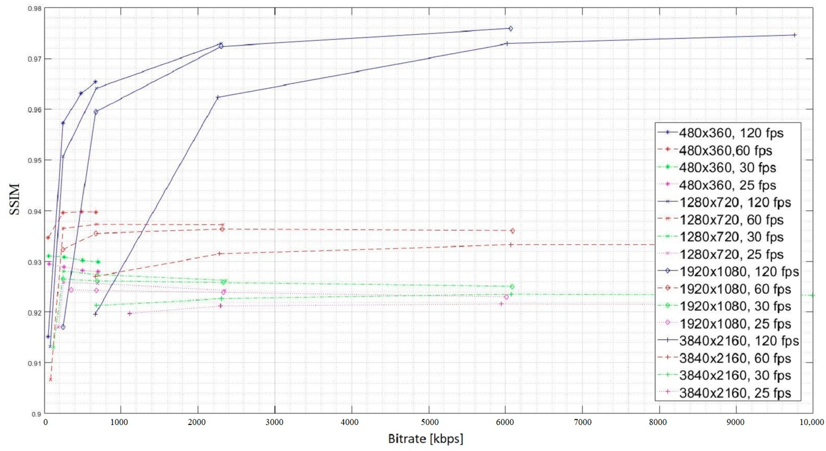
This command leverages the temporal redundancy between frames to enhance the time resolution through motion interpolation. The process typically employs the Full Search Block Matching Algorithm, which conducts motion estimation on a pixel-by-pixel basis. The parameter “fps = 120” specifies the desired temporal resolution of the output video, setting it to 120 frames per second. The “mi_mode=mci” option configures the motion interpolation mode to Motion Compensated Interpolation, enabling the “mc_mode=aobmc” parameter, which indicates the use of Adaptive Overlapping Block Motion Compensation. The “me_mode=bidir” setting applies bidirectional motion estimation, estimating displacement vectors from both forward and backward directions. The “me=epzs” parameter designates the Enhanced Predictive Zonal Search algorithm as the motion estimation method. All other motion interpolation parameters are set to their default values. To evaluate the quality of the encoded video sequences, the SSIM objective video quality metric is employed. SSIM values are computed by comparing the encoded sequences—across different spatial and temporal resolutions—against the original video sequence (4K, 120 fps) encoded at a bitrate of 30,000 kbit/s. The SSIM was also used in order to take into consideration the noise that can be introduced during the video capture or encoding process, and the SSIM is highly sensitive to noise and visual distortions. The resultant values for the video sequence Beauty are given in Figure 2. The aforementioned process was repeated for all eight video sequences.

Figure 2. Achieved bitrate quality curves for video sequence Beauty.

4. Models for BR, TR, and SSIM Estimation

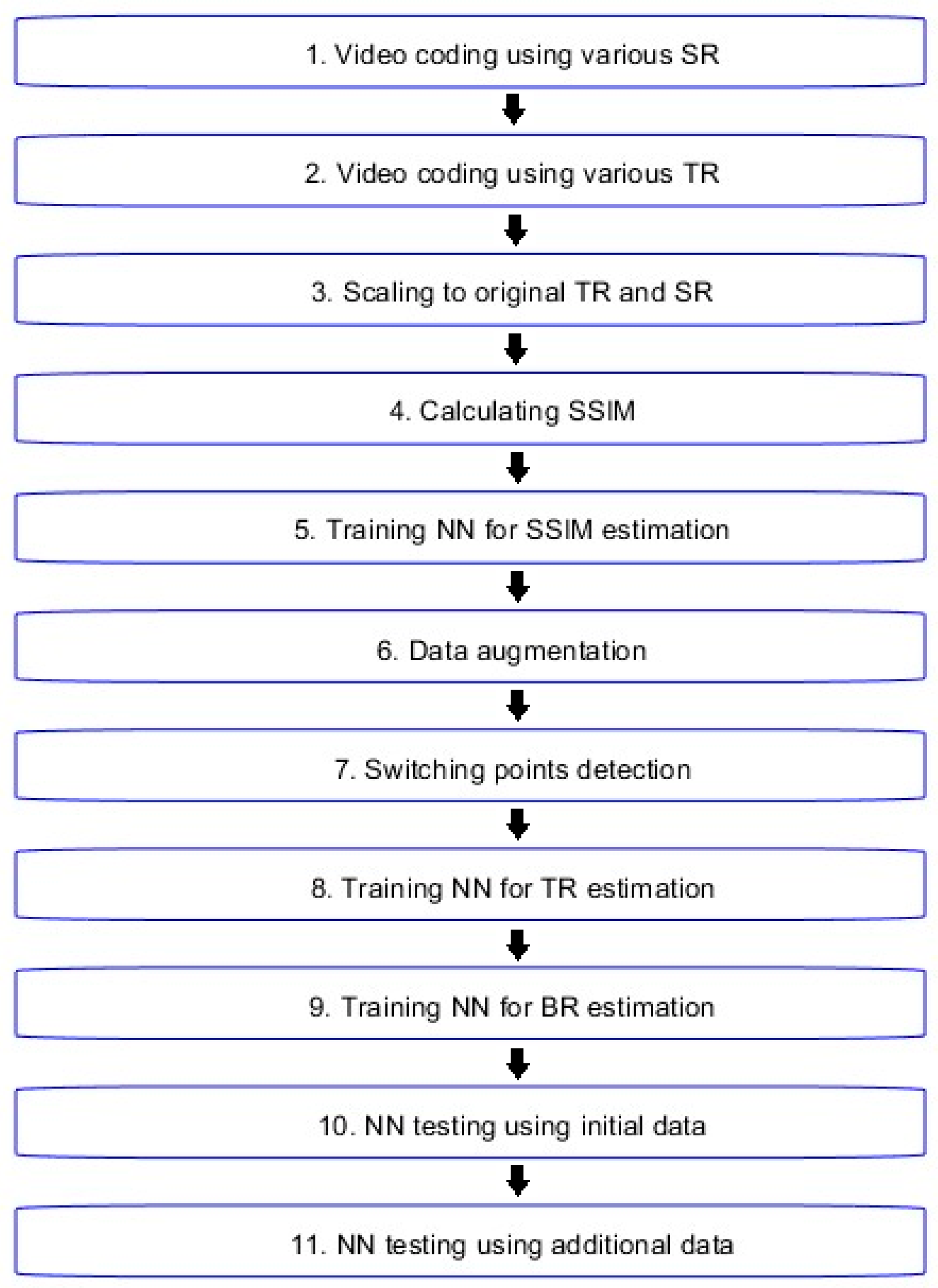
Building upon the previous section, the next phase focuses on developing a predictive model capable of effectively estimating video bitrate through neural networks, leveraging spatiotemporal characteristics for improved performance across different resolutions. To better explain the following process, a flowchart, depicted in Figure 3, was constructed. The flowchart outlines a systematic process for video coding and NN training aimed at optimizing video quality and bitrate ladder estimation. As stated earlier, the process began with video coding using various SRs and TRs. Following the initial encoding steps, the video sequences were scaled back to their original temporal and spatial resolutions. The SSIM was finally calculated to assess the quality of the encoded video sequences. After video coding and gathering initial data, which are published together with the database that includes all video sequences encoded for this study, the modeling process started by training the NN that can estimate SSIM values while using SI, TI, TR, SR, and BR as input values. NN training was followed by data augmentation to enhance the training dataset. Data augmentation was performed in order to minimize the effect of a smaller range of SI and TI in the initial dataset that may cause a narrower distribution of data, potentially introducing some bias in the model’s training. This augmentation process increased the diversity of the dataset, allowing the model to generalize better across a broader range of spatial and temporal complexities. The dataset that consists of switching points to a higher SR was then constructed based on the augmented dataset using a MATLAB script which was crucial for determining optimal transitions for TR and bitrate. Subsequently, additional neural networks were trained using the dataset that consists of switching points, one for estimating optimal TR and another for estimating optimal BR as parameters of the optimal switching point to a higher SR. Finally, the trained neural networks were tested using both the initial and the additional datasets, ensuring their robustness and accuracy in predicting video quality and encoding parameters.

Figure 3. Flowchart of video coding and NN training process.

For the training of the first NN, seven out of eight video sequences were used, and the video sequence Lips was only used for additional testing. This comprehensive workflow integrates video processing with advanced machine learning techniques to achieve optimal video streaming performance. The steps outlined in the flowchart will be explained in detail in the following sections.

4.1. Data Augmentation Process

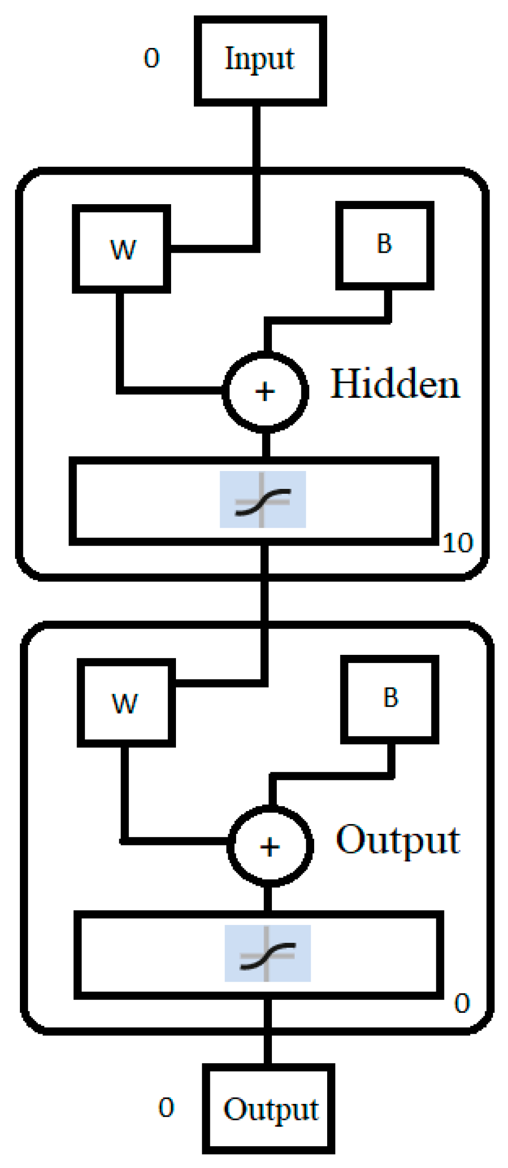
Following the video coding process and the collection of initial data, the modeling phase commenced. This phase began with training an NN capable of estimating SSIM values, using SI, TI, TR, SR, and BR as input parameters. From the acquired data, 70% of the initial data were used as training data, 15% were used as validation data, and 15% were used as test data. The data that consisted of 448 × 5 predictor data and 448 response data were divided randomly. The Levenberg–Marquardt algorithm in MATLAB R2023b with ten layers was used for training a two-layer feedforward network with sigmoid hidden neurons and linear output neurons (suitable for regression tasks). The first layer, or hidden layer, consists of neurons with a log-sigmoid activation function, which introduces nonlinearity, allowing the network to learn complex, nonlinear relationships between the input and output vectors. The second layer, or output layer, employs a linear activation function, which is typical for function fitting or nonlinear regression problems, as it ensures that the network can produce continuous output values. This architecture enables the approximation of any function with a finite number of discontinuities, provided there are sufficient neurons in the hidden layer. The use of nonlinear activation in the hidden layer combined with a linear output layer ensures that the network can generalize effectively, making it suitable for applications such as video quality prediction and bitrate ladder estimation. During the training phase, the Mean Squared Error (MSE) was used as the loss function, which is a common choice for regression tasks where the goal is to minimize the difference between predicted and actual values. The underlying NN architecture is given in Figure 4. The training progress is presented in Table 2.

Figure 4. The underlying NN architecture.

Table 2. NN training progress data.

Unit	Initial Value	Stop Value	Target Value
Epoch	0	17	1000
Performance (MSE)	305	1.2	0
Gradient	469	0.384	1 × 10−7
Mu	0.001	0.01	1 × 1010
Validation checks	0	6	6

The NN training process demonstrated strong performance, with significant improvements across key metrics, although the training was halted at epoch 17, well before the intended 1000 epochs. This early stop was due to the validation checks reaching their threshold, a safeguard to prevent overfitting and ensure the model generalizes well. Training proceeded until the stopping criterion was satisfied, specifically, when the validation error exceeded the minimum validation error achieved in the previous iterations for six consecutive validation steps. The performance metric, i.e., the MSE, saw a substantial reduction from 305 to 1.2, indicating that the model was effectively learning and nearing optimal performance, even if it did not reach the absolute target of 0. Similarly, the gradient value decreased from 469 to 0.384, showing that the model was successfully converging, though it had not yet fully minimized the loss function to the very low target value.

The Mu parameter, which controls adjustments in the optimization process, increased slightly from 0.001 to 0.01, indicating stable and appropriate step sizes throughout the training. The validation checks reached their limit at 6, prompting the early stopping mechanism, which suggests that the model was performing well and that further training might have risked overfitting. During testing, the average inference time per sample was 0.0284 s, which comfortably meets the requirements for real-time video streaming. Overall, the NN demonstrated satisfactory learning behavior, with early stopping balancing the need for performance against the risk of overfitting, though there remains room for improvement.

The training results can be seen in Table 3. The results from the NN training and testing phases indicate strong performance across the majority of the datasets, with some variability observed in the additional test set. During the training phase, the model achieved an MSE of 1.3763 and a correlation coefficient (R) of 0.9097, reflecting a high degree of accuracy and a strong relationship between the predicted and actual values. The validation phase further confirmed the model’s effectiveness, with a slightly lower MSE of 1.2566 and an improved R value of 0.9363, indicating that the model was well tuned and capable of generalizing to new data. In the test phase, the model maintained consistent performance, achieving an MSE of 1.3538 and an R value of 0.8989, demonstrating that the model’s predictions remained accurate when applied to a separate test dataset. However, the additional test set presented a more challenging scenario, with a notably higher MSE of 22.8856 and a reduced R value of 0.7913. This suggests that the additional test set may have included more complex or diverse data, which the model found more difficult to predict accurately.

Table 3. NN training results.

	Observations	MSE	R
Training	314	1.3763	0.9097
Validation	67	1.2566	0.9363
Test	67	1.3538	0.8989
Additional test	64	22.8856	0.7913

Overall, the NN exhibited strong performance during training, validation, and the initial test phase, with a slight decrease in performance on the additional test set. This could indicate areas for further refinement, particularly in enhancing the model’s ability to handle a broader range of data scenarios. Despite this, the high R values across the board indicate that the model generally performs well and maintains a strong predictive capability.

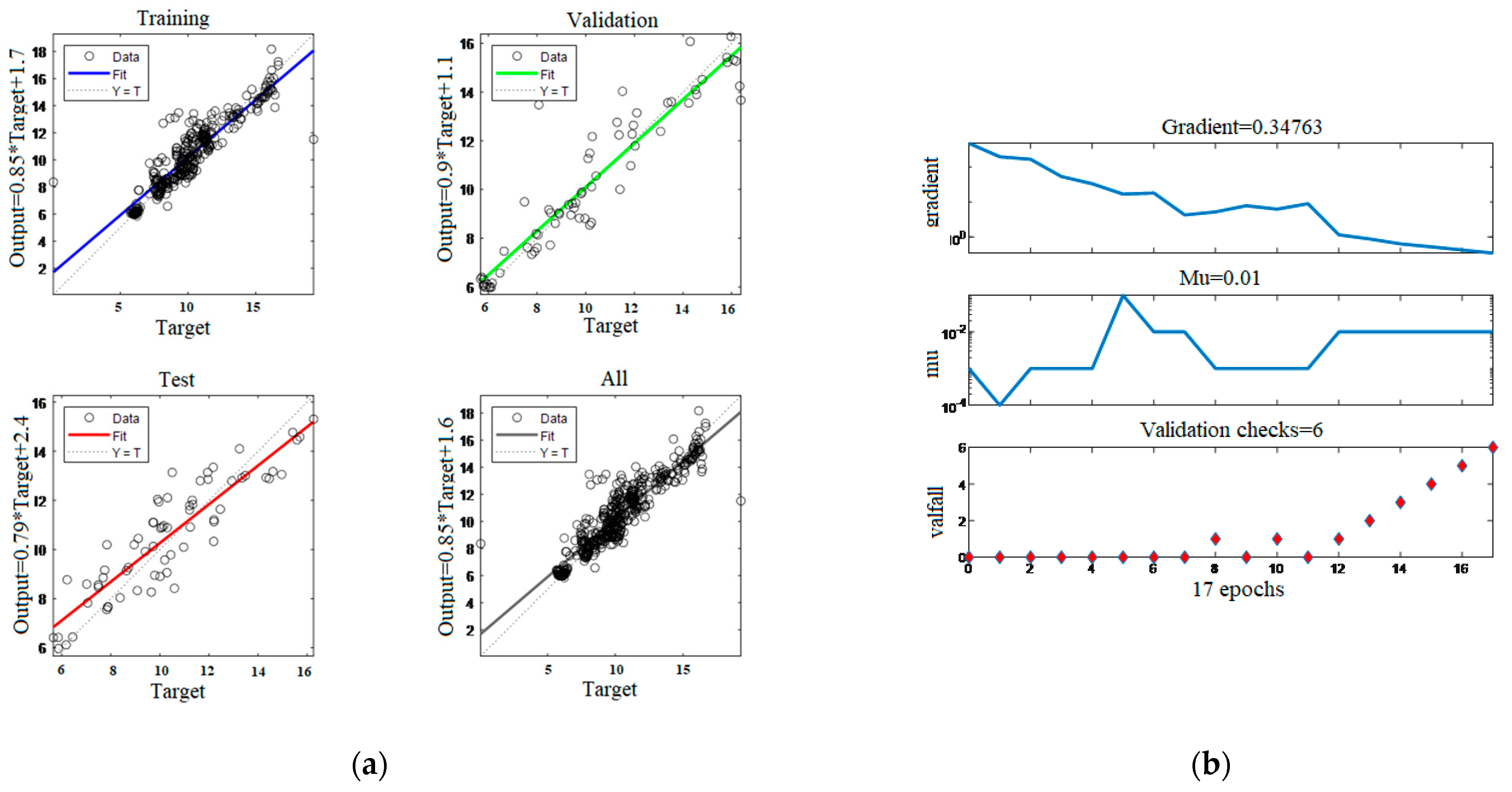
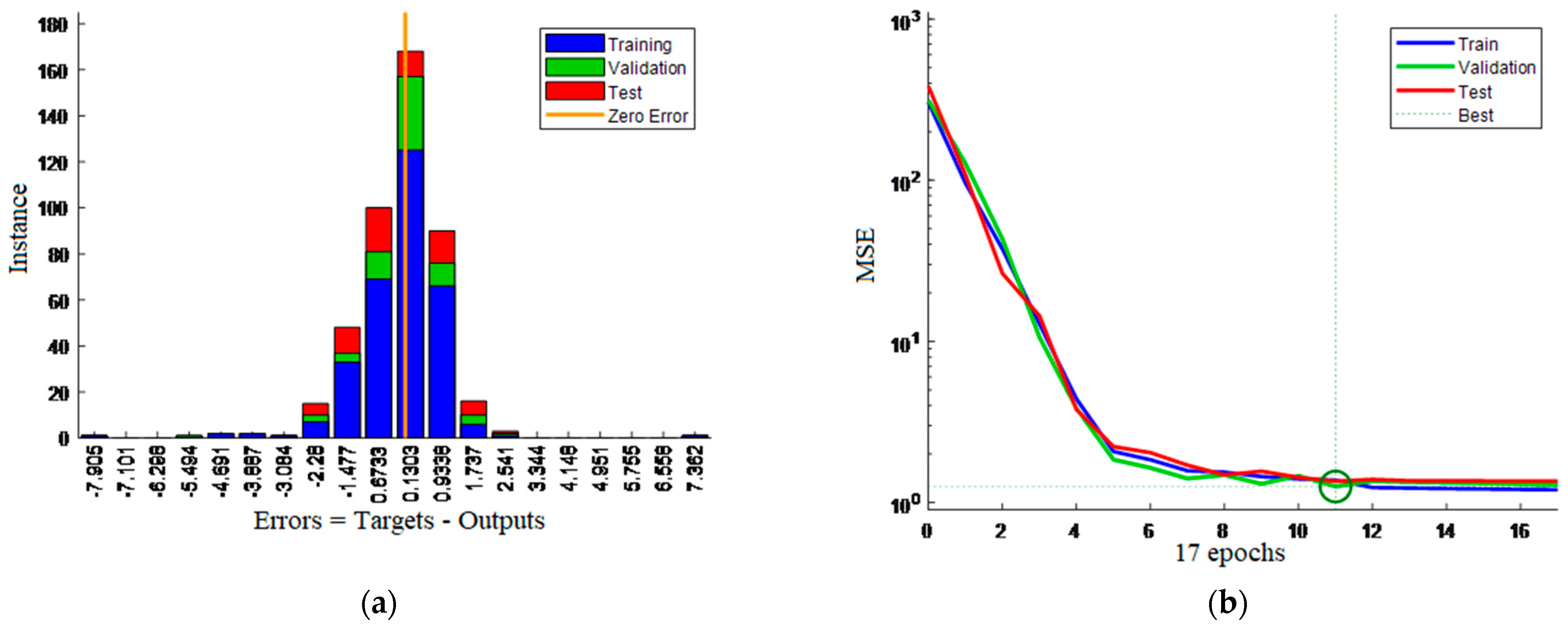
Figure 5 and Figure 6 demonstrate the effectiveness of the NN model in predicting the target values with high accuracy. Figure 5 shows the regression plots for the training, validation, and testing phases, with high correlation coefficients indicating strong predictive capability.

Figure 5. (a) Regression plot for trained NN; (b) training state plot.

Figure 6. (a) Error histogram plot for trained NN; (b) performance plot.

The proximity of the data points to the fit line reflects the model’s ability to capture underlying patterns accurately. The training state plot in the same figure illustrates the progression of key parameters like gradient, Mu, and validation checks, with the training process halting at epoch 17 due to early stopping triggered by the validation checks reaching their limit, which helped prevent overfitting.

Figure 6 complements these findings by presenting an error histogram and performance plot. The error histogram shows that the majority of prediction errors are concentrated around zero across all datasets, reinforcing the model’s accuracy. The performance plot reveals that the best validation performance, with an MSE of 1.2566, was achieved at epoch 11. The low MSE values across training, validation, and test datasets confirm that the model has a good fit. Together, these figures underscore the reliability and robustness of the model.

In the following step, the NN model obtained by the training was used for data augmentation to enhance the training dataset. The acquired model was used to estimate SSIM values for artificially generated input data. Data augmentation was performed by constructing a matrix with the following parameters as columns: TI, SI, TR, SR, and BR. The matrix was populated in such way that each row represented a unique combination of these parameters. The TI values ranged from 3 to 30 with increments of 1, while the SI values also varied from 13 to 30 in steps of 1. The TR parameter was set to one of the following values: 25, 30, 60, or 120. The SR parameter had the following values: 480, 1280, 1920, or 3840. The BR parameter’s range was determined based on the corresponding SR value: for SR = 480, BR ranged from 50 to 1000 in steps of 50; for SR = 1280, BR ranged from 50 to 3000 in steps of 50; for SR = 1920, BR ranged from 250 to 10,000 in steps of 100; and for SR = 3840, BR ranged from 700 to 10,000 in steps of 100. This method ensured that the input matrix contained a comprehensive set of unique combinations, thereby enhancing the diversity of the training data. After constructing the input matrix, the developed NN model was used to estimate output SSIM values. In total, the input matrix consisted of 548,325 × 5 values and an output array of SSIM values numbered as 548,325 values. The developed model, together with the generated input matrix and output array, is published with encoded video sequences.

4.2. Bitrate Ladder Switching Point Prediction

The augmented data provided the basis for detecting switching points to higher SR, which are essential for establishing a content-dependent bitrate ladder. The dataset that consists of switching points to a higher SR was identified through a MATLAB script that evaluated SSIM values across each SR-TR-BR combination and selected switching points for a certain SI-TI combination by identifying SR-TR-BR values at which switching to a higher SR should be carried out in order to achieve the highest possible SSIM.

Building on this, additional NNs were trained using the acquired dataset that consists of switching points to a higher SR, with one model dedicated to estimating the optimal TR (NN_TR) and another focused on optimal BR (NN_BR) estimation for a given SR switching point.

The training of NN_TR, designed to estimate optimal TR values for switching points to a higher SR, utilized SI, TI, and SR as input parameters. The idea for this NN was to estimate the optimal TR for certain SI-TI-SR combinations, i.e., the optimal value of TR for the switching point from lower SR to higher SR. From the dataset, 70% was allocated for training, 15% for validation, and 15% for testing, with the data being randomly divided. The dataset that consists of switching points to a higher SR comprised 1512 × 3 predictor variables and 1512 corresponding response variables. The Levenberg–Marquardt algorithm in MATLAB, with a network architecture consisting of ten layers, was employed for the training process for training a two-layer feedforward network with sigmoid hidden neurons and linear output neurons. The progress of the training is detailed in Table 4. The training process for the NN aimed at estimating TR demonstrated significant progress, even though it was stopped at epoch 56. The early stopping was triggered by validation checks, which is an indication that the model had reached a level of performance where further training could have led to overfitting. The reduction in performance from an initial value of 7.15 × 10³ to 133 reflects a substantial improvement, showing that the model effectively learned the underlying patterns. The gradient also decreased significantly. These results suggest that the model was well-tuned and capable of accurately predicting TR values with a high level of confidence.

Table 4. NN_TR training progress data.

Unit	Initial Value	Stop Value	Target Value
Epoch	0	56	1000
Performance (MSE)	7.15 × 103	133	0
Gradient	1.64 × 104	294	1 × 10−7
Mu	0.001	0.01	1 × 1010
Validation checks	0	6	6

The results presented in Table 5 from the NN training for TR estimation further validate the model’s robustness. The high R values across the training (0.9147), validation (0.9011), and test (0.9218) datasets indicate that the model maintains a strong predictive ability across different phases of the training process. While there was some reduction in performance during the additional tests, with R values of 0.7537 and 0.7202, these results still demonstrate that the model can be used for estimating TR based on different input data not used in the modeling process. Additional test 1 included initial data gathered during the encoding of seven video sequences used for the initial NN, and Additional test 2 incudes also data for the Lips video sequence that was not included in the training of initial NN. Overall, the NN exhibited strong performance in estimating TR, with consistent accuracy and reliability.

Table 5. Training results for NN used for estimating TR.

	Observations	R
Training	1058	0.9147
Validation	227	0.9011
Test	227	0.9218
Additional test 1	19	0.7537
Additional test 2	22	0.7202

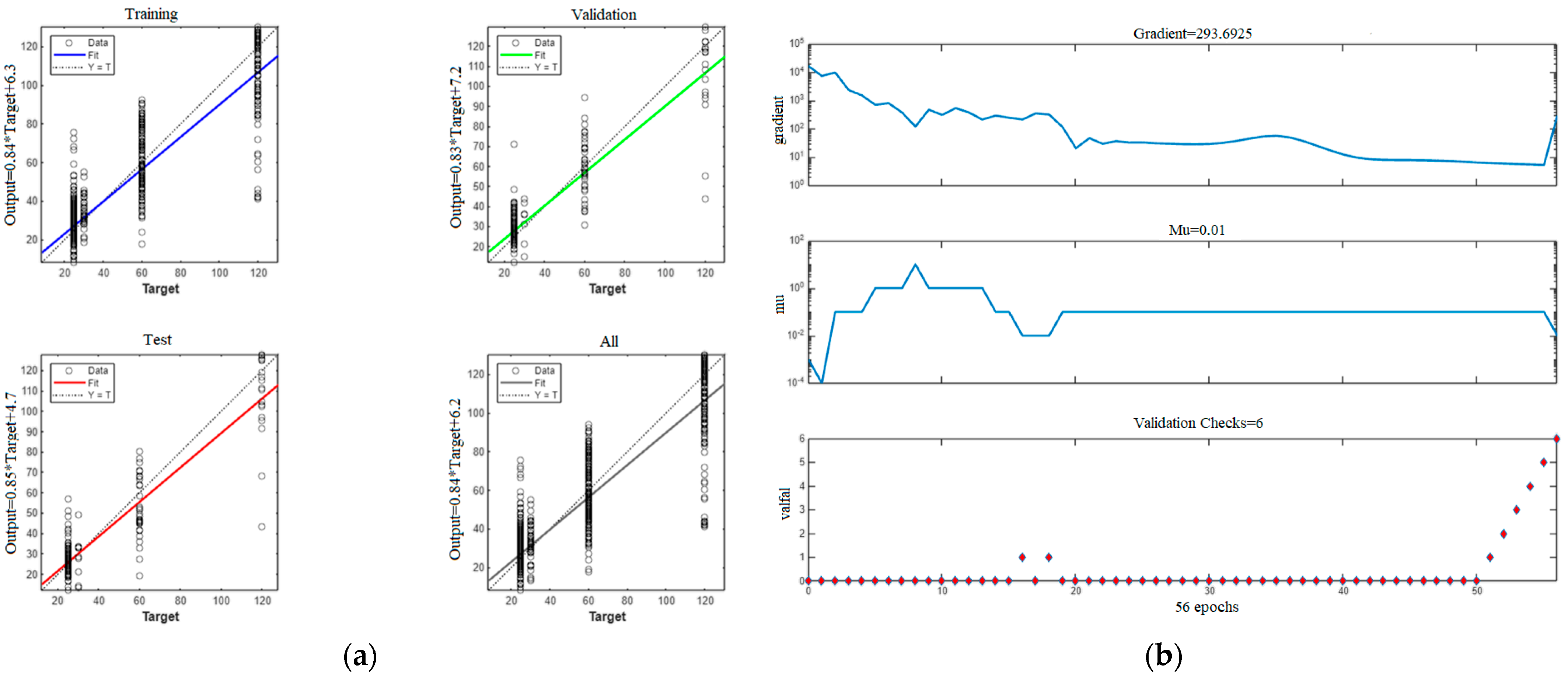
Figure 7 and Figure 8 demonstrate the strong performance of the NN in estimating bitrate TR values. Figure 7 shows the regression plot where the high correlation coefficients across the training (0.91471), validation (0.9011), and test (0.92176) datasets indicate robust predictive capability, with data points closely following the regression line.

Figure 7. (a) Regression plot for trained NN_TR; (b) training state plot.

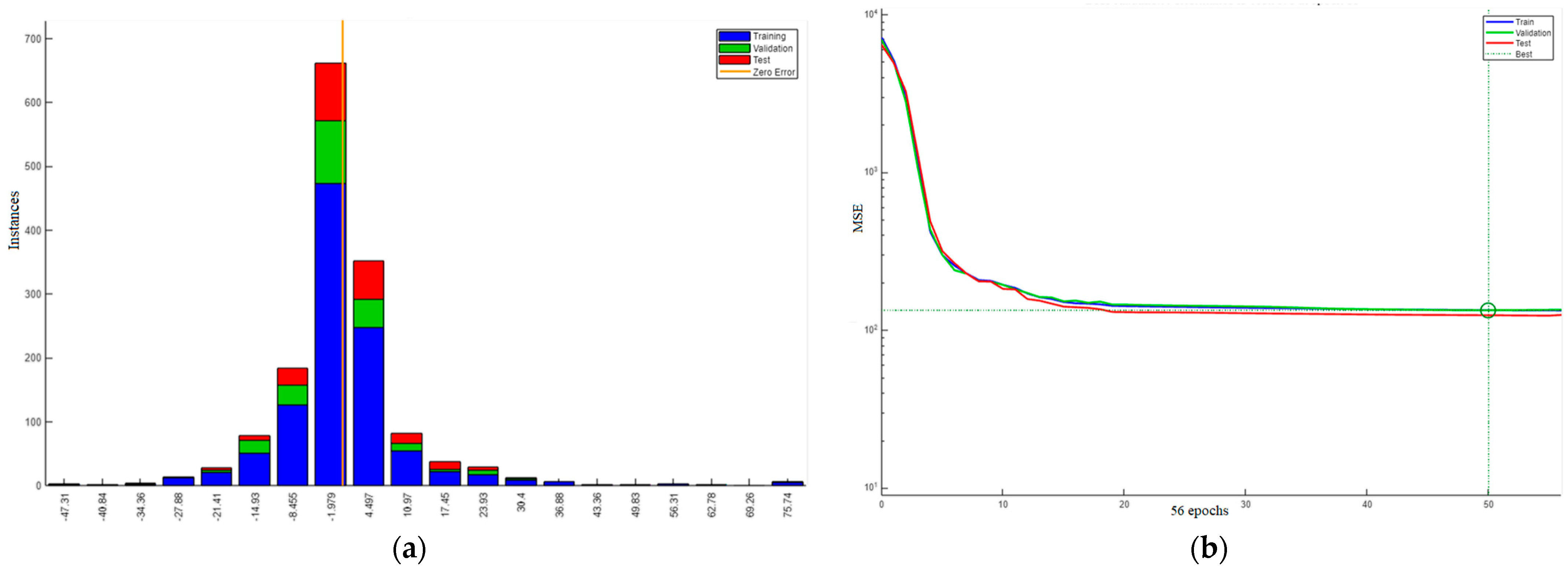
Figure 8. (a) Error histogram plot for trained NN_TR; (b) performance plot.

The training state plot reveals that the NN effectively minimized errors over time, as evidenced by the significant reduction in the performance metric and the consistent decrease in the gradient, reflecting the model’s stable convergence. Early stopping further ensured that the model did not overfit, preserving its generalizability. Figure 8 complements these findings by displaying an error histogram and performance plot. The error histogram shows that most prediction errors are centered around zero, indicating that the NN’s predictions were largely accurate. The performance plot underscores the model’s effectiveness, with low MSE values across the training, validation, and test datasets, demonstrating that the model quickly adapted to the training data and generalized well to unseen data. Overall, these figures highlight the NN’s reliability, accuracy, and strong generalization capabilities in predicting TR.

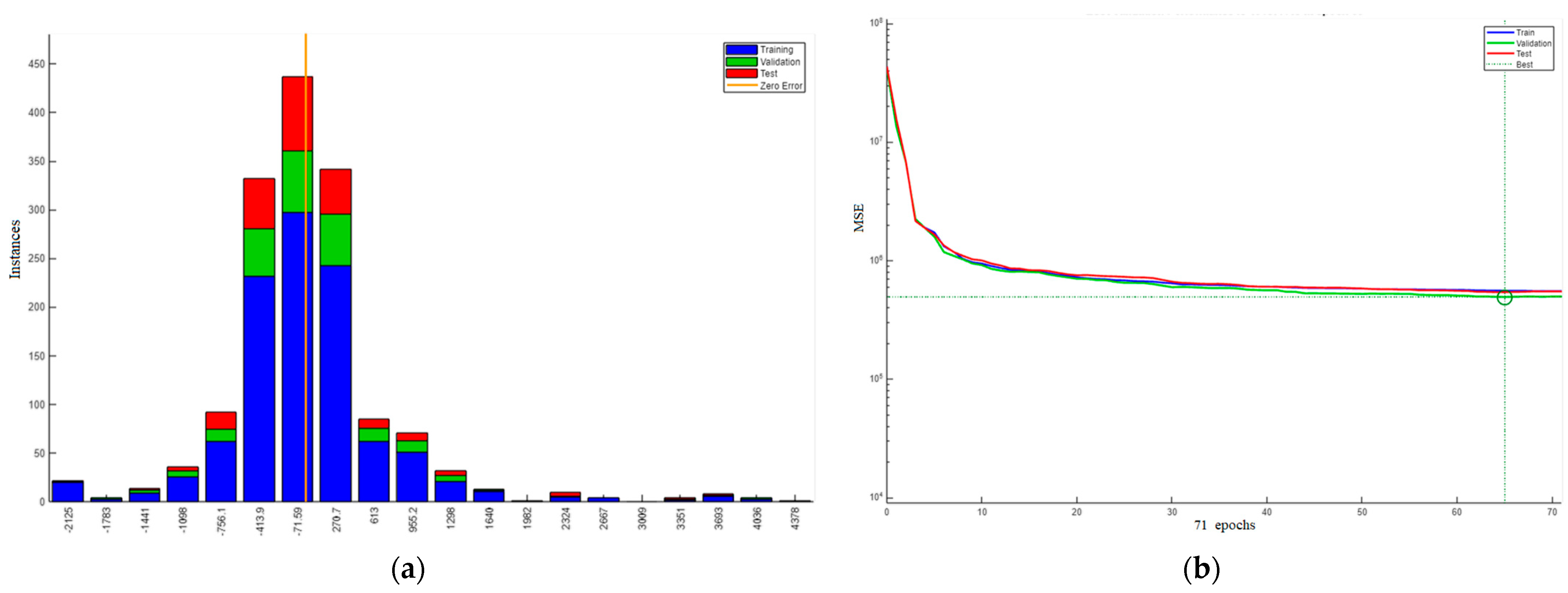
The last phase consists of training the NN_BR, aimed at estimating optimal BR values for switching points to a higher SR, using SI, TI, TR, and SR as input parameters. The idea for this NN was to estimate the optimal BR for a certain SI-TI-TR-SR combination, i.e., the optimal value of BR for the switching point from lower SR to higher SR, while taking into account the content complexity. The dataset was randomly divided, with 70% used for training, 15% for validation, and 15% for testing. This dataset that consists of switching points to a higher SR included 1512 × 4 predictor variables and 1512 response variables. The training process utilized the Scaled Conjugate Gradient algorithm in MATLAB, with a ten-layer network architecture for training a two-layer feedforward network with sigmoid hidden neurons and linear output neurons. The details of the training progress are presented in Table 6. The training process for the NN aimed at estimating BR values demonstrated a solid performance. The training was concluded at epoch 71, indicating that the model effectively learned the relationships between input parameters and target BR values within a relatively short training period. The consistent reduction in gradient values supports the model’s stable convergence towards an optimal solution. The performance results for the NN trained to estimate BR values presented in Table 7 underscore its strengths across different datasets. The model achieved moderate R values across the training (0.7482), validation (0.7827), and test (0.7703) datasets, indicating a consistent and reliable predictive performance. Notably, the model demonstrated an enhanced generalization capability in the additional tests, with R values improving to 0.8380 and 0.8404. This improvement suggests that the NN model is adept at handling new, unseen data, making it an effective tool for BR estimation in different scenarios. However, there remains potential for further enhancement, suggesting that the model’s performance could be optimized to deliver even more accurate predictions in future iterations.

Table 6. NN_BR training progress data.

Unit	Initial Value	Stop Value	Target Value
Epoch	0	71	1000
Performance	4.34 × 107	5.51 × 105	0
Gradient	6.74 × 107	8.84 × 104	1 × 10−6
Validation checks	0	6	6

Table 7. Training results for NN used for estimating BR.

	Observations	R
Training	1058	0.7482
Validation	227	0.7827
Test	227	0.7703
Additional test 1	19	0.8380
Additional test 2	22	0.8404

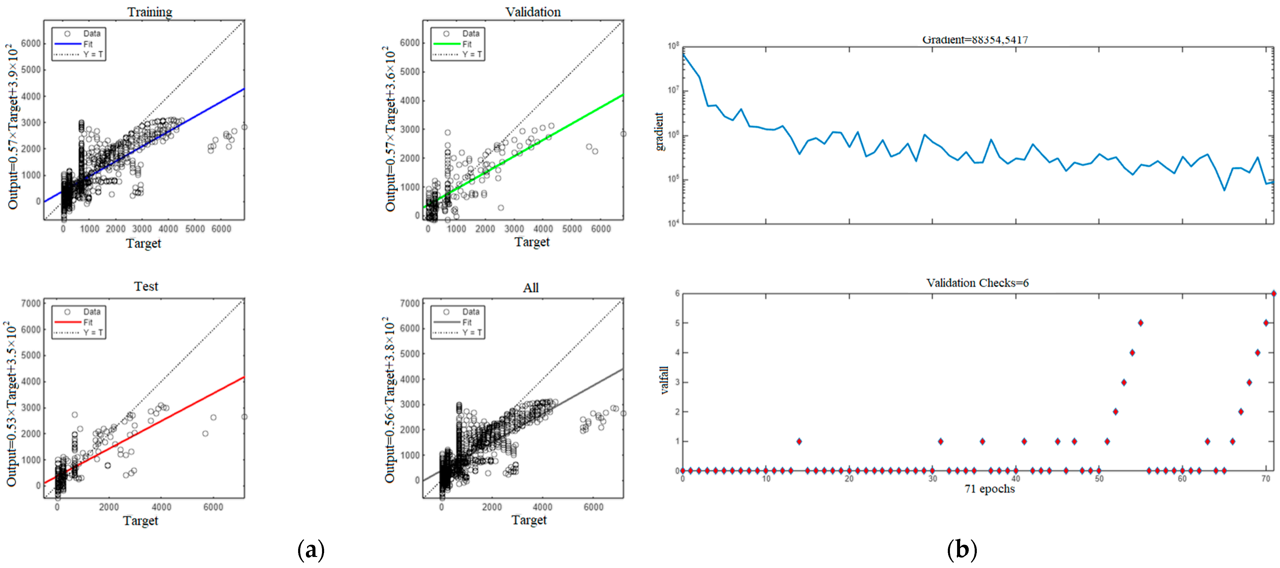
Figure 9 and Figure 10 demonstrate the performance of the NN developed for estimating BR values, revealing both strengths and areas for potential improvement. The regression plot in Figure 9a presents the model’s performance in capturing the relationship between the predicted bitrates (output) and the actual bitrates (target), with the closeness of the data points to the regression line indicating how well the model’s predictions align with the true values. The target values represent the actual bitrates that should be used for encoding, based on the optimal bitrate determined in the dataset. The output values are the bitrates predicted by the neural network. While the correlation coefficients are moderate, the model exhibits a reasonable level of accuracy across the training, validation, and test datasets, as indicated by the alignment of data points along the regression line. This suggests that the NN can capture the underlying patterns between the input features and bitrate values, albeit with some variability in predictive accuracy. Figure 9b illustrates the training state, showing a consistent decrease in performance metrics and gradient values over time, reflecting the model’s stable convergence. The early stopping mechanism was triggered after six consecutive validation steps, preventing overfitting and ensuring that the model maintained its generalization capability. This controlled convergence process highlights the effectiveness of the NN in learning from the data while preserving robustness.

Figure 9. (a) Regression plot for trained NN_BR; (b) training state plot.

Figure 10. (a) Error histogram plot for trained NN_BR; (b) performance plot.

Figure 10 further evaluates the NN_BR model’s performance, focusing on error distribution and training progress. The error histogram in Figure 10a reveals that the majority of prediction errors are concentrated around zero, demonstrating the model’s ability to generate accurate predictions. Most errors are close to zero, suggesting that the model is generally predicting bitrates accurately, although there is some variability. Figure 10b presents the performance plot, showing a progressive reduction in MSE across the training, validation, and test datasets. The low MSE values reflect the model’s efficiency in minimizing prediction errors, which further confirms the NN’s effectiveness in generalizing well to new data. Overall, while the model shows some variability in accuracy, its robustness and reliability can be seen from the correlation coefficients, low error rates, and consistent performance across different datasets.

5. Conclusions

The first key contribution of this study is the development of a new method for bitrate ladder estimation that includes the development of three neural network models. One is designed to estimate SSIM values based on SI, TI, TR, and SR, and used for data augmentation for inputs of another two NNs designed to estimate TR and BR values that represent the switching points to a higher SR. These models exhibit strong predictive performance, with correlation coefficients reaching up to 0.9452 during training and maintaining robust accuracy across validation (R = 0.9293) and testing (R = 0.9328) phases. These results suggest that the models are well trained and demonstrate effective generalization to new data.

The second contribution of this work is a novel dataset that includes encoded video sequences with temporal resolutions up to 120 fps and spatial resolutions up to 4K. This dataset fills a crucial gap in the literature, as only a limited number of such high-resolution, high-frame-rate sequences are currently available. The augmented data generated by using that dataset played a pivotal role in constructing the NN models, providing a comprehensive foundation that allowed for the accurate detection of switching points that can be used for the construction of content-dependent bitrate ladders. This approach significantly reduced the computational demands typically required for exhaustive encoding processes, making it a practical and efficient solution for real-time video streaming applications.

Looking forward, we recognize the need to expand the dataset, as the current availability of video sequences with 120 fps and 4K or higher resolution is limited to only eight sequences in the existing literature. Future work will focus on recording new video sequences that meet these high standards, further enhancing the dataset and enabling even more accurate and reliable bitrate ladder estimation. This ongoing research will continue to refine and improve adaptive video streaming technologies, offering scalable solutions for environments with varying network conditions.

References

1. Bentaleb, A.; Taani, B.; Begen, A.C.; Timmerer, C.; Zimmermann, R. A Survey on Bitrate Adaptation Schemes for Streaming Media Over HTTP. IEEE Commun. Surv. Tutor. 2019, 21, 562–585. [Google Scholar] [CrossRef]
2. Lebreton, P.; Yamagishi, K. Network and Content-Dependent Bitrate Ladder Estimation for Adaptive Bitrate Video Streaming. In Proceedings of the ICASSP 2021—2021 IEEE International Conference on Acoustics, Speech and Signal Processing (ICASSP), Toronto, ON, Canada, 6–11 June 2021; pp. 4205–4209. [Google Scholar] [CrossRef]
3. Menon, V.V.; Zhu, J.; Rajendran, P.T.; Amirpour, H.; Callet, P.L.; Timmerer, C. Just Noticeable Difference-Aware Per-Scene Bitrate-Laddering for Adaptive Video Streaming. In Proceedings of the 2023 IEEE International Conference on Multimedia and Expo (ICME), Brisbane, Australia, 10–14 July 2023; pp. 1673–1678. [Google Scholar] [CrossRef]
4. HTTP Live Streaming. Available online: https://developer.apple.com/streaming/ (accessed on 14 August 2024).
5. Sodagar, I. The MPEG-DASH Standard for Multimedia Streaming Over the Internet. IEEE MultiMedia 2011, 18, 62–67. [Google Scholar] [CrossRef]
6. Durbha, K.S.; Tmar, H.; Stejerean, C.; Katsavounidis, I.; Bovik, A.C. Bitrate Ladder Construction Using Visual Information Fidelity. In Proceedings of the 2024 Picture Coding Symposium (PCS), Taichung, Taiwan, 12–14 June 2024; pp. 1–4. [Google Scholar] [CrossRef]
7. Ge, C.; Wang, N.; Foster, G.; Wilson, M. Toward QoE-Assured 4K Video-on-Demand Delivery through Mobile Edge Virtualization with Adaptive Prefetching. IEEE Trans. Multimedia 2017, 19, 2123–2135. [Google Scholar] [CrossRef]
8. Madhusudana, P.C.; Yu, X.; Birkbeck, N.; Wang, Y.; Adsumilli, B.; Bovik, A.C. Subjective and Objective Quality Assessment of High Frame Rate Videos. IEEE Trans. Image Process. 2020, 29, 2593–2606. [Google Scholar] [CrossRef]
9. Chen, J.Y.C.; Thropp, J.E. Review of Low Frame Rate Effects on Human Performance. IEEE Trans. Syst. Man Cybern. Part A 2007, 37, 789–798. [Google Scholar] [CrossRef]
10. Huynh-Thu, Q.; Ghanbari, M. Impact of Jitter and Jerkiness on Perceived Video Quality. In Proceedings of the 2nd International Workshop on Video Processing for Consumer Electronics (VPQM 2006), Scottsdale, AZ, USA, 25–26 January 2006; pp. 1–6. [Google Scholar]
11. Zhai, G.; Cai, J.; Lin, W.; Yang, X.; Zhang, W.; Etoh, M. Cross-Dimensional Perceptual Quality Assessment for Low Bit-Rate Videos. IEEE Trans. Multimedia 2008, 10, 1316–1324. [Google Scholar] [CrossRef]
12. ITU-T, P. 910: Subjective Video Quality Assessment Methods for Multimedia Applications, Telecommunication Standardization Sector of ITU. Available online: https://www.itu.int/rec/T-REC-P.910-202310-I/en (accessed on 27 September 2024).
13. Vlaović, J.; Žagar, D.; Rimac-Drlje, S.; Vranješ, M. Evaluation of Objective Video Quality Assessment Methods on Video Sequences with Different Spatial and Temporal Activity Encoded at Different Spatial Resolutions. Int. J. Electr. Comput. Eng. Syst. 2021, 12, 1–9. [Google Scholar] [CrossRef]
14. Aaron, A.; Li, Z.; Manohara, M.; Cock, J.D.; Ronca, D. Per-Title Encode Optimization. Available online: https://medium.com/netflix-techblog/per-title-encode-optimization-7e99442b62a2 (accessed on 14 August 2024).
15. Katsavounidis, I. Dynamic Optimizer—A Perceptual Video Encoding Optimization Framework. Available online: https://netflixtechblog.com/dynamic-optimizer-a-perceptual-video-encoding-optimization-framework-e19f1e3a277f (accessed on 14 August 2024).
16. Katsenou, A.V.; Afonso, M.; Agrafiotis, D.; Bull, D.R. Predicting Video Rate-Distortion Curves Using Textural Features. In Proceedings of the 2016 Picture Coding Symposium (PCS 2016), Nuremberg, Germany, 4–7 December 2016; pp. 1–5. [Google Scholar] [CrossRef]
17. Katsenou, A.V.; Afonso, M.; Bull, D.R. Study of Compression Statistics and Prediction of Rate-Distortion Curves for Video Texture. IEEE Trans. Multimedia 2022, 101, 116551. [Google Scholar] [CrossRef]
18. Katsenou, A.V.; Sole, J.; Bull, D.R. Content-Gnostic Bitrate Ladder Prediction for Adaptive Video Streaming. In Proceedings of the 2019 Picture Coding Symposium (PCS 2019), Ningbo, China, 12–15 November 2019; pp. 1–5. [Google Scholar] [CrossRef]
19. Katsenou, A.V.; Sole, J.; Bull, D.R. Efficient Bitrate Ladder Construction for Content-Optimized Adaptive Video Streaming. IEEE Open J. Signal Process. 2021, 2, 496–511. [Google Scholar] [CrossRef]
20. Menon, V.V.; Amirpour, H.; Ghanbari, M.; Timmerer, C. Perceptually-Aware Per-Title Encoding for Adaptive Video Streaming. In Proceedings of the 2022 IEEE International Conference on Multimedia and Expo (ICME 2022), Taipei, Taiwan, 18–22 July 2022; pp. 1–6. [Google Scholar] [CrossRef]
21. Katsenou, A.V.; Zhang, F.; Swanson, K.; Afonso, M.; Sole, J.; Bull, D.R. VMAF-Based Bitrate Ladder Estimation for Adaptive Streaming. In Proceedings of the 2021 Picture Coding Symposium (PCS), Bristol, UK, 29 June–2 July 2021; pp. 1–5. [Google Scholar] [CrossRef]
22. Telili, A.; Hamidouche, W.; Fezza, S.A.; Morin, L. Benchmarking Learning-Based Bitrate Ladder Prediction Methods for Adaptive Video Streaming. In Proceedings of the 2022 Picture Coding Symposium (PCS), San Jose, CA, USA, 7–9 December 2022; pp. 325–329. [Google Scholar] [CrossRef]
23. Deng, J.; Dong, W.; Socher, R.; Li, L.J.; Li, K.; Li, F.-F. ImageNet: A Large-Scale Hierarchical Image Database. In Proceedings of the 2009 IEEE Conference on Computer Vision and Pattern Recognition, Miami, FL, USA, 20–25 June 2009; pp. 248–255. [Google Scholar] [CrossRef]
24. Bitmovin. White Paper: Per Title Encoding. Available online: https://go.bitmovin.com/en/choosing-per-title-encoding-technology (accessed on 14 August 2024).
25. Cambria. Feature: Source Adaptive Bitrate Ladder (SABL). Available online: https://www.aicox.com/wp-content/uploads/2019/07/CambriaFTC_SABL.pdf (accessed on 14 August 2024).
26. Ozer, J. A Cloud Encoding Pricing Comparison. Available online: http://docs.hybrik.com/repo/cloud_pricing_comparison.pdf (accessed on 14 August 2024).
27. Paul, S.; Norkin, A.; Bovik, A.C. Efficient Per-Shot Convex Hull Prediction by Recurrent Learning. arXiv 2022, arXiv:2206.04877. [Google Scholar]
28. MUX. Instant Per-Title Encoding. Available online: https://mux.com/blog/instant-per-title-encoding/ (accessed on 14 August 2024).
29. Kornblith, S.; Shlens, J.; Le, Q.V. Do Better ImageNet Models Transfer Better? In Proceedings of the IEEE Computer Society Conference on Computer Vision and Pattern Recognition (CVPR 2019), Long Beach, CA, USA, 16–20 June 2019; pp. 2656–2666. [Google Scholar] [CrossRef]
30. Falahati, A.; Safavi, M.K.; Elahi, A.; Pakdaman, F.; Gabbouj, M. Efficient Bitrate Ladder Construction Using Transfer Learning and Spatio-Temporal Features. In Proceedings of the 2024 13th Iranian/3rd International Machine Vision and Image Processing Conference (MVIP), Tehran, Iran, 6–7 March 2024; pp. 1–7. [Google Scholar] [CrossRef]
31. Amirpour, H.; Timmerer, C.; Ghanbari, M. PSTR: Per-Title Encoding Using Spatio-Temporal Resolutions. In Proceedings of the 2021 IEEE International Conference on Multimedia and Expo (ICME), Shenzhen, China, 5–9 July 2021; pp. 1–6. [Google Scholar] [CrossRef]
32. Song, L.; Tang, X.; Zhang, W.; Yang, X.; Xia, P. The SJTU 4K Video Sequence Dataset. In Proceedings of the 5th International Workshop on Quality of Multimedia Experience (QoMEX 2013), Klagenfurt am Wörthersee, Austria, 3–5 July 2013; pp. 34–35. [Google Scholar] [CrossRef]
33. FFmpeg. Available online: https://www.ffmpeg.org (accessed on 14 August 2024).
Disclaimer/Publisher’s Note: The statements, opinions and data contained in all publications are solely those of the individual author(s) and contributor(s) and not of MDPI and/or the editor(s). MDPI and/or the editor(s) disclaim responsibility for any injury to people or property resulting from any ideas, methods, instructions or products referred to in the content.
Article Metrics
Citations
Article Access Statistics
Multiple requests from the same IP address are counted as one view.