Semi-Supervised Learning-Enhanced Fingerprint Indoor Positioning by Exploiting an Adapted Mean Teacher Model

Abstract

Location awareness is crucial for numerous emerging wireless indoor applications. Deep learning algorithms have demonstrated the potential for achieving the required level of positioning accuracy in indoor environments. However, obtaining abundant labels for data-driven machine learning is costly in practical situations. As an effective solution to alleviating the insufficiency of labeled data for deep learning-based indoor positioning, deep semi-supervised learning (DSSL) can be employed to lessen the dependency on labeled data by exploiting potential patterns in unlabeled samples. In this paper, we propose an Adapted Mean Teacher (AMT) model within the DSSL paradigm for indoor fingerprint positioning by using a channel impulse response. To enhance the generalization of the trained model, we design an efficient implicit augmentation scheme for the training process in the AMT model. Furthermore, we develop a tailored residual network to efficiently extract location characteristics in the AMT framework. We conduct extensive simulation experiments for indoor scenarios with heavy non-line-of-sight conditions based on open datasets to demonstrate the effectiveness of our proposed AMT model. Numerical results indicate that the AMT model outperforms several consistency regularization methods and the pseudo-label method in terms of positioning accuracy and lower positioning latency, achieving a mean error of 90 cm when using a small number of labels.

1. Introduction

With the emergence of mobile device location-based services, such as the Internet of Things (IoT) and Machine Type Communication (MTC), location-based services (LBS) have been attracting intensive attention recently. As one of the most popular wireless positioning technologies, the Global Navigation Satellite System (GNSS) has achieved great success in outdoor open-scene positioning. However, GNSS becomes infeasible for indoor scenarios due to the signal strength attenuation and multi-path effects [1]. Thus, it is imperative to develop efficient indoor positioning schemes to meet the requirements of numerous and booming indoor location-aware applications, such as indoor emergency rescue, smart factory asset management and tracking, mobile medical services, virtual reality games, etc.

Traditional positioning methods can be roughly categorized as geometry-based and feature-matching-based methods [2]. The geometry-based methods, such as Angle of Arrival (AOA), Angle of Departure (AOD), Time Difference of Arrival (TDOA), and Multi-Round Trip Time (Multi-RTT), rely on the measurement of positioning information and estimation of the target location. Feature matching-based methods are mainly regarded as fingerprint recognition methods, which have also received widespread attention in positioning technology in the era of 5G and beyond [3]. Specifically, the primary approach of fingerprint recognition is based on the Received Signal Strength (RSS) or Channel State Information (CSI) [4].

Recently, the 3rd Generation Partnership Project (3GPP) emphasized the importance of the LBS in 5G networks, and in 3GPP Rel-16, it ultimately established the direction of 5G positioning enhancement [5]. Specifically, the New Radio (NR) specification includes reference signals introduced for positioning. These signals include the Positioning Reference Signal (PRS) for the downlink and the Sounding Reference Signal (SRS) for the uplink. Based on these signals, 3GPP Rel-16 has introduced a number of advanced positioning schemes suitable for 5G NR, including angle-based positioning schemes based on downlink AOD or uplink AOA, downlink TDOA, uplink TDOA, and Multi-RTT.

Although these methods can provide high positioning accuracy, they heavily depend on the availability of line-of-sight (LOS) components [6]. Unfortunately, in many indoor scenarios, such as the industrial environment, there could be many obstacles that can cause signal refraction, reflection, and diffraction, which leads to poor performance under some specific scenarios [7]. Hence, it is imperative to explore efficient techniques to improve the positioning performance in heavy non-line-of-sight (NLOS) scenarios for the 5G system and beyond.

In order to achieve higher positioning accuracy, the standardization work of 3GPP Rel-18 is introducing Carrier Phase Positioning (CPP) technology. The carrier phase information of a signal contains distance information between the signal receiver and transmitter, which can be used to accurately calculate the user’s position. CPP technology has been widely applied in GNSS, enabling centimeter or even millimeter-level positioning accuracy [8]. However, the low power of the GNSS signals can be blocked and discontinuous in indoor scenarios. Due to the high power of cellular network signals and their resistance to environmental interference, carrier phase positioning based on cellular signals is not limited to outdoor environments, and because the carrier phase contains the distance between the signal receiver and transmitter, it can be used to precisely calculate targets’ position [1]. Compared to satellite-based CPP, using CPP in indoor scenarios can achieve similar positioning accuracy and lower positioning latency. In the measurement of the carrier phase from the Positioning Reference Signal (PRS), the estimated value of the Channel Frequency Response (CFR) is first used to obtain the Channel Impulse Response (CIR) by an Inverse Discrete Fourier Transform (IDFT). Then, based on certain criteria, the first path of arrival is determined from the CIR, and the phase is calculated to obtain the carrier phase measurement value. Therefore, the CIR signal can be considered as the original information of the carrier phase to distinguish multipath characteristics and can potentially be used for accurate and pervasive indoor positioning [9]. In addition, CSI can be also obtained from CFR, which is the sampled version of CFR at the granularity of the subcarrier level [9].

Meanwhile, in recent years, Artificial Intelligence (AI) has experienced rapid development and widespread applications in positioning fields due to their outstanding performance [10]. 3GPP also studied AI-based positioning enhancement for indoor scenarios [11]. The AI-based solutions can potentially overcome the limitations and difficulties of traditional positioning methods, and numerical results show that deep supervised learning with CIR information can greatly improve positioning accuracy compared with traditional methods [12].

Motivated by the high performance of AI and its wide application, some research has regarded CSI as image information and finds a mapping from CSI measurements to the coordinates of the target terminals by using deep learning; these learning-based methods achieved higher positioning accuracy than traditional positioning methods [13,14]. Meanwhile, In CSI-based or CIR-based fingerprinting approaches, AI models are able to learn the knowledge of fingerprint features offline based on the dataset of labeled fingerprints [4]. However, obtaining a large amount of labeled data is difficult and rather costly due to the need for experts’ time and experience. Moreover, low-quality labeled data can adversely affect the performance of deep models. To address these issues, Deep Semi-Supervised Learning (DSSL) has been recently considered to improve learning performance by exploring potential patterns from unlabeled samples.

When carefully examining the similarity of image processing and the underlying indoor location, we can find that both image processing and CIR positioning are based on feature recognition, thereby realizing the perception and understanding of user location, and obtaining position features of User Equipments (UEs) in a specific area. They also have similar feedback mechanisms in the process of model training through generating loss values when using a neural network. These observations inspire us to exploit an adapted DSSL method to handle indoor positioning tasks. Although various methods, such as the $\mathrm{\Pi }$ Model, Temporal Ensembling [15], and Mean Teacher [16], have shown advantages for image classification, some modifications have to be made based on the data type and target format for positioning tasks. In this paper, we develop an Adapted Mean Teacher (AMT) model under the DSSL paradigm for indoor positioning using CIR fingerprints, which is inspired by the inherent similarity between image processing and indoor positioning, and the efficiency of the consistency regularization method. Additionally, the 5G Advanced has set high requirements for future positioning accuracy, aiming to achieve centimeter-level precision. Based on the scenario of a 5G new radio, we aim to apply the machine learning method to indoor positioning to meet the development needs of 5G Advanced. The main contributions of this paper can be summarized as follows:

• We mathematically present the CIR estimation for building a CIR-based fingerprint dataset according to the 5G NR standard.
• A tailored neural network based on Residual Network (ResNet) is designed to extract position features of CIR fingerprints to predict the position of users. In a supervised learning manner with abundant label data, it achieves sub-meter level accuracy with a mean error of 31 cm.
• We propose efficient implicit random augmentation methods for CIR data by borrowing the idea of data augmentation in image processing tasks. Experiments on adding augmentation methods in the training process show that our proposed method can achieve higher accuracy in both supervised and semi-supervised learning methods.
• We propose an AMT model to handle fingerprint indoor positioning tasks and possess a superior positioning performance than reference algorithms, achieving a sub-meter level accuracy.

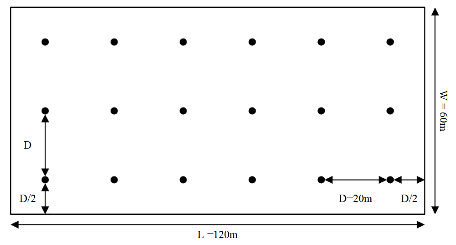
The rest of this paper is organized as follows. Section 2 presents the related works for positioning methods and existing DSSL methods. Section 3 presents the scenario and system model. Section 4 elaborates the proposed AMT model, and in Section 5, we provide a detailed description of the CNN structure. We present simulation results as well as discussions in Section 6 and finally conclude the paper in Section 7.

2. Related Works

Positioning technology has been developing for decades. During this time, various location technologies have emerged. To summarize the previous technical work, in this section, we start by summarizing positioning techniques based on the common metrics of positioning. We then review recent research advancements in wireless positioning systems, which contain a detailed explanation of positioning technology for 5G cellular networks related to the paper’s topic. Additionally, we provide an overview of AI-based indoor positioning methods and DSSL-based indoor positioning schemes.

2.1. Positioning Techniques Based on Common Measurements

Indoor positioning is a challenging problem that has been extensively investigated, resulting in the development of various technologies such as WiFi, Bluetooth, Ultra-Wideband (UWB), geomagnetism, sound/ultrasound, or Pedestrian Dead Reckoning (PDR) [8,17]. Though a number of facilities can be used for positioning, in traditional positioning schemes for both cellular and non-cellular positioning systems, some universal signal measurements are used. In this section, we introduce positioning methods based on common measurements such as RSS, AOA, and TDOA.

The RSS-based approach [18] is a simple and commonly used method for indoor positioning, which involves measuring the strength of the received signal. By using signal propagation models with the knowledge of the transmission power or power at a reference point, it is possible to estimate the absolute distance between the two devices based on the RSS value. In the device-based positioning, RSS positioning requires the use of trilateration or N-point lateration [19]. This involves using the RSS at the UE to estimate the precise distance between a UE and three or more signal sources. Subsequently, basic geometry and trigonometry are applied to determine the location of the device relative to the reference points.

The AOA-based methods [20] make use of antenna arrays on the receiver side to determine the angle that the transmitted signal arrives at the receiver. This is achieved by calculating the TDOA at each element of the antenna array. While AOA can provide an accurate estimation for short distances between the transmitter and receiver, it requires more complex hardware and precise calibration compared with RSS techniques. Additionally, the accuracy of the AOA-based positioning decreases as the distance between the transmitter and receiver increases, as even a small error in the angle calculation can result in a significant error in the actual location estimation. Furthermore, in an indoor environment with multipath effects, obtaining the LOS condition for AOA-based positioning can be challenging.

The TDOA-based methods [21] use the differences in signal propagation time measured at the receivers from different transmitters. To accurately determine the location of the receiver, the TDOAs from at least three transmitters are required. This allows for the calculation of the receiver’s position as the intersection of three or more hyperboloids [21]. Solving the system of hyperbola equations can be achieved through methods such as linear regression or by linearizing the equation using Taylor-series expansion.

However, all of the aforementioned existing methods heavily depend on LOS scenarios, and in other scenarios, such as urban streets and indoor scenarios, the complex signal propagation paths will lead to unreliable positioning results.

2.2. Wireless Positioning Systems

Wireless positioning technology can be categorized based on the scope of service, including positioning systems for Wireless Wide Area Network (WWAN) and Wireless Local Area Network (WLAN)/Personal Area Network (PAN). The WLAN/PAN includes WiFi positioning systems, Bluetooth positioning systems, and UWB positioning systems, while the WWAN includes GNSS and cellular network positioning systems.

WiFi-based positioning technologies mainly consist of four types, including positioning methods based on RSS, fingerprinting, AOA, and TOA. Different from traditional RSS-based WiFi positioning systems, the use of deep learning methods has been widely applied to explore the numerical features of signals in RSSI positioning. Dai et al. [22] used a multi-layer neural network (MLNN) to provide localization services in RSS-based indoor localization, which combined the RSS signal-transforming section, raw data-denoising section, and node-locating section to form a deep architecture. By using the deep architecture, the predicted locations of UE can be attained without using a radio pathloss model or comparing with a radio map. Hoang et al. [23] emphasized the superiority of RNN in dealing with location nonlinearly because the mapping from RSS to UE’s location is nonlinear. In this work, the authors provided a complete study of several RNN architectures for WiFi RSS fingerprint positioning. Research on WiFi fingerprint positioning typically utilizes the CSI or RSS signals obtained from WiFi signals [24]. The CSI-based method provides more detailed signal propagation characteristics, resulting in better positioning accuracy compared to RSS [25]. However, the acquisition of CSI requires the cooperation of WiFi access points (APs), which is limited by the practical deployment of devices. To overcome this obstacle, Gao et al. [26] proposed a CSI fingerprinting-based positioning approach named CRISLoc, which obtains the packets in the air passively, while a joint clustering and outlier detection method is used to find altered APs. By applying CRISLoc, the accuracy of CSI fingerprinting-based localization can reach a sub-meter level. The RSS-based WiFi fingerprint positioning technology is often heavily influenced by noisy environments; recent studies have begun to utilize advanced deep-learning models to address these issues. Chen et al. [27] proposed an LF-DLSTM framework to alleviate the noise effect and attain stable features from the raw noisy RSS data. Additionally, in traditional AOA WiFi positioning systems, a limited number of antennas in WiFi devices can result in limited AOA resolution. In order to achieve more accurate and robust positioning, recent research has focused on developing new methods. Yang et al. [28] worked out the relationships among different AoAs of different APs, and proposed a novel co-localization method between multiple APs to achieve a real-time and accurate localization system. For TOF-based WiFi positioning, the positioning performance of the TOF-based WiFi system is largely limited by the WiFi channel bandwidth because of the low resolution of TOF, and recent research has utilized multipath to increase time resolution [29]. While the use of WIFI technology for positioning facilities can achieve centimeter-level accuracy in many studies, the coverage range is limited to a 10 m level, which results in extremely high deployment costs when attempting to cover large areas.

The Bluetooth positioning system is a common short-distance wireless communication technology primarily used for PAN. In the latest release of Bluetooth 5.1, the version has added measurements of AOA and AOD, integrating the results with RSS to provide sub-meter positioning accuracy [30]. However, Bluetooth positioning faces serious multipath interference issues. The accuracy of positioning is difficult to further improve, and there are limitations on coverage range, making it challenging to deploy over large areas [31].

UWB positioning technology is characterized by high positioning accuracy, high rating, and strong resistance to multipath interference [32]. Current recent research has mainly focused on how to reduce the impact of non-line-of-sight (NLOS) paths in high NLOS scenarios when applying UWB positioning to decrease positioning errors. Poulose et al. [33] applied LSTM networks in UWB localization in indoor scenarios to migrate the negative effects from both NLOS conditions and TOA errors. Compared to the conventional method, it can reduce the mean position error to 7 cm. Although UWB has a high positioning accuracy, the high cost of base stations and tags for UWB positioning makes it not a universally applicable positioning solution.

For positioning systems in WWAN, Assist-Global Positioning System (A-GPS) technology is widely used in the location services of smartphones. It leverages cellular mobile communication networks to broadcast GNSS information and its auxiliary data, thereby assisting UEs in shortening the satellite’s initial search time and improving location accuracy during satellite navigation [34]. The GNSS signal can be easily blocked, and recent research has attempted to enhance GPS using the UWB systems. Gao et al. [35] proposed an RCP scheme that evaluates the positioning performance by generating a dataset in real urban scenarios. Experimental results show that this scheme can robustly resist adverse effects on positioning performance.

Positioning technologies in cellular networks have evolved from 2G to 5G, and now to 5G NR and 5G-Advanced. In 5G NR and 5G-Advanced, the requirement for positioning accuracy has reached to centimeter level, leading to a significant focus on research based on CSI and CPP. Meanwhile, some studies have emphasized machine learning and fingerprint recognition. Zhang et al. [36] developed a novel Attention-Aided Residual Convolutional Neural Network (AAresCNN) for CSI-based indoor positioning, achieving a state-of-the-art performance on public datasets. Ruan et al. [37] proposed a novel positioning system, iPOS, using commercial 5G-NR CSI fingerprints for indoor positioning, incorporating CSI pre-processing and feature reconstruction modules. In the current development of 5G-Advanced, Tedeschini et al. [38] utilized CIR to extract position-related features and enhance positioning accuracy through cooperative deep learning, combined with NLOS recognition. Unlike other positioning systems, cellular network positioning does not require additional infrastructures and can achieve centimeter-level accuracy, which significantly reduces positioning costs. The use of CSI and CPP as measurement values, along with machine learning positioning strategies, demonstrates advancements in both 3GPP standards and recent research.

2.3. DSSL Methods for Indoor Positioning

In recent years, deep learning algorithms have shown great potential in solving complex positioning problems, and DSSL methods have been emerging as a promising approach to deal with the challenges of limited labeled data in positioning problems by leveraging both labeled and unlabeled data to train deep learning models.

The branches of DSSL mainly include pseudo-label methods [39], deep generative methods [40], graph-based methods [41], consistency regularize methods [15,16] and hybrid methods [42]. Currently, research on DSSL mainly focuses on the image classification task.

For DSSL methods applied in image classification tasks, each branch has advanced algorithms capable of achieving high accuracy. Regarding the pseudo-labeling method, using the high-confidence model’s predictions as pseudo labels for unlabeled samples is a common approach known as self-training. Ref. [39] proposed a simple and efficient training framework for neural networks. The model is first trained in a usual supervised manner; this trained model is used to attain predictions from unlabeled data. The crossentropy loss is used in the process of obtaining predictions from unlabeled samples, and when we obtain soft labels, the model’s highest confidence predictions are viewed as pseudo labels.

Consistency regularization is a technique that typically involves using a single model to make multiple predictions with different input noise or model parameters each time. It aims to obtain a similar prediction result under different noisy inputs and parameters, thereby improving the generalization of the model. From certain perspectives, using consistency regularization can also be observed as generating pseudo-labels. However, it focuses on obtaining accurate labels by regularizing the distance between outputs and supervised training, which is fundamentally different from the pseudo-labeling method. Ref. [15] proposed two training frameworks, named $\mathrm{\Pi }$ Model and Temporal Ensembling, respectively. During each epoch of training with the $\mathrm{\Pi }$ Model, the same batch of unlabeled samples is processed by the same model twice after adding random perturbations. Some inconsistencies in the two predictions will exist because of the different perturbations, so the $\mathrm{\Pi }$ Model uses a consistency loss function to minimize the disparity between the two predicted outputs. Temporal Ensembling makes some improvements to the $\mathrm{\Pi }$ Model. Due to the fact that the $\mathrm{\Pi }$ Model requires two rounds of inference at each step, it slows down the inference speed. To overcome this defect, the Temporal Ensembling model only needs one round of inference, while one prediction is obtained by calculating the moving average of a historical output over a certain period of time. Another prediction is generated by the current output. By combining the loss items of two predictions as a loss function, the inconsistency in the two predictions decreases.

Mean Teacher [16] is an improved method for Temporal Ensembling, and it consists of a teacher model and a student model. The student model resembles the $\mathrm{\Pi }$ Model, while the teacher model shares the same structure as the student model but incorporates Exponential Moving Average (EMA) of the student weights. This allows Mean Teacher to enforce a consistency constraint between the predictions of the student and teacher models. Results from [16] indicate that Mean Teacher performs superiorly in test accuracy compared to Temporal Ensembling, while it also allows for training with fewer labels.

DSSL-based indoor positioning is often considered as a regression problem rather than a classification problem, and previous research on DSSL for indoor positioning mainly focuses on pseudo-label methods [43], deep generative methods [44], and graph-based methods [45]. The idea of the pseudo-label method in [43] is to pretrain the initial model with labeled data and use the trained model to predict unlabeled data, treating the predictions as pseudo-labels. The advantage of this method is its simplicity and strong operability, which is needless to deploy additional models. Whereas in actual positioning scenarios, the target distributions of labeled data and unlabeled data are often inconsistent, and using the same model parameters directly on different distributed data will reduce the positioning accuracy. In [44], the author discussed a semi-supervised indoor positioning scenario based on the Generative Adversarial Network (GAN) by using CSI data, which consists of a generator and a discriminator and aims to generate new CSI that similar to labeled data. Results of using GAN for semi-supervised positioning have confirmed its effectiveness under a few labeled input. However, using explicit data augmentation methods to improve the performance of positioning may increase the computing power burden of the device and consume a large amount of memory when facing the massive data demand. Moreover, when the labeled data are highly resembled, overfitting can be caused by a deep generative method. Moreover, the consistency regularization method as an effective DSSL method achieves a good balance between accuracy and memory occupation. In [46], the ladder network, the first attempt at consistency regularization, was used for indoor positioning using CSI, which is inspired by a deep denoising AutoEncoder. It predicts whether each input has noise, using denoising functions and the unsupervised denoising square to generate consistency loss, and aligns with the supervised learning loss to obtain more accurate user coordinates.

The advanced consistency regularization methods after the Ladder Network, such as the $\mathrm{\Pi }$ Model, Temporal Ensembling, and Mean Teacher, have been proposed to improve accuracy without requiring additional data by regulating the consistency loss between noisy inputs to reduce overfitting and enhance the generalization of neural networks. However, these methods have not been really well used yet, and how to efficiently apply them to the positioning field still remains outstanding.

3. Scenario and System Model

3.1. Scenario Description

We consider the positioning in a general indoor scenario, such as a factory, as shown in Figure 1. A number of Base Stations (BSs) are deployed on the ceiling of the factory with a certain area, and each BS consists of one microcell with an omni-directional antenna towards the ground. The dense clutters are randomly distributed, and heavy NLOS propagations exist in such complex scenarios. The clutter in the scenario can be considered as machinery, assembly lines, and storage shelves. UEs are randomly distributed in the factory while receiving the reference signal, e.g., PRS sent by BSs and process channel estimation for deriving CIR.

Figure 1. Schematic diagram of indoor positioning scenario.

3.2. Channel Model

We assume a massive multiple-input multiple-output (MIMO) system for presenting CIR, where each BS is equipped with $N_t$ transmission antennas (Tx), and each UE has $N_r$ receiving antennas (Rx). In a different environment, the mobile radio propagation link between BS and UE could be LOS or NLOS. To establish CIR, we use 3D channel models to express the channel coefficients between each Tx and Rx according to 3GPP TR 38.901 [47]. For each link, let there be Z clusters, each with M rays. We use $m\in \{1,2,\dots ,M\}$ to denote the index of a specific ray. For the NLOS case, when cluster $\zeta$ belongs to the $Z-2$ weakest clusters represented as $\zeta \in \{3,4,\dots ,Z\}$, the power of different rays in each cluster is equal. The channel coefficient of ray m in cluster $\zeta$ for the receiver and transmitter antenna element pair u, s can be expressed as

$$\begin{array}{c}{H}_{u,s,\zeta ,m}^{NLOS}\left(t\right)=\sqrt{{\displaystyle \frac{P_{\zeta }}{M}}}{\left[\begin{array}{c}{F}_{rx,u,\theta }\\ F_{rx,u,\varphi }\end{array}\right]}^T\left[\begin{array}{cc}{e}^{j{\mathrm{\Phi }}_{\zeta ,m}^{\theta \theta }}& \sqrt{{\kappa }_{\zeta ,m}^{-1}}{e}^{j{\mathrm{\Phi }}_{\zeta ,m}^{\theta \varphi }}\\ \sqrt{{\kappa }_{\zeta ,m}^{-1}}{e}^{j{\mathrm{\Phi }}_{\zeta ,m}^{\varphi \theta }}& e^{j{\mathrm{\Phi }}_{\zeta ,m}^{\varphi \varphi }}\end{array}\right]\\ \left[\begin{array}{c}{F}_{tx,s,\theta }\\ F_{tx,s,\varphi }\end{array}\right]\mathtt{exp}({\displaystyle \frac{j2\pi ({\widehat{r}}_{rx,\zeta ,m}^T{\overline{d}}_{rx,u}+{\widehat{r}}_{tx,\zeta ,m}^T{\overline{d}}_{tx,s}+{\widehat{r}}_{rx,\zeta ,m}^T\overline{v}t)}{{\lambda }_0}}),\end{array}$$

(1)

where $P_{\zeta }$ stands for the power of the cluster, $F_{rx,u,\theta }$, and $F_{rx,u,\varphi }$ is the field pattern of u in the direction of the spherical basis vectors, $\theta$ and $\varphi$, respectively. $F_{tx,s,\theta }$ and $F_{tx,s,\varphi }$ are the field patterns of s in the direction of $\theta$ and $\varphi$, respectively. ${\widehat{r}}_{tx,\zeta ,m}^T$ is the spherical unit vector with an azimuth arrival angle and elevation arrival angle, and ${\widehat{r}}_{rx,\zeta ,m}^T$ is the spherical unit vector with an azimuth departure angle and elevation departure angle. (${\overline{d}}_{rx,u}$, ${\overline{d}}_{tx,s}$) is the location vector of u and s, ${\kappa }_{\zeta ,m}$ is the cross-polarization power ratio in a linear scale, and ${\lambda }_0$ is the wavelength of the carrier frequency. $\mathrm{\Phi }$ represents the random initial phase for different polarization combinations, and $\overline{v}$ is the velocity vector of the UE.

For the LOS case, the channel coefficient is given by:

$$\begin{array}{c}{H}_{u,s,1}^{LoS}\left(t\right)={\left[\begin{array}{c}{F}_{rx,u,\theta }\\ F_{rx,u,\varphi }\end{array}\right]}^T\left[\begin{array}{cc}1& 0\\ 0& -1\end{array}\right]\left[\begin{array}{c}{F}_{tx,s,\theta }\\ F_{tx,s,\varphi }\end{array}\right]\mathtt{exp}(-j2\pi {\displaystyle \frac{d_{3D}}{{\lambda }_0}})\\ \mathtt{exp}({\displaystyle \frac{-j2\pi ({\widehat{r}}_{rx,LoS}^T{\overline{d}}_{rx,u}+{\widehat{r}}_{tx,LoS}^T{\overline{d}}_{tx,s}+{\widehat{r}}_{rx,LoS}^T\overline{v}t}{{\lambda }_0}}),\end{array}$$

(2)

where $d_{3D}$ represents the 3D distance between Tx and Rx.

3.3. Estimation of Channel Impulse Response

In order to better capture the characteristics of the natural channel environment, the two strongest clusters $\zeta \in \{1,2\}$ are spread to three different sub-clusters with fixed delay offsets. The M rays within a cluster are mapped to sub-clusters $\xi \in \{1,2,3\}$, and are divided into three groups $R_{\xi }$, each with a power $R_{\xi }/M$ and delay offset ${\tau }_{\zeta ,\xi }-{\tau }_{\zeta }$ for a NLOS channel. Then, the CIR from s to u in the NLOS case can be expressed as

$$\begin{array}{c}\hfill H_{u,s}^{NLoS}(\tau ,t)={\displaystyle \sum _{\zeta =1}^2}{\displaystyle \sum _{\xi =1}^3}{\displaystyle \sum _{m\in R_{\xi }}}{H}_{u,s,\zeta ,m}^{NLoS}\left(t\right)\delta (\tau -{\tau }_{\zeta ,\xi })+{\displaystyle \sum _{\zeta =3}^Z}{H}_{u,s,\zeta }^{NLoS}\left(t\right)\delta (\tau -{\tau }_{\zeta }),\end{array}$$

(3)

where $H_{u,s,\zeta }^{NLoS}\left(t\right)$ represents the channel coefficient of cluster $\zeta$ for the antenna pair $u,s$, which is formulated as $H_{u,s,\zeta }^{NLoS}\left(t\right)={\sum }_{m=1}^M{H}_{u,s,\zeta ,m}^{NLoS}\left(t\right)$. In the LOS case, by adding the LOS channel coefficient to the CIR in the NLOS case and adjusting the scaling factor $\gamma$, we obtain the CIR, as follows:

$$H_{u,s}^{LoS}(\tau ,t)=\sqrt{\frac{1}{\gamma +1}}{H}_{u,s}^{NLoS}(\tau ,t)+\sqrt{\frac{\gamma }{\gamma +1}}{H}_{u,s,1}^{LoS}\left(t\right)\delta (\tau -{\tau }_1),$$

(4)

where $H_{u,s,1}^{LoS}\left(t\right)$ represents the LOS channel coefficient with the strongest power transmission when cluster $\zeta =1$, and ${\tau }_1$ symbolizes the minimum delay of arrival. Note that positioning mainly depends on the CIR in the NLOS case because a heavy NLOS environment exists in the scenario.

3.4. Problem Formulation

In the indoor positioning scenario, we represent the UE set as $X={\left\{x_n\right\}}_{n=1,\dots ,N}$. The real global coordinate of UE n in the indoor area is denoted as $P_{true}^i=[P_h^n,P_v^n]$, where $P_h^n$, $P_v^n$ represent the horizontal coordinate and vertical coordinate respectively. Assuming that the coordinate of each UE predicted by the neural network $f(·)$ is valid, the problem can be restated as finding a way to utilize CIR information, the neural network $f(·)$, and the true position $P_{true}$ of each UE to approximate the global coordinate.

Let the predicted coordinate for UE n with the position error be denoted as $f(\theta ,x_n)$, where $\theta$ represents the weights of the neural network. The position error is defined as $|f(\theta ,x_n)-P_{true}^n|$. Our optimization objective for a set of N training samples is to minimize the Mean Squared Error (MSE) value between the predictions and true labels, which can be expressed as:

$$min{\displaystyle \frac{1}{N}}\sum _{n=1}^N{(f(\theta ,x_n)-P_{true}^n)}^2.$$

(5)

4. Semi-Supervised Learning Based on Mean Teacher Model

The concept of consistency regularization is that even if the input is perturbed, the network can still generate an output consistent with the output before perturbating and punishing inconsistent items. Specifically, consistency is based on the comparison of output space distributions, which is referred to as an approximate result or an output vector with a small distance from distribution. Consistency regularization is mainly applied to the teacher–student structure, with a consistency constraint defined as:

$${\mathbb{E}}_{x\in X}\mathcal{D}(f_s({\theta }_s,{\eta }_s,x_s),f_t({\theta }_t,{\eta }_t,x_t)),$$

(6)

where $f_s({\theta }_s,{\eta }_s,x_s)$ is the student’s prediction of input $x_s$, $f_t({\theta }_t,{\eta }_t,x_t)$ is the teacher’s prediction of input $x_t$. $\mathcal{D}(·)$ is the distance function between two vectors. Different consistency regularization methods differ in the way they generate consistency constraints. For example, the $\mathrm{\Pi }$ Model [15] generates consistency a constraintbetween two predictions of the same model by adding different noises to inputs, and the Temporal Ensembling [15] generates constraint between the training prediction of the current epoch and EMA prediction from the last epoch. As for the Mean Teacher, it averages model weights instead of predictions. Specifically, the teacher model uses the EMA weights of the student model and then generates a constraint between the teacher model’s prediction and the student model’s prediction. The consistency constraint of the Mean Teacher can be defined as

$${\mathbb{E}}_{x,{\eta }_s,{\eta }_t}\mathcal{D}(f_s(\theta ,{\eta }_s,x),f_t(\mathit{EMA}\left(\theta \right),{\eta }_t,x)),$$

(7)

where ${\eta }_s$, ${\eta }_t$ represent different perturbations for input.

There are several techniques to improve the performance of the consistency regularization method. One strategy is to carefully select input perturbations instead of adding additive or multiplicative noises. Another one is to carefully consider the teacher model instead of copying the student model [16].

4.1. AMT for Indoor Positioning

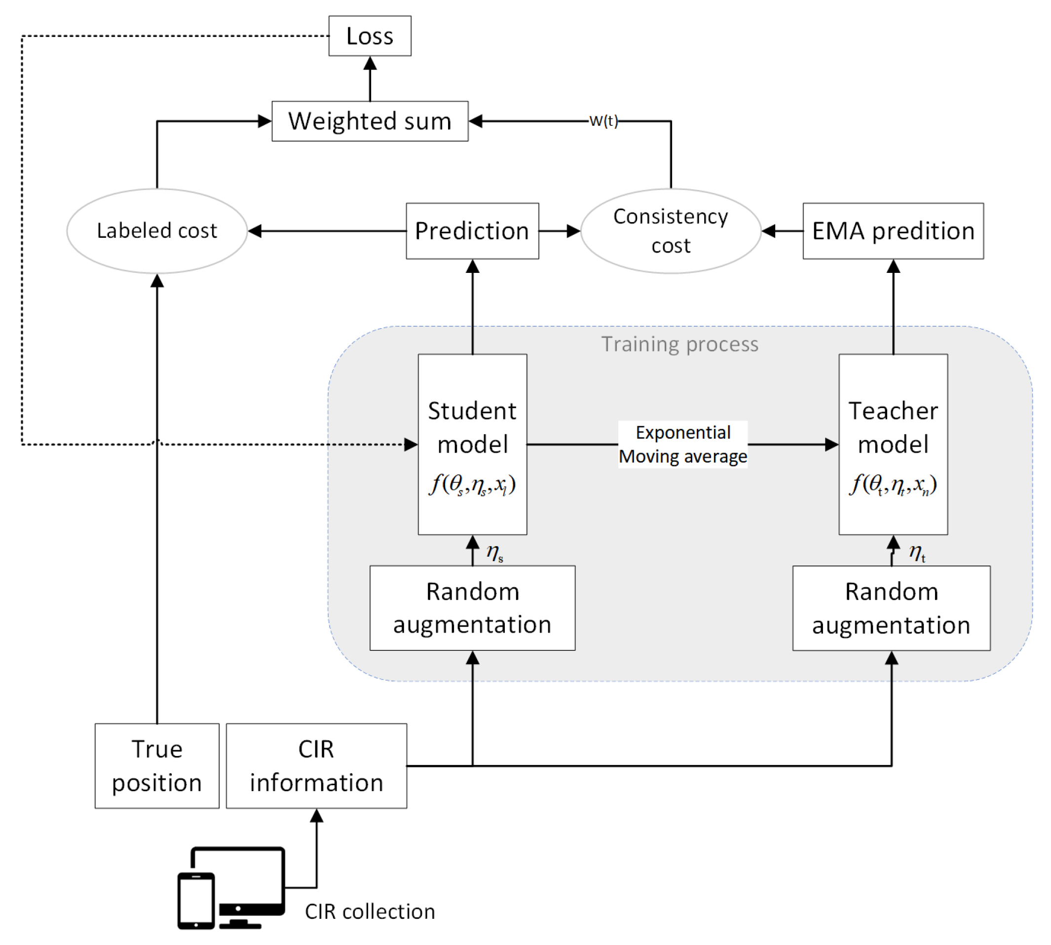
The AMT ensembles the teacher and student model, aiming to train a better teacher model from the student model without additional training. In this paper, the teacher and student models use the same network structure, which can be considered as a self-ensemble method. The framework of the proposed AMT is shown in Figure 2.

Figure 2. The framework of the proposed Adapted Mean Teacher(AMT).

The labeled data are denoted as $X_L={\left\{(x_l,y_l)\right\}}_{l=1}^L$, where L represents the total number of labeled samples. The unlabeled data are expressed as $X_U={\left\{\left(x_u\right)\right\}}_{u=L}^N$, where U represents the total number of unlabeled samples. The total dataset is presented as $X=X_L\cup X_U$, and $X={\left\{x_n\right\}}_{n=1}^N$. The random signal perturbations (data augmentation) for the teacher and student models are denoted as ${\eta }_t$ and ${\eta }_s$, respectively, and the weights of the two neural networks are denoted as ${\theta }_t$ and ${\theta }_s$, respectively. Then, the predictions of the teacher and student models are expressed as $f({\theta }_t,{\eta }_t,x)$ and $f({\theta }_s,{\eta }_s,x)$, respectively, where they use the identical input x with a fixed proportion of labeled and unlabeled data, and both teacher and student models use the same network structure $f(·)$. We first input two CIR data streams, and use different random augmentations for each stream, and then predict UEs’ position using the two models. During training steps, the two models interact, with the teacher model ${\theta }_t^k$ using the EMA weights of the student model. In more detail, at the end of the kth step, the weights of the teacher model ${\theta }_t^k$ are updated using the EMA weights of the student model, and the weight update function of the teacher model is given by

$${\theta }_t^k=\alpha {\theta }_t^{k-1}+(1-\alpha ){\theta }_s^k,$$

(8)

where $\alpha$ represents the smoothing coefficient hyper-parameter.

Instead of regulating the consistency loss of the image classification task in the original Mean Teacher method, we measure the consistency of the users’ predicted coordinates. Therefore, we set the distance function $\mathcal{D}(·)$ as the smooth L1 loss between the batch outputs of data streams instead of the cross-entropy loss. The advantage of using the smooth L1 loss is that the loss can be updated more smoothly, and it is the combination of the L1 and L2 loss with the benefits of both approaches. The specific formula can be expressed as

$$Smooth{L}_1\left(x\right)=\left\{\begin{array}{cc}\hfill 0.5x^2\hfill & \hfill \mathrm{if}\left|x\right|<1\hfill \\ \hfill \left|x\right|-0.5\hfill & \hfill \mathrm{otherwise}\hfill \end{array}\right..$$

(9)

Using the distance Function (9), we define the loss function for the student model, updating in a minibatch as the weighted sum of the labeled loss of the student model and the consistency loss, which is namely the distance between student and teacher model’s prediction. The loss function is

$$\begin{array}{cc}\hfill & \hfill Los{s}_s=\sum _{l=1}^{L}Smooth{L}_1(f({\theta }_s,{\eta }_s,x_l)-y_l)+\hfill \\ & \hfill {ϵ}_{t}w\left({\displaystyle \frac{T}{T_{max}}}\right)\sum _{n=1}^{N}Smooth{L}_1(f({\theta }_t,{\eta }_t,x_n)-f({\theta }_s,{\eta }_s,x_n)),\hfill \end{array}$$

(10)

where $T\in [0,T_{max}]$ represents the current training epoch, $T_{max}$ is a coefficient that represents the maximum ramp-up length, $T/T_{max}$ linearly increases from 0 to 1, and $w(T/T_{max})$ is the unsupervised weight ramp-up function that controls the weight of the unsupervised loss, which increases linearly to 1 over a certain number of epochs. The mild increase in training is important to assist the model in adapting to the increased training interference caused by the unlabeled data and prevent any degradation in performance. In this paper, we use a Gaussian ramp-up function with $w(T/T_{max})=e^{-5{(1-T/T_{max})}^2}$. Additionally, ${ϵ}_t$ is the constant that controls the maximum loss for unsupervised training and is calculated as ${ϵ}_t=w_{max}\times (L/N)$, where $w_{max}$ is a coefficient that represents a maximum weight value for unsupervised training.

At each training step, the student model learns from the teacher model by minimizing the $Los{s}_s$. Through this approach, we can achieve consistency in regularization.

4.2. Data Augmentation

To help models learn abstract patterns in data without being affected by minor changes, the concept of implicit data augmentation has been proposed. The model should tend to provide consistent output for similar data points. In classification tasks, the consistent output refers to the same classification, while in regression tasks, consistent output refers to output vectors that are close in distance. To achieve this goal, minor changes are typically implemented by adding noise or data perturbation. Many regularization techniques rely on this concept, such as the dropout used in neural network models.

In image classification tasks, consistency regularization methods often add random noise to the data in the data augmentation process. Some techniques, such as flipping, resizing, and random cropping can be used to increase the variety of images. The original Mean Teacher method used random translations and horizontal flips as part of its data augmentation strategy [16]. The rationale behind these approaches is that the model’s softmax output usually cannot provide accurate predictions beyond the training data. To alleviate this problem, noise can be added to the model during the inference time to generate more accurate predictions. This method is used in the Pseudo-Ensemble Agreement [48] and has demonstrated excellent performance. Thus, a teacher model injected with noise can be inferred to generate more precise targets than that not injected with noise. Therefore, implicit data augmentation, namely data perturbation, aims to provide accurate predictions by generating new predictions beyond labeled data and adding randomness to prevent overfitting.

4.2.1. Implicit Data Augmentation for CIR

General positioning methods map geometric information to user positions using measurement quantities such as power, time, and angle, then estimate user position through geometric estimation methods. Power, time, and angle features are common physical measurements, each with varying accessibility, complexity, and accuracy. As shown in the estimation of Formulas (2) and (3) for CIR, the three types of information can be well reflected in CIR. Therefore, we infer that power, time, and angle should be extracted as the main useful positioning features as AI positioning methods for using CIR. However, precise angle-based positioning typically relies on the angle difference between multiple antennas on the same device in MIMO communication. In our settings, the number of sampled antennas is insufficient, so we will mainly focus on the power and time of arrival features in AI positioning for using CIR. Inspired by the concept of data augmentation in image classification, we perturb CIR input by adding random noise to critical positioning features, namely the power and time of arrival.

4.2.2. Random Amplitude Scaling

As RSS-based fingerprint positioning systems are commonly used, their fundamental limitation is their inability to capture multipath effects [9]. To fully characterize each path, the wireless communication propagation channel is modeled as a time-linear filter called CIR. CIR is similar to the RSS sequence, but it has a finer frequency resolution and equally higher time resolution to distinguish multipath components. Therefore, we can reasonably infer that CIR has a high power feature for effective positioning, and augmentation can be effectively performed by perturbing the power characteristics of CIR.

The received power measured at a fixed frequency is proportional to the amplitude of the channel frequency response (CFR) [9]. Similarly, in CIR, we infer that the amplitude information is highly relevant to the received power, and different amplitude represents different LOS/NLOS environment distributions. Thus, we propose a random amplitude scaling in training steps to perturb partial LOS/NLOS distribution in the indoor environment, aiming to provide accurate predictions outside the training data. The amplitude of the CIR received by antenna u of UE n from transmitter antenna s can be expressed as:

$$Am{p}^n=\sqrt{Re{\left\{H_{u,s}^n(\tau ,t)\right\}}^2+Im{\left\{H_{u,s}^n(\tau ,t)\right\}}^2}.$$

(11)

The scaling size is represented as a positive random number $\mu$, where $\mu \sim U(0,a)$, with a being the maximum scaling size. Then, the random scaling amplitude can be expressed as $A_{scale}^n=\mu Am{p}^n$. Note that the same scaling on the time series of CIR should be performed to ensure that the shape of the amplitude remains unchanged and to avoid destroying effective positioning features.

4.2.3. Random Temporal Shifting

The time feature is a conventional positioning physical measurement. It can obtain a highly accurate position under LOS conditions. In the positioning situations, there are two conventional time-of-arrival estimation techniques based on CIR; one method is to convert CFR to CIR through the inverse Fourier transform and select the index time of the first peak as the estimated time of arrival. A series of super-resolution techniques are used for estimation; the most commonly used technique is MUSIC algorithm [49]. The other method is based on cross-correlation techniques such as matched filtering [50]. Therefore, we believe that adding perturbations to the time characteristics can randomly shift the overall multipath information of CIR forward or backward, thereby perturbing the index of the first peak. Setting the random perturbation constant as $\lambda$, where $\lambda \sim U(-b,b)$, and for the UE n, the continuous CIR information affected by a delay perturbation can be written as:

$$H_{shift}^n(\tau ,t)=H_{u,s}^n(\tau ,t)\ast \delta (t-\lambda )$$

(12)

where * represents the convolution operation, and $\lambda$ is the translation coefficient with a maximum translation size of b.

5. Convolutional Neural Network for Indoor Positioning

For CIR samples, the structure and dimension of the CIR input are similar to image input, so AI methods used for image processing are considered as our positioning schemes. The most commonly used neural network models for image processing are based on the CNN and self-attention mechanism. Although the concept of deep neural networks is stacking neural networks together, which is observed as a simple process, the performance of these networks can vary greatly due to different network architectures and choices of hyperparameters.

With regard to the models based on CNN, there are several mainstream network structures. AlexNet [51] introduced the concept of deep CNNs and addressed the vanishing gradient problem by utilizing the Rectified Linear Unit (ReLU) activation function while it employed a dropout regularization to prevent overfitting. GoogLeNet [52] further advances the field with its inception module architecture, which allows for the simultaneous use of different-sized convolutional kernels and pooling layers, enabling the extraction of features at multiple scales. On the other hand, ResNet [53] introduces the concept of residual learning. It addresses the degradation problem that arises when deep neural networks suffer from a diminishing performance with increasing depth. By employing skip connections, ResNet allows for the direct flow of input to the output layer, facilitating the learning of residual mappings.

The self-attention mechanism [54] focuses on the correlation of vectors in input sequences, and it was first used for semantic comprehension. When applying the self-attention to image processing tasks, images are divided into small parts and input as sequences. The most typically used model is the Vision Transformer (ViT) [55]. ViT is an effective tool for handling large images and complex visual scenes. This model can also enhance its performance through pre-training.

To effectively extract features for positioning, we consider a ResNet structure as the basic model for AMT. It is applied in both student and teacher models. The ResNet has several advantages, including its extremely deep network structure, which enhances the network’s ability for feature extraction. Additionally, it introduces the residual blocks, which prevent network degradation, gradient vanishing, or gradient explosion in deeper networks.

5.1. Residual Network

ResNet features two main types of residual blocks: the basic block and the bottleneck block. The basic block consists of two 3 × 3 convolutional layers and a residual connection with a stride of 1, while the bottleneck block includes a 1 × 1 convolutional layer, a 3 × 3 convolutional layer, another 1 × 1 convolutional layer, and a residual connection. The 1 × 1 convolutional layer in the bottleneck block is primarily used to decrease the dimension of the feature map, thereby reducing the computation and parameter count.

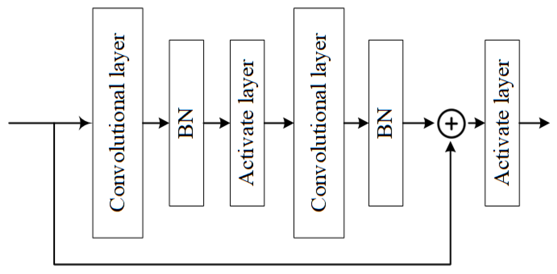
In this paper, we consider a basic block of residual blocks. The structure of residual blocks is shown in Figure 3. The core of ResNet’s residual blocks lies in its residual connection, which adds the output of the previous layer to the current layer’s output, enabling the current layer to incorporate information from the previous layer. This design effectively alleviates the problem of gradients vanishing, making the model easier to train and optimize.

Figure 3. Structure of a residual block.

The ResNet consists of residual blocks that are based on the convolutional layer. For the purpose of accelerating the model convergence speed and improving model performance, we added BN and activation function layers between convolutional layers in the residual structure of ResNet. The Batch Normalization (BN) layer normalizes the input of each layer in a deep neural network for each batch, which stabilizes the input distribution of each layer and accelerates model convergence speed. Assuming the input after augmentation is x, for a layer with multiple input dimensions, the BN operation [56] for each dimension can be expressed as:

$$\widehat{x}={\displaystyle \frac{x-E\left(x\right)}{\sqrt{Var\left(x\right)}+\epsilon }}$$

(13)

where $E\left(x\right)$ and $\sqrt{Var\left(x\right)}$ present the expectation and variance of the input mini-batch respectively, and $\epsilon$ is a small coefficient to prevent the denominator from being zero, which approximates to 0.

Alternatively, the activation function layer, ReLU function, is used in the structure due to its simplicity and non-linearity. This function is added after the BN operation to effectively mitigate the gradient vanishing problem and enhances the model’s performance. The activation function can be mathematically presented as

$$\sigma (·)=ReLU\left(\widehat{x}\right)=max(\widehat{x},0),$$

(14)

5.2. CNN-Based Regression Positioning Method

In the previous research about classification-based fingerprint positioning, the area was divided into small grids, and the fingerprints were mapped to the reference point (RP) in the grid [57,58]; however, this approach is not suitable for large areas because of the extensive number of classes it needs to be divided into, and this will greatly increase the model complexity in deep learning-based fingerprint positioning. Meanwhile, a straightforward classification method of fingerprint positioning first defines RPs by collecting features at different points and then finding the similarity between the target feature and different RPs. This heavily depends on the number and density of RPs because of the limited training space; it is hard to reach sub-meter level accuracy in large areas. In contrast, the regression method can overcome the discontinuity of RPs and has the potential to reach higher accuracy, while it is also insensitive to the size of areas. From these concerns, we use the regression method rather than the classification.

6. Simulations

In this section, we conduct simulation experiments based on the open-source dataset in order to evaluate the positioning performance of our proposed method.

6.1. Simulation Settings

3GPP Technical Report 38.901 [47] has outlined an indoor factory with dense clutter and a high base station height (InF-DH) scenario with its lower probability of LOS conditions. We evaluate the performance of our proposed AMT method based on the InF-DH scenario specified by 3GPP.

The indoor factory scenario is a highly intricate industrial environment characterized by obstacles. As shown in Figure 4, 18 BSs are deployed on the ceiling of the factory with a length of 120 m and a width of 60 m. The clutters in the scene can be considered as machinery, assembly lines, and storage shelves, and UEs are uniformly distributed in the area.

Figure 4. Indoor positioning scenario.

We use an open-source indoor measurement dataset WLI_3_ 1015_InF_DH662_FR1 _drop1_ cir_ rsrp _toa_tdoa from [59], the full parameter settings of the dataset simulation can be found in the introduction_positioning file, and we list partial parameter setting of system-level simulation in Table 1. The dataset generated by the system-level simulator is generated according to the 5G-NR standard of 3GPP [47]. In the system-level simulation, the clutter’s density, height, and diameter are 60%, 6 m, and 2 m, respectively, which are used to generate a heavy NLOS indoor scenario. The BS antenna configuration is denoted by ($M^a$, $N^a$, P, $M_g^a$, $N_g^a$), and $M^a$ and $N^a$ indicate that a single panel array antenna has an $M^a$×$N^a$ uniform planar array, where $N^a$ is the antenna in each row and $M^a$ is the number of rows in the vertical dimension. P represents the number of polarization dimensions, $M_g^a$ and $N_g^a$ illustrate that the antenna system consists of $M_g^a$ vertical panels and $N_g^a$ horizontal panels, and in the parameter setting, we only use one antenna in the receiver/UE side. Spatial consistency is used to keep the various channel generation steps spatially consistent for a drop-based simulation, and this process is not used in the simulator. The UE is moving in a random direction with a fixed speed of 3 km/h, which means the orientation of the antenna is random.

Table 1. Parameter settings for generating datasets.

Parameters	Values
Clutter density, height, size	0.6, 6 m, 2 m
Bandwidth	100 M
TX power of total base station(BS)	24 dBm
BS antenna configuration	($M^a$, $N^a$, P, $M_g^a$, $N_g^a$) = (4, 4, 2, 1, 1)
Antenna height of user equipment(UE)	1.5 m
BS height	8 m
Carrier frequency	3.5 GHz
Subcarrier spacing	30 kHz for 100 MHz
Spatial Consistency	No
Synchronization between BS and UE	Ideal
Penetration loss	0 dB
Number of floors	1
UE mobility	3 km/h
Min BS-UE distance (two dimensional)	0 m

From the settings of the system-level simulation, we can infer that there may exist some errors in AOA because of the randomness of UEs’ orientation. These errors will directly affect the phase of CIR by introducing errors in field patterns, which will influence the measurement of AOA. However, because the useful angle information for the position estimation contained in CIR exits in the angle difference between antennas and we only use one antenna for receiving signals, it will not result in many errors in our positioning scheme. However, when facing the effects of antenna orientation, improvements in the estimation method of AoA can help increase the estimation accuracy of AoA [60], and using machine learning methods to assist position calculation using AoA estimation can also help enhance the positioning accuracy [61]. Also, the number of antennas is proven to affect the positioning performance by improving the resolution in AoA estimation [62]; therefore, in practical situations, the user devices with more antennas will also benefit the positioning performance.

We sample CIR data by truncating the first 256 time-domain points based on the first Tx antenna element and the first Rx antenna element from CIR, and the corresponding multipath characteristic of CIR is represented in Figure 5. In the dataset, the CIR received by each UE is represented as a three-dimensional vector of “$18\times 256\times 2$”, which represents the UE received CIRs from 18 BSs, and each CIR contains 256 complex-valued sampling points.

Figure 5. The received channel impulse response(CIR) of a UE from a single BS.

The dataset consists of 80,000 CIRs corresponding to true UE coordinates. A total of 78,400 data samples are used as the training set while 1600 are used for a test set. Ignoring the inter-UE correlation changes caused by the reduction in the number of UEs, we randomly select 3000 or fewer UEs from the training set as labeled data to simulate the limited labeled data scenario for indoor positioning. We assign a label of 0 to the remaining data, treating them as unlabeled data. The student and teacher models are trained with a fixed ratio of 1:1 for unlabeled and labeled data. To maintain the fixed ratio of labeled and unlabeled data, a two-stream batch sampler is used to obtain a training batch, and a batch size of 256 is used for each stream. In the augmentation process, we select 5% of labeled data samples to operate amplitude scaling or temporal shifting and set the maximum scaling size a as 3 while the maximum translation size b is set to 5. We should keep the perturbed data as a small portion of the labeled data to ensure that critical positioning features are not completely destroyed. It should be noted that the perturbation here should operate in the training steps of each mini-batch instead of scaling the amplitude for the overall data first. For the reason that a large learning rate is prone to causing non-convergence or a gradient explosion phenomenon in the simulation, we carefully select an optimizer and a small learning rate.

For the parameter setting of AMT, we set the ramp-up length $T_{max}$ to 80, which means that $w(T/T_{max})$ linearly increases to 1 within 80 epochs. To prevent training from degrading, $w(T/T_{max})$ is set to 0 when the epoch starts from 0. We set the maximum value of the unsupervised weight $w_{max}$ to 70. In addition, the smoothing coefficient $\alpha$ of EMA is fixed at 0.97. The value of $\alpha$ is set to ensure that the teacher model keeps up with the rapidly evolving student model by promptly disregarding erroneous prior values of the student model. The performance of the teacher model is considered to be the final result. The detailed parameter settings of AMT are concluded in Table 2.

Table 2. Parameter settings for AMT training.

Parameters	Values
Number of samples	80,000
Number of samples for training	78,400
Number of samples for testing	1600
Network structure $f(·)$	Resnet
Batch sampler	Two-stream batch sampler
Batch size	512 (256 for each stream)
$w_{max}$	80
$T_{max}$	80
$\alpha$	0.97
Training epoch	200
Optimizer	Stochastic Gradient Descent
Learning rate	0.001
Perturbed proportion of labeled data	5%

In our simulation experiments, positioning accuracy and convergence are used as the performance metrics of the proposed AMT model. In particular, we adopt 90%, 80%, 67%, and 50% points of the Cumulative Distribution Function (CDF) of the positioning accuracy to illustrate the performance gain in accordance with the evaluation methodology in 3GPP TR38.857.

6.2. The ResNet Model for Processing CIR

For the model basic structure $f(·)$, we design a ResNet to extract effective positioning features from CIR information, which is originally used for processing multi-channel image information in the field of image processing [53].

A ResNet structure for feature extraction is shown in Figure 6. It consists of four reshape layers and six residual blocks, while the reshape operation serves to preprocess the data and adapt it to the input dimension of the residual block.

Figure 6. Structure of Resnet.

Specifically, in the design, the input data dimension is considered as a 2-channel image data of size 18 × 256. In the first four layers of the network, the dimension of the input information increases to 18 × 18 with 64 channels so that it is able to be processed by 3 × 3 convolutional kernels in the residual blocks. Then, the residual blocks are used for training, with the input being directly added to the output of a residual block, which is known as a shortcut connection. In terms of a shortcut operation, when a dimension change occurs between residual blocks, the input propagation between blocks needs to be dimensionally changed to adapt to the next residual block. This procedure is marked by the dotted line in Figure 6. After the pooling layer, a linear layer with an output dimension of two is used to obtain the UE’s two-dimensional coordinates.

6.3. Results and Discussions

6.3.1. Performance Evaluation of the Supervised Learning-Based Method

Before conducting the simulation of the semi-supervised and enhanced indoor positioning under limited labels, we first evaluate the performance of positioning under a supervised learning situation, which uses the full labels in the fingerprint dataset and an original CIR input without augmentation. For an objective comparison, we also use other fingerprinting methods based on deep learning and a traditional estimation method to test their positioning accuracy under the heavy NLOS scenario.

The full number of labeled data for input is 80,000. In the supervised learning trial, we also use the rate of 2% to divide the training set and test set. In CIR-based fingerprint indoor positioning, we use the ResNet structure mentioned in 5.1 to conduct the simulation. In the training process, the batch size and learning rate are set to 512 and 0.1 respectively; the adam optimizer and cosine-annealing scheduler are also used in the training.

Meanwhile, we also process the TOA, TDOA, and RSS fingerprints that are collected in the same scenario with the same collecting steps to deal with the positioning task using a learning-based method. The structure of a single datum is 1 × 18, which stands for the TOA/TDOA/RSS signal received from 18 BSs. These fingerprint datasets are also listed in WLI_3_1015_InF_DH662_FR1_drop1_ cir_rsrp_toa _tdoa from [59]. To avoid destroying the dimension of these fingerprints, we applied a Multi-layer Perception(MLP) network to recognize the features. The MLP structure consists of 4 linear layers with an activation function ReLU connected to each linear layer and a dropout operation before the last linear layer.

Additionally, we also apply CHAN, a traditional method that is widely used in TDOA-based positioning [21]. By utilizing the TDOA fingerprint values and the known BS positions to apply the Weighted Least Squares (WLS) algorithm, we can obtain the calculated position of UEs, noting that the algorithm is under the case of more than three reference nodes.

The position performance can be reflected by the CDF of positioning errors and Mean Error (ME), which are shown in Table 3. By comparing the performance of the learning-based fingerprint positioning and CHAN, we can conclude that AI positioning methods are superior to the traditional TDOA-based estimation algorithm. In the performance of learning-based fingerprint positioning, all displayed methods reach the accuracy of sub-meter level, while the CIR-based method has the best positioning accuracy, which reaches an ME of 0.31 m.

Table 3. Comparison of position accuracy based on supervised learning.

Method for Indoor Positioning Using Deep Learning	CDF Percentile of Position Errors (m)				ME (m)
	50%	67%	80%	90%
CIR-based fingerprint positioning	0.28	0.35	0.45	0.54	0.31
TOA-based fingerprint positioning	0.36	0.46	0.57	0.69	0.40
TDOA-based fingerprint positioning	0.38	0.49	0.60	0.74	0.41
RSS-based fingerprint positioning	0.30	0.41	0.52	0.68	0.38
CHAN	10.35	16.01	22.08	31.14	14.72

After the performance evaluation of CIR-based fingerprint positioning, we can observe that it outperforms positioning methods based on other measurements collected from the same scenario; thus, it is more effective to use it as the basic module in our proposed training framework.

6.3.2. Numerical Results of Semi-Supervised Learning-Based Method

In this simulation, we conducted tests with a very small sample size, specifically using 3000 or fewer samples to evaluate the performance.

On the basis of supervised learning, we first verified the effectiveness of the proposed data augmentation methods. From Figure 7, it can be observed from four performance curves with different numbers of labels that the number of samples is positively correlated with the positioning accuracy. Additionally, from the comparison of Figure 7a–c, it is clear that both proposed data augmentation methods can effectively improve the positioning accuracy for all test samples in supervised learning (SL) methods, with the most significant improvement observed for sample sizes ranging from 500 to 2000. This demonstrates that our proposed data augmentation methods can adapt to scenarios with very few labeled data and meet practical needs. In terms of the effectiveness of the two data augmentation methods, amplitude scaling is significantly better than temporal shifting when the number of labels is 500, and it also performs slightly better than the temporal shifting for other sample sizes.

Figure 7. Supervised positioning performance under different samples and augmentation methods. (a) Performance of supervised learning(SL) method only. (b) Performance of SL method with temporal-shifting augmentation. (c) Performance of SL method with amplitude-scaling augmentation.

To judge whether the unlabeled data are effective for a performance improvement in DSSL methods, we obtain the positioning accuracy of AMT to compare with the performance of purely supervised learning using a few labeled data to train the model. After verifying the effectiveness of two data augmentation methods in the SL method, we conduct the AMT model by using the two proposed augmentation methods. By comparing Figure 8a,b to Figure 7b,c), we observe that the performance of AMT significantly improves in four cases compared to purely supervised learning methods, while it applies two proposed data augmentation techniques. Additionally, similar to purely supervised learning, the use of the random amplitude scaling augmentation method attains better performances than random temporal shifting in four cases. Furthermore, the AMT method in the case of small sample sizes demonstrates more significant improvement, specifically when the number of labeled samples is less than 2000. A visualization example to show the performance of AMT using 1000 labeled samples is present in Figure 9.

Figure 8. Performance of AMT with different augmentations. (a) Performance of AMT with temporal-shifting augmentation. (b) Performance of AMT with amplitude-scaling augmentation.

Figure 9. A visualization form to show the distribution of UEs. The red dots represent the actual user locations, while the blue dots represent the predicted user locations.

Furthermore, we verify the effectiveness of the proposed AMT model by comparing it with several reference algorithms under 1000 labeled samples. In order to facilitate better horizontal comparison, we will use some DSSL methods that have similar training frameworks and steps to AMT as benchmark algorithms. One reference algorithm is the $\mathrm{\Pi }$ Model and the other is the Temporal Ensembling. Both two algorithms are advanced consistency regularization methods, and the same data augmentations are used for the three approaches. In addition, we also compare the performance of the pseudo label to verify the effectiveness of our method because it is widely used for positioning. As numerical results are shown in Table 4, we can observe that the three consistency regularization methods significantly outperform the pseudo label in positioning accuracy. Moreover, among the three consistency regularization methods, the AMT model achieves the highest accuracy. Meanwhile, we compare the convergence of the four methods and record the tendency of the positioning error corresponding to 90 percentile CDF. During the training process, we can observe from Figure 10 that although there is a small difference in the positioning error of AMT, $\mathrm{\Pi }$ Model and Temporal Ensembling, the convergence of AMT is significantly faster than the other two methods, while the convergence curve seems to be smoother. This implies that under the condition of limited training time, the AMT model demonstrates obvious advantages over the other two referenced consistency regularization methods.

Table 4. Comparison of position accuracy under 1000 labeled samples.

DSSL Method for Indoor Positioning	CDF Percentile of Position Errors (m)				ME(m)
	50%	67%	80%	90%
Proposed AMT with amplitude scaling	0.79	1.03	1.27	1.63	0.90
Proposed AMT with temporal shifting	1.18	1.53	1.85	2.27	1.29
Temporal Ensembling with amplitude scaling	0.82	1.06	1.33	1.65	0.93
Temporal Ensembling with temporal shifting	1.20	1.54	1.88	2.33	1.31
$\mathrm{\Pi }$ Model with amplitude scaling	0.84	1.10	1.36	1.74	0.96
$\mathrm{\Pi }$ Model with temporal shifting	1.20	1.54	1.89	2.33	1.32
Pseudo label	1.45	1.87	2.29	2.93	1.65
Supervised only	1.71	2.19	2.76	3.33	1.91

Figure 10. Tendency of position errors.

During the training process, we also recorded the tendency of positioning error in Figure 11. The utilization of AMT can be understood through the training curves. The models with EMA weighting (represented by the orange curves in the bottom row) exhibit more accurate predictions compared to the student models (represented by the blue curves) after an initial period.

Figure 11. Positioning errors of teacher and student models under 1000 labeled samples.

When the EMA-weighted model is employed by the teacher, it leads to enhanced outcomes in semi-supervised scenarios. A virtuous feedback cycle appears where the teacher model (orange curve) improves the student model (blue curve) through the application of consistency cost. Simultaneously, the student model contributes to the improvement of the teacher model via EMA.

6.3.3. Discussions

To analyze the performance differences between random amplitude scaling and random temporal shifting, the amplitude scaling technique performs better than temporal shifting. In this paper, we consider several possible reasons. First, time-based ranging typically uses an external signal source and heavily relies on complex signal processing methods, which means it generally relies on super-resolution methods like the MUSIC algorithm to obtain the first arrival peak as an arrival time. However, in our CIR training sets, CIR information is not continuous; it is selected as time intervals, which makes the time sequence discrete. This decreases the resolution of the time sequence in CIR and possibly leads to an incorrect recognition for the model. The power-based features vary over time, but the shape of the peak does not change rapidly between a few sampling points. Moreover, the entire CIRs’ peaks can be utilized to estimate the location, rather than solely relying on the arrival time of the first peak. This may be a reason why the power-based feature is more effective than the time-based feature, and power scaling exhibits a better performance in augmentation. Meanwhile, the time-based ranging relies highly on the LOS condition, a positive bias could be induced in NLOS propagation and a larger variance tends to exist in the NLOS condition [63].

To analyze the performance of methods in Table 4, we re-examine the fundamental principles of these four methods. The $\mathrm{\Pi }$ Model and Temporal Ensembling only use a consistency loss for learning while the AMT uses both the weights of the student model and consistency loss for learning. Interactions in weights can help learn the performance of supervised training rapidly from the beginning instead of receiving feedback at the end of each epoch to punish inconsistent items, which greatly reduces time costs. Similarly, like AMT, the pseudo label also uses the training weights of supervised training, manifesting as no significant positioning error at the beginning of training. However, due to the small amount and sparse distribution of labeled data, the pseudo-label method cannot learn information beyond this sparse distribution, which leads to a limited performance during training with dense but unlabeled data, and results in a relatively low positioning accuracy.

7. Conclusions

In this paper, we proposed an effective DSSL framework for InF-DH scenarios named AMT, which solves the problem of inaccurate positioning caused by inadequately labeled samples for fingerprint positioning. In the DSSL framework, we operate AMT by assigning the EMA weights of the student model to the teacher model and regularizing the consistency loss of two models. Additionally, we have also proposed novel implicit random augmentation methods in terms of amplitude and temporal features of CIR data in AMT to enhance the performance of neural networks. By adding random perturbation to these critical positioning features in the training process, continuous new data can be generated artificially from existing data.

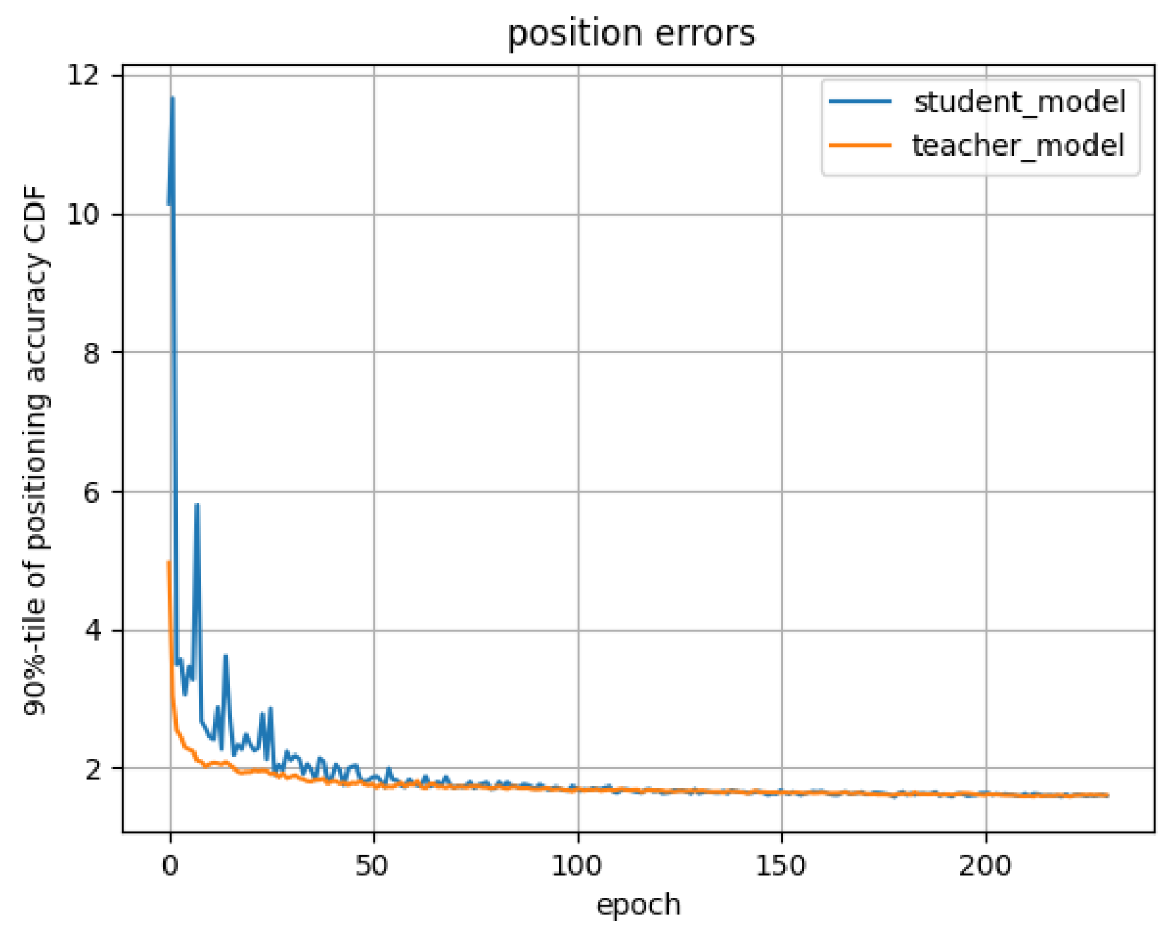
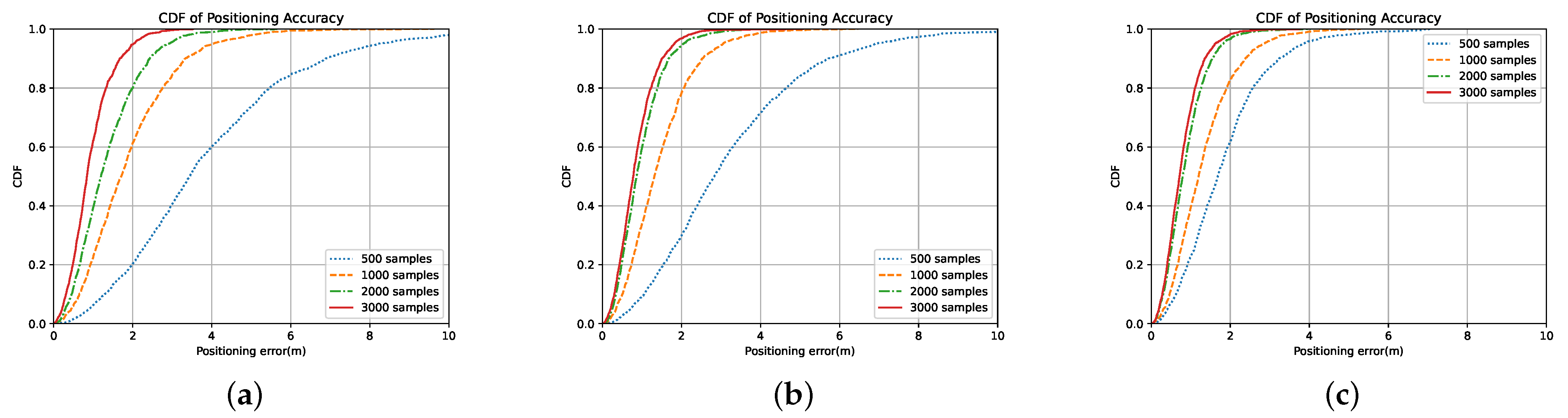
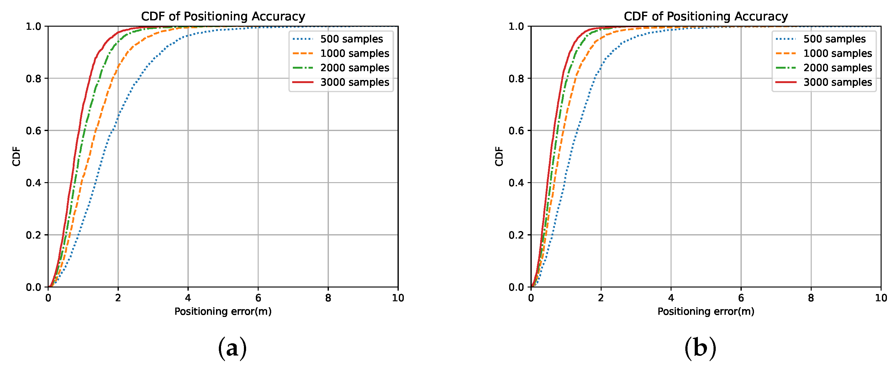
From conducting the simulation, we conclude that the deep-learning method has a superior performance compared with the estimation method in the heavy NLOS scenario, which can achieve a sub-meter level accuracy, and using CIR for deep learning-based positioning can achieve a higher positioning accuracy than using other measurements proposed in the 5G NR standard. By analyzing the performances of the DSSL methods, the numerical results show that using regularization in consistency loss improves the neural network’s ability to resist perturbation, which helps learn effective features in unlabeled data, especially in the case of small samples. Meanwhile, the interaction in model weights for consistency regularization methods improves the convergence of neural networks. Additionally, results also show the robustness of AMT by using different numbers of labeled data, and its performance gain in the smaller samples is more obvious.

By using AMT, we find the inherent similarity between image processing and indoor positioning, and we also verify the effectiveness of image processing methods when applying them to the positioning field. However, the work does not involve using the angle feature for positioning because of the single receiving antenna set in the dataset. Since multiple receiving antennas can bring more channel information for positioning, we plan to explore the generalization of our proposed method in multiple-receiver situations in future studies.