Large-Scale Subspace Clustering Based on Purity Kernel Tensor Learning

Abstract

In conventional subspace clustering methods, affinity matrix learning and spectral clustering algorithms are widely used for clustering tasks. However, these steps face issues, including high time consumption and spatial complexity, making large-scale subspace clustering (LS${}^2$C) tasks challenging to execute effectively. To address these issues, we propose a large-scale subspace clustering method based on pure kernel tensor learning (PKTLS${}^2$C). Specifically, we design a pure kernel tensor learning (PKT) method to acquire as much data feature information as possible while ensuring model robustness. Next, we extract a small sample dataset from the original data and use PKT to learn its affinity matrix while simultaneously training a deep encoder. Finally, we apply the trained deep encoder to the original large-scale dataset to quickly obtain its projection sparse coding representation and perform clustering. Through extensive experiments on large-scale real datasets, we demonstrate that the PKTLS${}^2$C method outperforms existing LS${}^2$C methods in clustering performance.

1. Introduction

Clustering is a method that groups data with similar features into the same category, showing the dissimilarity between clusters and the similarity within clusters. It has been widely used in the field of data analysis [1]. However, traditional methods (such as K-means [2]) cannot inefficiently cluster high-dimensional data, because of the complex structures [3]. Since the effective information in high-dimensional data usually resides in low-dimensional structures, many subspace clustering methods have been proposed. These subspace-based clustering methods have proven to be effective in mining feature information from high-dimensional data and are widely applied in handling computer vision tasks [4,5].

Classic subspace clustering methods typically rely on the self-representation (SE) property of the data, i.e., any data point within the same subspace can be represented as a linear combination of other distinct data points [6]. The goal is to find the minimal number of $base$ $points$, such that all other points are linear combinations of the $base$ $points$. This can be expressed by the following formula:

$$\begin{array}{c}\hfill \underset{\mathit{C}}{min}rank\left[\frac{1}{2}{\parallel \mathit{X}-\mathit{X}\mathit{C}\parallel }_F^2+\lambda \Re \left(\mathit{C}\right)\right]\mathrm{s}.\mathrm{t}.\mathit{C}⩾0,\end{array}$$

(1)

where $\mathit{X}$ is the input data, $\lambda >0$ is a regularization parameter, $\mathit{C}$ is the SE coefficient matrix, and $\Re \left(\mathit{C}\right)$ is the regularization term. In these methods, the affinity matrix is obtained by applying different norms to the square of $\Re \left(\mathit{C}\right)$ and different algorithms in different scenarios. Finally, spectral clustering [7] is used to segment the affinity matrix and obtain the final clustering results [8].

However, with the continuous increase of the data scale, complex negative factors (including noise, data missing, etc.) and nonlinear structures in large-scale data seriously degrade the accuracy and increase the computational complexity of clustering tasks. Consequently, traditional subspace clustering methods (such as SSC [9], LRR [10], and LSR [11]) are not applicable to large-scale data clustering. This is because—when applying these methods to large-scale data—they will inevitably encounter large-scale SE matrices and encode models [12,13,14]. Meanwhile, spectral clustering algorithms also have high computational complexity ($O\left(n^3\right)$, n is the number of samples) [15] and large memory usage. Therefore, it is necessary to explore subspace clustering methods that are applicable to large-scale data.

To overcome this problem, the current mainstream approaches involve extracting a small set of data from the large-scale raw data based on the self-representation property, to perform subspace clustering tasks and then extend them to the raw data [16]. Although this method shows its success in performing LS${}^2$C tasks, there are still some issues that need to be addressed: (1) performing a simple sparse representation or low-rank representation of the sampled data leads to the limited acquisition of sample feature information, resulting in evident errors when predicting the feature information of the original large-scale data [17,18] in many cases; (2) real data points are usually distributed in several nonlinear subspaces, and the above methods cannot effectively handle the nonlinear structure of the data; (3) only applying simple constraints (e.g., $l_{2,1}$ norm, F-norm) to the noise in the sample data will seriously degrade the clustering accuracy.

Toward the challenges mentioned above, we designed a novel LS${}^2$C method: pure kernel tensor learning-based large-scale subspace clustering (abbr. PKTLS${}^2$C). Mainly three techniques are proposed in PKTLS${}^2$C. Firstly, PKTLS${}^2$C extracts a small set of samples from the original dataset, uses kernel tricks to map the sample dataset to a high-dimensional Hilbert space, and stacks the resulting kernel matrices to form a third-order tensor. This leads to the effective handling of nonlinear structures while acquiring more feature information, which is beneficial for reducing errors in predicting the feature information of the original data. Secondly, PKTLS${}^2$C separates the noise information from the kernel tensor, retains the main information, updates the self-representation matrix of the sample dataset, and applies $l_{2,1}$ norm constraints to the self-representation matrix. So, PKTLS${}^2$C ensures the sparse low-rank properties while avoiding the influence of specific data errors [19]. This denoising method can effectively enhance the robustness of the model and improve clustering performance. Finally, a deep autoencoder is designed for PKTLS${}^2$C, which is trained with the learned self-representation matrix of the sample dataset. When the training was complete, we applied the autoencoder to the original large-scale dataset to project and obtain its feature representation, thereby achieving the goal of reducing computational complexity. Figure 1 shows the main structure of PKTLS${}^2$C. The main contributions of this paper can be summarized as follows:

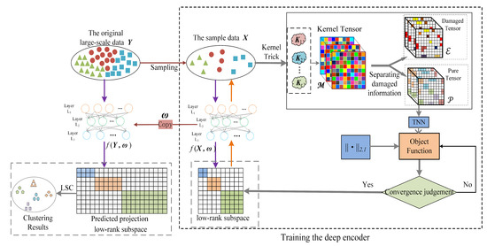
Figure 1. Schematic diagram of the PKTLS${}^2$C structure.

• We propose a secondary denoising method to process the sample dataset, providing cleaner training samples for the deep encoder to predict the feature information of the original dataset.
• By ingeniously integrating multi-kernel learning and tensor learning, and applying it to large-scale dataset subspace clustering tasks, we can delve more deeply into sample feature information and effectively handle the nonlinear structures. This approach significantly reduces the prediction error of feature information for large-scale datasets.
• We designed a learnable deep encoder with multiple hidden layers that can effectively manage the nonlinear structures in large-scale datasets and obtain the feature representation of these datasets by projection.
• We integrate ADMM and GD into PKTLS${}^2$C and design an optimization method. We validate the advantages of PKTLS${}^2$C to the existing approaches via experiments with datasets consisting of millions of samples.

2. Related Work

In this section, we mainly review the existing approaches to large-scale spectral clustering, scalable subspace clustering, and autoencoder-based subspace clustering, and summarize the strategies dealing with the LS${}^2$C problem.

2.1. Large-Scale Spectral Clustering

Spectral clustering involves calculating the eigenvectors of the affinity matrix generated by the model and then using K-means to cluster these eigenvectors [7]. However, computing the feature vector involves high computational complexity and large memory usage [20]. Therefore, it is very difficult to apply spectral clustering methods to perform subspace clustering tasks on large-scale datasets [21]. In order to extend the spectral clustering method to large-scale datasets, Nystr$\ddot{\mathrm{o}}$m [22] uses approximate eigenvectors of the affinity matrix to calculate the required eigenvalues in multiple subsystems at the same time [21], speeding up the computation process and meeting the requirement of large memory usage. Other approaches [1,23,24] sample a small subset of data points from the original dataset as landmarks, construct the affinity matrix from this sampled dataset, use spectral clustering to determine the feature space of the sampled dataset, and finally employ K-means or other methods to categorize the remaining data into their respective subspaces. However, due to the complex structures of the datasets, the constructed affinity matrix cannot effectively divide the subspace, degrading the clustering performance. In contrast, PKTLS${}^2$C can effectively deal with the complex structure of datasets and improve the accuracy of clustering.

2.2. Scalable Subspace Clustering

Scalable subspace clustering is a commonly used method to handle LS${}^2$C. It involves sampling a small set of data points and initially performing clustering on this sample dataset to reduce computational complexity.

SSSC [1] firstly samples from a large-scale dataset, then classifies the sample dataset, and finally uses the sparse-representation-based classifier (SRC) [25] to assign the out-of-sample data to the divided subspace. Similarly, the sampling–clustering–classification method [14] also processes large-scale datasets by first clustering the sample dataset and then using a linear classifier. Unfortunately, these two methods still require considerable time to process large-scale datasets and often result in poor clustering accuracy, as the simple classifier cannot effectively identify complex out-of-sample data. You et al. proposed ENSC [26], which reduces computation time by finding the optimal coefficients between sample data and out-of-sample data, processing only the sample dataset. You et al. also proposed ESC [27] using a distance-first search algorithm to find a representative subset to represent all data points. Kang et al. proposed SGL [28] using the idea of anchors to sample data as landmarks and employing K-means to partition all the data points into the subspace determined by the sample dataset. These methods select a small set of sample data to represent all the data points based on the SE property of the data to reduce computational costs. However, they cannot guarantee clustering accuracy due to the complex structure of the out-of-sample data points. Compared to these methods, PKTLS${}^2$C can quickly calculate the representation matrix of the out-of-sample data and ensure its robustness.

2.3. Autoencoder-Based Subspace Clustering

PKTLS${}^2$C uses a learned deep encoder to calculate the sparse representation of all data points, thereby reducing computational complexity. An autoencoder is commonly used by the existing methods. However, it still faces some challenges. For example, an autoencoder (AE) [29] or a sparse autoencoder (SAE) [30] just encodes the data directly and cannot deal with the noise in the dataset. Although the denoising autoencoder (DAE) [31] can output robust coded representation, it does not have the ability to directly deal with the noise existing in the dataset. The RPCA encoder (RPCAec) [32] outputs a robust encoded representation by separating the noise from the dataset, but it only encodes for a single subspace in each round of execution. In contrast, PKTLS${}^2$C ensures the purity of the input dataset and the robustness of the model by means of secondary denoising. So, PKTLS${}^2$C can output the coded representations of multiple subspaces at the same time.

3. PKTLS${}^2$C Model

In this section, we first explain the notations used in this paper, then introduce how to train the autoencoder and process the sample dataset. Finally, we analyze the optimization scheme and the computational complexity of PKTLS${}^2$C in detail.

3.1. Notations

To standardize the use of notations, a tensor is denoted by a calligraphic capital letter, e.g., $\mathcal{P}$, and a matrix is denoted by a bold capital letter, e.g., $\mathit{C}$. Table 1 summarizes the meaning of the symbols used in this paper.

Table 1. Meaning of notations used in the text.

Notations	Meaning
$\mathit{Y}$	Original dataset
$\mathit{X}$	Sampled dataset
$\omega$	Parameters learned by the deep encoder
$\mathcal{M}$	Constructed kernel tensor
$\mathcal{P}$	The pure kernel tensor
$\mathcal{E}$	The damaged kernel tensor
${\mathit{K}}^{\left(i\right)}$	The i-th kernel Gram matrix
$\mathit{C}$	Sampled data self-representation matrix
$f(·,\omega )$	Deep encoder
$Tr(·)$	The trace operator of a matrix

3.2. Design of the Deep Self-Encoder

To efficiently solve the complex computational problem in the LS${}^2$C process, learned coordinate descent (LCoD) [33] can learn a sparse-coded representation of the original data by training a feed-forward neural network. Based on this idea, we designed a non-iterative deep encoder to learn the low-rank sparse representation of the original data for reducing the high computational complexity. It can be represented by the following mathematical form:

$$\begin{array}{c}\hfill \mathit{C}=f(\mathit{X},\omega ),\mathrm{s}.\mathrm{t}.\mathit{X}=\mathit{X}\mathit{C},\end{array}$$

(2)

where $\mathit{X}=[{\mathit{X}}_1,{\mathit{X}}_2,\dots ,{\mathit{X}}_m]$ is the input data, $\mathit{C}$ is the representation coefficient, and $\omega$ is the parameter learned by the deep encoder. During the process of training the deep encoder, we use gradient descent (GD) [34] to minimize the loss function $\mathcal{L}\left(\omega \right)$, which can be defined as

$$\begin{array}{c}\hfill \mathcal{L}\left(\omega \right)=\frac{1}{m}\sum _{i=1}^{m}L\left({\mathit{X}}_i,\omega \right).\end{array}$$

(3)

From Equation (3), we cannot compute the expectation error directly, because we do not know which ${\mathit{X}}_i$ in $\mathit{X}$ is a noise point. Fortunately, we can take advantage of the SE property of the data and use $\mathit{X}$ as an SE dictionary, which can solve the problem of generating a trivial solution during the encoding of the predicted computational data. So, we can consider the squared error function and obtain the following form:

$$\begin{array}{c}\hfill \mathcal{L}\left(\omega ,{\mathit{X}}_i\right)=\frac{1}{2}{∥{\mathit{C}}_i-f\left({\mathit{X}}_i,\omega \right)∥}^2,\mathrm{s}.\mathrm{t}.\mathit{X}=\mathit{X}\mathit{C}\end{array}$$

(4)

for $1\le i\le m$, where ${\mathit{C}}_i$ is the i-th column of $\mathit{C}$.

To prevent excessive weight during the training process, we introduce the F-norm here to constrain it and rewrite it to obtain our final predictive coding model, as follows:

$$\begin{array}{c}\hfill \underset{\mathit{C},\omega }{min}{\parallel \mathit{C}-f(\mathit{X},\omega )\parallel }_F^2\mathrm{s}.\mathrm{t}.\mathit{X}=\mathit{X}\mathit{C}.\end{array}$$

(5)

In this paper, we use a learned deep encoder structure of three layers, as follows:

$$\begin{array}{cc}\hfill f(\mathit{X},\omega )& \hfill =g\left({\mathit{W}}_{\mathbf{3}}g\left({\mathit{W}}_{\mathbf{2}}g\left({\mathit{W}}_{\mathbf{1}}\mathit{X}\right)\right)\right),\hfill \end{array}$$

(6)

where g is the activation function, and we choose the ReLU function (i.e., ReLU(x) = max$(0,x)$) as the activation function; ${\mathit{W}}_{\mathbf{1}}$, ${\mathit{W}}_{\mathbf{2}}$, and ${\mathit{W}}_{\mathbf{3}}$ are the trainable matrices in the first, second, and third layer, respectively; and $\omega =\{{\mathit{W}}_{\mathbf{1}},{\mathit{W}}_2,{\mathit{W}}_3\}$ is the set of parameters to be learned in the deep encoder.

Remark 1.

Existing studies have demonstrated that, for deep encoders with more than three layers of structure, any continuous activation function can achieve a low-rank sparse representation of uniformly approximate data with enough hidden units [35,36].

3.3. PKTLS${}^2$C Model

Given a large-scale dataset $\mathit{Y}=[{\mathit{Y}}_1,{\mathit{Y}}_2,\dots ,{\mathit{Y}}_n]$, we suppose that the number of clusters in $\mathit{Y}$ is known ahead. Based on the idea of scalable subspace clustering, we use the randperm function to randomly select the number of points, and PKTLS${}^2$C randomly selects m points and forms a small dataset $\mathit{X}=[{\mathit{X}}_1,{\mathit{X}}_2,\dots ,{\mathit{X}}_m]$.

We use the multi-kernel learning (MKL) [37,38] technique to efficiently find the internal nonlinear structure in the sample dataset $\mathit{X}$. MKL maps the original data points into a high-dimensional Hilbert space by means of multiple pre-built basis kernel functions to obtain the linear structure. Through this route, the computational complexity of the similarity among data points can be efficiently reduced. Therefore, based on Equation (1), the MKL subspace clustering model can be represented as follows:    

$$\begin{array}{cc}\hfill & \hfill \underset{\mathit{C}}{min}rank\left[\frac{1}{2}{\parallel \mathsf{\varphi }\left(\mathit{X}\right)-\varphi \left(\mathit{X}\right)\mathit{C}\parallel }_F^2+\lambda \Re \left(\mathit{C}\right)\right]\hfill \\ \hfill =& \hfill \underset{\mathit{C}}{min}\left[\frac{1}{2}Tr\left(\left(\mathit{I}-2\mathit{C}+{\mathit{C}}^T\mathit{C}\right)\mathit{K}\right)+rank(\lambda \Re \left(\mathit{C}\right))\right]\hfill \\ \hfill & \hfill \mathrm{s}.\mathrm{t}.\mathit{C}⩾0,\mathit{C}={\mathit{C}}^T,\hfill \end{array}$$

(7)

where $\varphi (·)$ is the basic kernel function, $\mathit{K}=\varphi {\left(\mathit{X}\right)}^{\top }\varphi \left(\mathit{X}\right)$ is the kernel Gram matrix obtained by the basis kernel function. In the following, we assume that the order of the kernel Gram matrix $\mathit{K}$ is $n_1\times n_2$.

Because a single kernel usually cannot accurately capture the complex structure of a high-dimensional large-scale dataset, we use multiple basis kernel functions, e.g., $n_3$ basis kernel functions. We correspondingly obtain $n_3$ kernel Gram matrices and form a kernel pool ${\left\{{\mathit{K}}_i\right\}}_{i=1}^{n_3}$. We use

$$\begin{array}{cc}\hfill \underset{\mathit{C}}{min}& \hfill \left[\frac{1}{2}\sum _{i=1}^{n_3}Tr\left[\left(\mathit{I}-2\mathit{C}+\mathit{C}{\mathit{C}}^T\right){\mathit{K}}_i\right]+rank(\lambda \Re \left(\mathit{C}\right))\right]\hfill \\ \hfill & \hfill \mathrm{s}.\mathrm{t}.\mathit{C}⩾0,\mathit{C}={\mathit{C}}^T,\hfill \end{array}$$

(8)

to replace Equation (7) as the new MKL subspace clustering model.

To obtain the higher-order correlations between different kernel matrices and to mine more complementary features and common features among multiple kernels, we stack the kernel pool as a third-order tensor $\mathcal{M}\in {\mathbb{R}}^{n_1\times n_2\times n_3}$, and the block vectorization is defined as $\mathsf{bvec}\left(\mathcal{M}\right)=\left[{\mathit{K}}_1,{\mathit{K}}_2,\dots ,{\mathit{K}}_{n_3}\right]$.

Some definitions related to the third-order tensor are presented in the following.

Definition 1.

The t-product between two third-order tensors $\mathcal{M}$ and $\mathcal{Q}$ with matched dimensions is defined as

$$\begin{array}{cc}\hfill \mathcal{M}\ast \mathcal{Q}& \hfill =\mathsf{fold}\left(\mathsf{circ}\right(\mathcal{M})·\mathsf{bvec}(\mathcal{Q}\left)\right),\hfill \end{array}$$

(9)

where $\mathsf{circ}\left(\mathcal{M}\right)\in {\mathbb{R}}^{n_1{n}_3\times n_2{n}_3}$ is the block circulant matrix of tensor $\mathcal{M}$, $\mathsf{bvec}\left(\mathcal{Q}\right)\in {\mathbb{R}}^{n_1{n}_3\times n_2}$ is the block vectorizing of tensor $\mathcal{Q}$, and $\mathsf{fold}\left(\mathsf{bvec}\right(\mathcal{A}\left)\right)=\mathcal{A}$ is defined as the inverse operator of $\mathsf{bvec}$.

Definition 2.

The tensor singular value decomposition (t-SVD) with respect to a tensor $\mathcal{M}\in {\mathbb{R}}^{n_1\times n_2\times n_3}$ can be expressed as follows:

$$\begin{array}{cc}\hfill \mathcal{M}& \hfill =\mathcal{U}\ast \mathcal{S}\ast {\mathcal{V}}^T,\hfill \end{array}$$

(10)

where $\mathcal{U}\in {\mathbb{R}}^{n_1\times n_1\times n_3}$, $\mathcal{S}\in {\mathbb{R}}^{n_1\times n_2\times n_3}$,$\mathcal{V}\in {\mathbb{R}}^{n_2\times n_2\times n_3}$, and $\mathcal{S}$ is a f-diagonal tensor, $\mathcal{U}$ and $\mathcal{V}$ are two orthogonal tensors.

Definition 3.

The tensor nuclear norm of $\mathcal{M}$ can be expressed as

$$\begin{array}{c}\hfill {\parallel \mathcal{M}\parallel }_{⊛}=\sum _{i=1}^r\mathcal{S}(i,i,1),\end{array}$$

(11)

where $\mathcal{S}$ is from Equation (10).

Due to errors in the sample dataset $\mathit{X}$, the tensor $\mathcal{M}$ we constructed may be impaired. In order to alleviate the negative impact of the impaired information on $\mathcal{M}$ to the subsequent clustering task, we attempt to separate the impaired information. Suppose that $\mathcal{M}=\mathcal{P}+\mathcal{E}$, where $\mathcal{P}\in {\mathbb{R}}^{n_1\times n_2\times n_3}$ is the purity kernel tensor and $\mathcal{E}\in {\mathbb{R}}^{n_1\times n_2\times n_3}$ is the noise tensor. As usual, we use the tensor nuclear norm (TNN) to impose a constraint on $\mathcal{P}$, so that it has the low-rank property. We use the F-norm constraint on the noise tensor $\mathcal{E}$ in order to effectively avoid the influence of noise. The specific expressions are

$$\begin{array}{c}\hfill \underset{\mathcal{P},\mathcal{E}}{min}{\parallel \mathcal{P}\parallel }_{⊛}+{\parallel \mathcal{E}\parallel }_F^2\mathrm{s}.\mathrm{t}.\mathcal{M}=\mathcal{P}+\mathcal{E}.\end{array}$$

(12)

Here, we mainly focus on the Gaussian noise in the tensor $\mathcal{M}$. We choose the F-norm for the noise constraint, which can further simplify the calculation.

In MKL, to ensure that the optimal SE matrix is learned, we update $\mathit{C}$ using the purity kernel tensor $\mathcal{P}$. According to Equation (11), we take the sum of all positive slices of $\mathcal{P}\in {\mathbb{R}}^{n_1\times n_2\times n_3}$, and average it to obtain the optimal consensus kernel matrix $\mathit{P}\in {\mathbb{R}}^{n_1\times n_2}$, i.e.,

$$\begin{array}{c}\hfill \mathit{P}=\frac{1}{n_3}\sum _{i=1}^{n_3}\mathcal{P}(:,:,i).\end{array}$$

(13)

Thus, we can process the sample dataset $\mathit{X}$ as

$$\begin{array}{c}\hspace{1em}\underset{\mathit{C},\mathcal{P},\mathcal{E},\mathit{P}}{min}\frac{1}{2}Tr\left[\left(\mathit{I}-2\mathit{C}+\mathit{C}{\mathit{C}}^T\right)\mathit{P}\right]+rank({\lambda }_1\Re \left(\mathit{C}\right))+{\lambda }_2{\parallel \mathcal{P}\parallel }_{⊛}+{\lambda }_3{\parallel \mathcal{E}\parallel }_F^2\hfill \\ \mathrm{s}.\mathrm{t}.\mathit{C}\ge \mathbf{0},\hspace{1em}\mathit{C}={\mathit{C}}^T,\mathcal{M}=\mathcal{P}+\mathcal{E}.\hfill \end{array}$$

(14)

We impose an $l_{2,1}$ norm on the regularization term $\Re \left(\mathit{C}\right)$. So, we can ensure that the learned SE matrix $\mathit{C}$ has the sparse low-rank property, allowing further handling of the effects of specific data errors during its updating, which will improve the robustness of the model. Thus, Equation (14) can be simplified as

$$\begin{array}{c}\hspace{1em}\underset{\mathit{C},\mathcal{P},\mathcal{E},\mathit{P}}{min}\frac{1}{2}Tr\left[\left(\mathit{I}-2\mathit{C}+\mathit{C}{\mathit{C}}^T\right)\mathit{P}\right]+{\lambda }_1{\parallel \mathit{C}\parallel }_{2,1}+{\lambda }_2{\parallel \mathcal{P}\parallel }_{⊛}+{\lambda }_3{\parallel \mathcal{E}\parallel }_F^2\hfill \\ \mathrm{s}.\mathrm{t}.\mathit{C}\ge \mathbf{0},\mathit{C}={\mathit{C}}^T,\mathcal{M}=\mathcal{P}+\mathcal{E}.\hfill \end{array}$$

(15)

Once $\mathit{C}$ is obtained, we input it into the learned predictive coding model, and realize the projection of the sample dataset to its low-rank subspace space. Therefore, the PKTLS${}^2$C model can be finally expressed as follows:

$$\begin{array}{c}\hspace{1em}\underset{\mathit{C},\mathcal{P},\mathcal{E},\mathit{P},\omega }{min}\frac{1}{2}Tr\left[\left(\mathit{I}-2\mathit{C}+\mathit{C}{\mathit{C}}^T\right)\mathit{P}\right]+{\lambda }_1{\parallel \mathit{C}\parallel }_{2,1}+{\lambda }_2{\parallel \mathcal{P}\parallel }_{⊛}+{\lambda }_3{\parallel \mathcal{E}\parallel }_F^2+\gamma {\parallel \mathit{C}-f(\mathit{X},\omega )\parallel }_F^2\hfill \\ \hspace{1em}\mathrm{s}.\mathrm{t}.\mathit{X}=\mathit{X}\mathit{C},\mathit{C}\ge \mathbf{0},\mathit{C}={\mathit{C}}^T,\mathcal{M}=\mathcal{P}+\mathcal{E},\hfill \end{array}$$

(16)

where ${\lambda }_1$, ${\lambda }_2$, ${\lambda }_3$, and $\gamma$ are equilibrium parameters. In order to reduce the difficulty of the parameter selection during model training, we set $\gamma =1$.

When we complete the processing of $\mathit{X}$, we replicate the trained deep encoder and apply it to the original dataset $\mathit{Y}$. The low-rank subspace projection of the original large-scale dataset is obtained from $f(\mathit{Y},\omega )$. Finally, PKTLS${}^2$C uses the LSC algorithm to cluster the original dataset $\mathit{Y}$.

3.4. Optimization

In this subsection, we use the alternating directional multiplier method (ADMM) [39] and the gradient descent method (GD) to speed up the calculation and iterative convergence of the PKTLS${}^2$C model. First, we introduce an auxiliary matrix $\mathit{B}$, which is initialized as $\mathit{B}:=\mathit{C}$. Then, Equation (16) can be rewritten as

$$\begin{array}{c}\hspace{1em}\underset{\mathit{C},\mathcal{P},\mathcal{E},\omega ,\mathit{B}}{min}\frac{1}{2}Tr\left[\left(\mathit{I}-2\mathit{C}+\mathit{C}{\mathit{C}}^T\right)\mathit{P}\right]+{\lambda }_1{\parallel \mathit{B}\parallel }_{2,1}+{\lambda }_2{\parallel \mathcal{P}\parallel }_{⊛}+{\lambda }_3{\parallel \mathcal{E}\parallel }_F^2+\gamma {\parallel \mathit{C}-f(\mathit{X},\omega )\parallel }_F^2\hfill \\ \mathrm{s}.\mathrm{t}.\mathit{X}=\mathit{X}\mathit{C},\mathit{C}\ge \mathbf{0},\mathit{C}={\mathit{C}}^T,\mathcal{M}=\mathcal{P}+\mathcal{E}.\hfill \end{array}$$

(17)

Because the computations of $\frac{1}{2}Tr\left[\left(\mathit{I}-2\mathit{C}+\mathit{C}{\mathit{C}}^T\right)\mathit{P}\right]$ and ${\lambda }_1{\parallel \mathit{C}\parallel }_{2,1}$ in Equation (16) interfere with each other, which increases the computational complexity of Equation (16). By introducing the auxiliary matrix $\mathit{B}$, we can compute $\frac{1}{2}Tr\left[\left(\mathit{I}-2\mathit{C}+\mathit{C}{\mathit{C}}^T\right)\mathit{P}\right]$ and ${\lambda }_1{\parallel \mathit{B}\parallel }_{2,1}$ separately, which will greatly reduce the computational complexity.

The augmented Lagrangian form of Equation (17) is given by

$$\begin{array}{c}L(\mathit{C},\mathcal{P},\mathcal{E},\mathit{P},\omega ,\mathit{B})=\frac{1}{2}Tr\left[\left(\mathit{I}-2\mathit{C}+\mathit{C}{\mathit{C}}^T\right)\mathit{P}\right]+{\lambda }_1{\parallel \mathit{B}\parallel }_{2,1}+{\lambda }_2{\parallel \mathcal{P}\parallel }_{⊛}+{\lambda }_3{\parallel \mathcal{E}\parallel }_F^2\hfill \\ {+\gamma \parallel \mathit{C}-f(\mathit{X},\omega )\parallel }_F^2+\frac{\mu }{2}\left({∥\mathit{B}-\mathit{C}+\frac{y_1}{\mu }∥}_F^2+{∥\mathcal{M}-\mathcal{P}-\mathcal{E}+\frac{{\mathcal{Y}}_2}{\mu }∥}_F^2\right)\hfill \\ \mathrm{s}.\mathrm{t}.\mathit{X}=\mathit{X}\mathit{C},\mathit{C}\ge \mathbf{0},\mathit{C}={\mathit{C}}^T,\mathcal{M}=\mathcal{P}+\mathcal{E},\hfill \end{array}$$

(18)

where both $y_1$ and ${\mathcal{Y}}_2$ are Lagrangian multipliers, but $y_1$ is a matrix, and ${\mathcal{Y}}_2$ is a tensor; $\mu$ is the penalty parameter. Next, we iteratively update all variables.

(1) 

Updating $\omega$

Omitting the terms not related to $\omega$ in Equation (18), it becomes

$$\begin{array}{cc}\hfill L\left(\omega \right)& \hfill =\underset{\omega }{min}{\parallel \mathit{C}-f(\mathit{X},\omega )\parallel }_F^2.\hfill \end{array}$$

(19)

Using the GD algorithm to minimize $L\left(\omega \right)$, we can update $\omega$ as

$$\begin{array}{c}\hfill \omega :=\omega -\eta \frac{\partial L\left(\omega \right)}{\partial \omega },\end{array}$$

(20)

where $\eta$ is the learning rate during the training of the deep encoder, which is set to $\eta$ = 0.0001 in this paper, and $\frac{\partial L\left(\omega \right)}{\partial \omega }$ is the gradient in the minimization process.

(2) 

Updating $\mathcal{P}$

Omitting the terms not related to $\mathcal{P}$ in Equation (18), we can update $\mathcal{P}$ as

$$\begin{array}{c}\hfill \underset{\mathcal{P}}{min}{\lambda }_2{\parallel \mathcal{P}\parallel }_{⊛}+\frac{\mu }{2}{∥\mathcal{M}-\mathcal{P}-\mathcal{E}+\frac{{\mathcal{Y}}_2}{\mu }∥}_F^2.\end{array}$$

(21)

Let $\mathcal{A}=\mathcal{M}-\mathcal{E}+\frac{{\mathcal{Y}}_2}{\mu }$, and according to Equation (14), we can obtain

$$\begin{array}{c}\hfill \underset{\mathcal{P}}{min}{\lambda }_2{\parallel \mathcal{P}\parallel }_{⊛}+\frac{\mu }{2}{\parallel \mathcal{P}-\mathcal{A}\parallel }_F^2.\end{array}$$

(22)

Equation (22) is a typical TNN solving problem. We can first perform the fast Fourier transform (FFT) on $\mathcal{P}\in {\mathbb{R}}^{n_1\times n_2\times n_3}$ and $\mathcal{A}\in {\mathbb{R}}^{n_1\times n_2\times n_3}$ to obtain ${\mathcal{P}}^{\ast }\in {\mathbb{R}}^{n_1\times n_3\times n_2}$ and ${\mathcal{A}}^{\ast }\in {\mathbb{R}}^{n_1\times n_3\times n_2}$, and then perform the SVD operation on the third dimensions of ${\mathcal{P}}^{\ast }$ and ${\mathcal{A}}^{\ast }$. This allows us to better utilize the information in each frontal slice of $\mathcal{P}$ and $\mathcal{A}$ to obtain the higher-order correlations between different kernel matrices. The specific procedure for solving Equation (22) is shown in Algorithm 1. In Algorithm 1, if $x\le 0$, ${\left(x\right)}_{+}=x$; otherwise, ${\left(x\right)}_{+}=0$. $diag\left(x_n\right)$, $n=1,\dots ,k$ is a $k\times k$ matrix, where elements of its diagonal are $x_1,x_2,\dots ,x_k$, respectively, and other elements not in the diagonal are zero.

Algorithm 1 Updating $\mathcal{P}$

Input: $\mathcal{A}\in {\mathbb{R}}^{n_1\times n_2\times n_3}$, $\iota =\frac{{\lambda }_2}{\mu }>0$ ($\mu$ is the penalty parameter and ${\lambda }_2$ is the equilibrium parameters).  Initialize: ${\mathcal{A}}^{\ast }$ = fft($\mathcal{A}$,[],3).     for $i=1,\cdots ,n_3$ do       $[{\mathcal{U}}^{\left(i\right)},{\mathcal{S}}^{\left(i\right)},{\mathcal{V}}^{\left(i\right)}]=\mathit{SVD}\left({\mathcal{A}}^{\ast \left(i\right)}\right)$;       ${\mathcal{N}}^{\left(i\right)}=diag\left\{{(1-\frac{\iota }{{\mathcal{S}}^{\left(i\right)}(n,n)})}_{+}\right\}$, $n=1,\cdots ,min(n_3,rank\left({\mathit{K}}_i\right))$ (+ is the positive representation);       ${\mathcal{S}}^{\left(i\right)}={\mathcal{S}}^{\left(i\right)}{\mathcal{N}}^{\left(i\right)}$;       ${\mathcal{P}}^{\ast }={\mathcal{U}}^{\left(i\right)}{\mathcal{S}}^{\left(i\right)}{{\mathcal{V}}^{\left(i\right)}}^T$;     end for Output: $\mathcal{P}$=ifft(${\mathcal{P}}^{\ast }$,[],3).

(3) 

Updating $\mathit{P}$

$\mathit{P}$ is determined by the tensor $\mathcal{P}$. So, we can simply update $\mathit{P}$ as

$$\begin{array}{c}\hfill \mathit{P}=\frac{1}{r}\sum _{i=1}^r\mathcal{P}(:,:i).\end{array}$$

(23)

(4) 

Updating $\mathcal{E}$

Omitting the terms not related to $\mathcal{E}$ in Equation (18), it becomes

$$\begin{array}{c}\hfill L\left(\mathcal{E}\right)=\underset{\mathcal{E}}{min}{\lambda }_3{\parallel \mathcal{E}\parallel }_F^2+\frac{\mu }{2}{∥\mathcal{M}-\mathcal{P}-\mathcal{E}+\frac{{\mathcal{Y}}_2}{\mu }∥}_F^2.\end{array}$$

(24)

Let $\frac{\partial L\left(\mathcal{E}\right)}{\partial \mathcal{E}}=0$, we can update $\mathcal{E}$ as

$$\begin{array}{cc}\hfill \mathcal{E}& \hfill =\frac{\mu (\mathcal{M}-\mathcal{P})+{\mathcal{Y}}_2}{2{\lambda }_3+\mu }.\hfill \end{array}$$

(25)

(5) 

Updating $\mathit{C}$

Omitting the terms not related to $\mathit{C}$ in Equation (18), it becomes

$$\begin{array}{cc}\hfill L\left(\mathit{C}\right)=\underset{\mathit{C}}{min}& \hfill \frac{1}{2}Tr\left[\left(\mathit{I}-2\mathit{C}+\mathit{C}{\left(\mathit{C}\right)}^{\top }\right)\mathit{P}\right]+\frac{\mu }{2}{∥\mathit{B}-\mathit{C}+\frac{y_1}{\mu }∥}_F^2+{\parallel \mathit{C}-f(\mathit{X},\omega )\parallel }_F^2.\hfill \end{array}$$

(26)

Let $\frac{\partial L\left(\mathit{C}\right)}{\partial \mathit{C}}=0$; we can update $\mathit{C}$ as

$$\begin{array}{cc}\hfill \mathit{C}& \hfill ={(\mathit{P}+\mu \mathit{I}+2\mathit{I})}^{-1}\left(\mathit{P}+\mu \mathit{B}+y_1+2f(\mathit{X},\omega )\right).\hfill \end{array}$$

(27)

However, the nonlinear depth encoder $f(\mathit{X},\omega )$ leads to difficulties in convergence during the iterative solution of $\mathit{C}$. To achieve the fast local convergence of $\mathit{C}$, we remove ${\parallel \mathit{C}-f(\mathit{X},\omega )\parallel }_F^2$ from Equation (17). So, we update $\mathit{C}$ as

$$\begin{array}{cc}\hfill \mathit{C}& \hfill ={(\mathit{P}+\mu \mathit{I})}^{-1}\left(\mathit{P}+\mu \mathit{B}+y_1\right).\hfill \end{array}$$

(28)

Moreover, from our experiments presented in the next section, we find that PKTLS${}^2$C still achieves high accuracy, even if ${\parallel \mathit{C}-f(\mathit{X},\omega )\parallel }_F^2$ is omitted.

(6) 

Updating $\mathit{B}$

Omitting the terms not related to $\mathit{B}$ in Equation (18), we can update $\mathit{B}$ as

$$\begin{array}{c}\hfill L\left(\mathit{B}\right)=\underset{\mathit{B}}{min}{\lambda }_1{\parallel \mathit{B}\parallel }_{2,1}+\frac{\mu }{2}{∥\mathit{B}-\mathit{C}+\frac{y_1}{\mu }∥}_F^2\end{array}$$

(29)

Let $\mathit{D}=\mathit{C}+\frac{y_1}{\mu }$, we can solve Equation (29) by means of the following Lemma 1.

Lemma 1.

Given a matrix $\mathit{D}$, suppose the solution of

$$\begin{array}{c}\hfill \underset{\mathit{B}}{min}{\lambda }_1{\parallel \mathit{B}\parallel }_{2,1}+\frac{\mu }{2}{∥\mathit{B}-\mathit{D}∥}_F^2\end{array}$$

(30)

is $\mathit{B}$, then the i-th column of $\mathit{B}$ is

$$\begin{array}{cc}\hfill {\mathit{B}}_{:j}& \hfill =\left\{\begin{array}{cc}\hfill \frac{{∥{\mathit{D}}_{:j}∥}_2-\frac{{\lambda }_1}{\mu }}{{∥{\mathit{D}}_{:j}∥}_2}{\mathit{D}}_{:j},\hfill & \hfill \mathrm{if}{∥{\mathit{D}}_{:j}∥}_2>\frac{{\lambda }_1}{\mu };\hfill \\ \hfill 0,\hfill & \hfill ,\mathit{otherwise}.\hfill \end{array}\right.\hfill \end{array}$$

(31)

For the proof of Lemma 1, refer to [10] for details.

(7) 

Updating $y_1$, ${\mathcal{Y}}_2$ and $\mu$

$$\begin{array}{c}{y}_1=y_1+\mu (\mathit{B}-\mathit{C}),\hfill \\ {\mathcal{Y}}_2={\mathcal{Y}}_2+\mu (\mathcal{M}-\mathcal{P}-\mathcal{E}),\hfill \\ \mu =min\left\{\rho \mu ,{\mu }_{max}\right\},\hfill \end{array}$$

(32)

where $\rho$ is the step length, set as 20, for the optimal balance of accuracy and execution time in our experiments.

The optimization process of PKTLS${}^2$C involves repeatedly updating the parameters until the convergence condition is satisfied. Algorithm 2 summarizes the whole iterative process. In Algorithm 2, Equation (33) is a convergence condition, which varies for different cases. An example of Equation (33) is shown in Section 4.7. After completing the training of the deep encoder, it is copied to the large-scale dataset to calculate the low-rank subspace projection of the large-scale dataset. Algorithm 3 shows the processing of the large-scale dataset.

Algorithm 2 PKTLS${}^2$C algorithm via ADMM and GD

Input: $\mathit{X}$, ${\left\{{\mathit{K}}^{\left(i\right)}\right\}}_{i=1}^r$, ${\lambda }_i$.  Initialize: $\mathit{C}=\mathit{B}=1$, $\mu ={10}^{-5}$, ${\mu }_{max}={10}^{-6}$, $y_1=0,{\mathcal{Y}}_2=0$, $\rho ={10}^{-4}$, $maxiter$ = 30.     While not converged and $iter<maxiter$ do.        Update $\omega$,$\mathcal{P}$, $\mathit{P}$, $\mathcal{E}$, $\mathit{C}$, $\mathit{B}$ in turn via Equation (20), Algorithm 1, Equations (23), (25), (28) and (31).        Update $y_1$, ${\mathcal{Y}}_2$, $\mu$ via Equation (32).       if Equation (33) holds, then         break       end if     end while Output: $\omega$,$\mathit{C}$.

Algorithm 3 Processing large-scale data with PKTLS${}^2$C

Input: large-scale dataset $\mathit{Y}$, number of clusters c.       Initialize: Randomly select $\mathit{X}$ in $\mathit{Y}$ using the $randperm$ function       Train the depth encoder $f(\mathit{X},\omega )$ using Algorithm 2.       Copy depth encoder $f(·,\omega )$ to the large-scale dataset $\mathit{Y}$, and compute ${\mathit{C}}_Y$ via $f(Y,\omega )$.      ${\mathit{C}}_Y$ is segmented with LSC to obtain the final clustering results. Output: Clustering results.

3.5. Computational Complexity Analysis

The computational complexity of Algorithm 2 mainly arises from Step 2. The computational complexities of updating $\omega$, $\mathcal{P}$ and $\mathcal{E}$ are $O\left(T_1{m}^3\right)$, $O\left(T_2(m^{2}logm+m^2)\right)$ and $O\left(T_2{m}^2\right)$ respectively, where m is the size of the sample dataset $\mathit{X}$, $T_1$ is the number of iterations used for training the deep encoder, and (usually) $T_1<5$, $T_2$ denotes the number of iterations used for applying the deep encoder to the original large dataset $\mathit{Y}$. Updating $\mathit{C}$ involves matrix inversion with a computational complexity of $O\left(T_2{m}^3\right)$. So, the overall complexity of the training process is $O((T_1+T_2)m^3+T_2{m}^2(\log m+2))$. Algorithm 3 shows the process for large-scale data. Its computational complexity is linear with $O\left(\left({\sum }_{i=2}^l{l}_i{l}_{i-1}\right)n\right)$, where $l_i$ is the number of units in the i-th layer, l is the number of layers, and n is the number of samples in the large-scale dataset $\mathit{Y}$. From the analysis above, our method, PKTLS${}^2$C, is efficient at reducing computational complexity and saving the memory usage for dealing with LS${}^2$C tasks.

4. Experimental Analysis

In this section, we use six real datasets of different sizes to validate the clustering performance of the PKTLS${}^2$C model and compare it with the state-of-the-art LS${}^2$C method. All experiments were conducted on a computer equipped with an Intel i7-3.6GHz CPU and 128GB of RAM, using Matlab2020b.

4.1. Dataset Settings

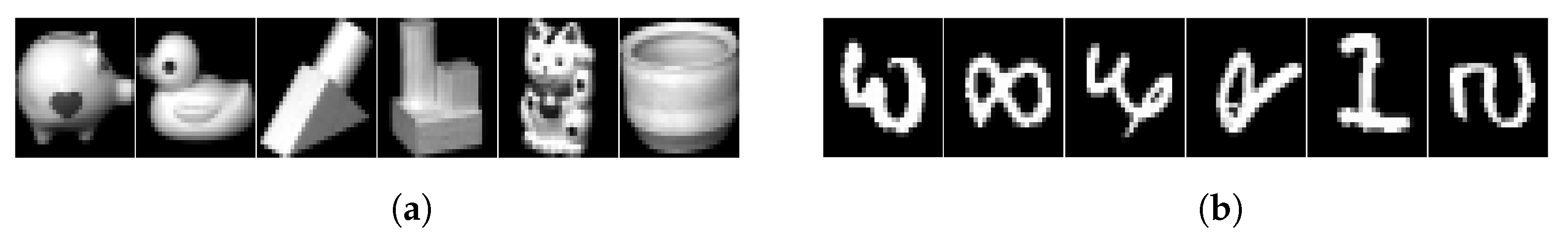
The six real datasets used include two small datasets, two medium datasets, and two large datasets. The two small datasets are COIL20 [40], a 32 × 32 grayscale image of 20 different classes of objects, totaling 1440 samples, and MNISTSC2000, a variant of the MNIST dataset [41], where we select a total of 2000 samples from different classes and downscale them to 500 by principal component analysis. The two medium datasets are PenDights [42], a UCI dataset [43] containing 10 features and 10 classes with 10,992 samples, and MNIST [41], which is a 28 × 28 grayscale image of handwritten digits from 0–9, with 60,000 training samples and 10,000 test samples. The two large datasets are UCI datasets [43]. One is CovType [42], which contains 54 features and 7 classes of 581,012 samples. The other is PokerHand [44], which contains 10 features and 10 classes of 1,000,000 samples. The details of all datasets are summarized in Table 2. Figure 2 shows some sample datasets.

Table 2. Details of the datasets used in the experiments.

Dataset	Sample	Dimensions	Classes
COIL20	1440	1024	20
MNISTSC2000	2000	500	10
PenDights	10,992	16	10
MNIST	70,000	784	10
CovType	581,012	54	7
PokerHand	1,000,000	10	10

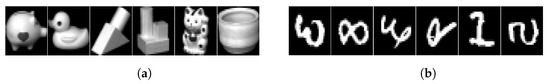
Figure 2. Sample images of some datasets used in the experiment. (a) COIL20; (b) MNIST.

4.2. Comparison Methods and Evaluation Metrics

To extensively evaluate the performance of the PKTLS${}^2$C model, we compare PKTLS${}^2$C with 13 state-of-the-art LS${}^2$C methods, including K-means [2], SEC [20], Nystr$\ddot{\mathrm{o}}$m [22], LSC-R [23], LSC-K [23], SSSC [1], SLRR [1], SLSR [1], PLrSC [34], RPCM${}_{l_1+F^2}$[17], RPCM${}_{l_1}$[17], RPCM${}_{\ast }$ [17], and RPCM${}_{F^2}$ [17]. The specifics of these methods were described in detail in the introduction section. To guarantee the fairness of the comparison experiments, we strictly follow the parameter settings in the original texts to optimize these methods in order to achieve their optimal results.

We choose two commonly used metrics, the clustering accuracy (ACC) and the normalized mutual information (NMI), to evaluate the clustering performance. For ACC and NMI, larger values indicate better clustering performance. Refer to [39] for the detailed definitions of ACC and NMI.

4.3. Parameter Settings and Analysis

In PKTLS${}^2$C, several parameter settings are involved, including kernel parameters, learning depth encoder parameters, sampling numbers, and balancing parameters. They are explained in detail as follows.

4.3.1. The Setting of Kernel Parameters

In order to better handle the nonlinear structure of the data, we set up a total of twelve basis kernel functions, including (1) seven Gaussian kernel functions with the same formula $K(x,y)=exp\left(\frac{{-\parallel x-y\parallel }_F^2}{{\sigma }^{2}d}\right)$. All have the same setting of $\sigma$, with the maximum distance between x and y in the dataset, but with different $d\in \{0.01,0.05,0.1,1,10,50,$$100\}$; (2) four polynomial kernel functions with the same formula $K(x,y)={\left(a+x^{T}y\right)}^b$, but different settings of $a\in \{0,1\}$ and $b\in \{2,4\}$; and (3) one linear kernel function $K(x,y)=x^{T}y$.

4.3.2. The Settings of Hidden Units and Layers

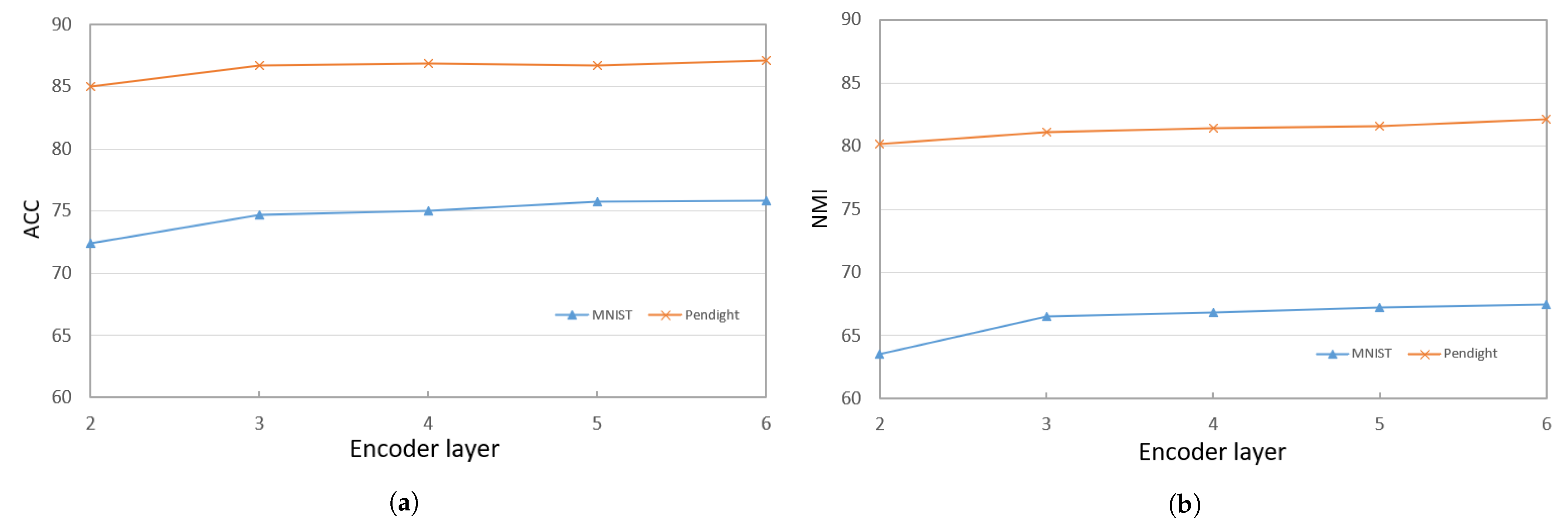
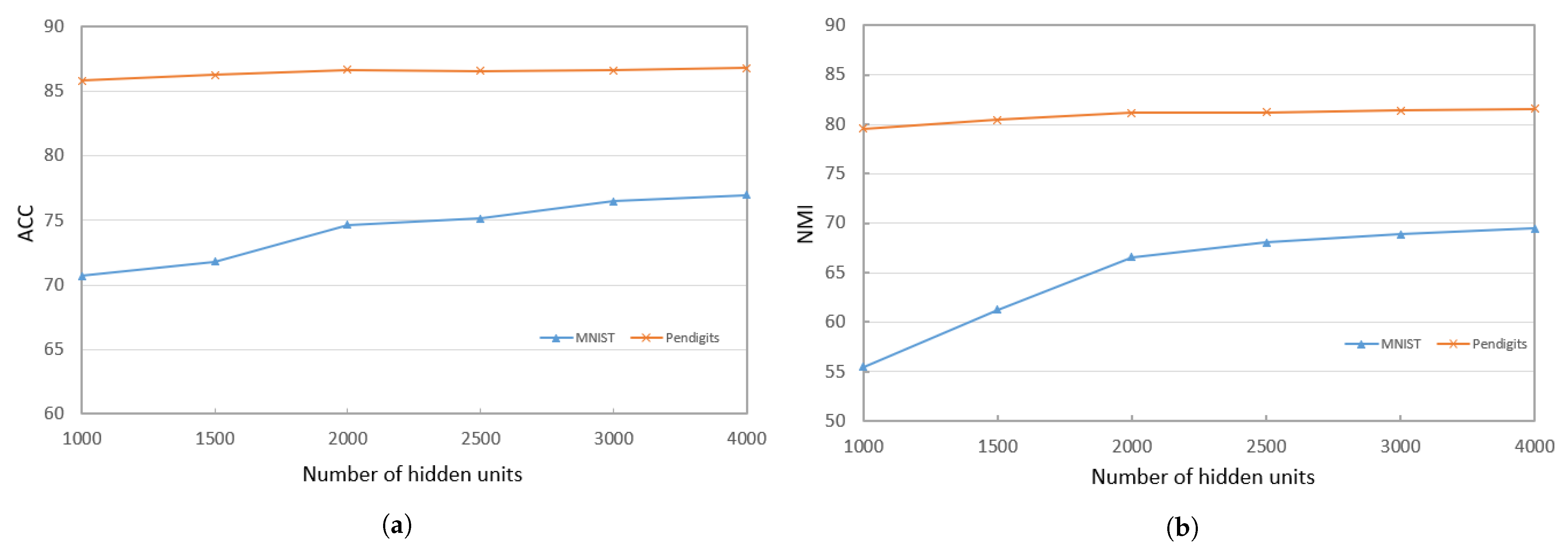
When training the deep encoder, we find that the performance of PKTLS${}^2$C is greatly related to the number of hidden units and the number of structural layers. Figure 3a,b show the ACCs and NMIs, respectively, with a fixed number of hidden units (2000) but varying the number of structural layers. Figure 4a,b show results with a fixed number of structural layers (3), but different numbers of hidden units, conducted on the PenDigits and MNIST datasets. This experiment achieved similar effects to other datasets, but due to space limitations, they are not presented in this paper.

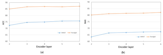
Figure 3. ACCs and NMIs of PKTLS${}^2$C with different numbers of structural layers and a fixed number of hidden units (2000) on the PenDights and MNIST datasets. (a) ACCs; (b) NMIs.

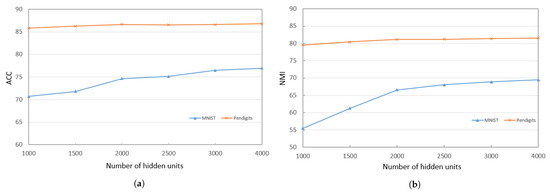
Figure 4. ACCs and NMIs of PKTLS${}^2$C with different numbers of hidden units and a fixed number of structural layers (3) on the PenDights and MNIST datasets. (a) ACCs; (b) NMIs.

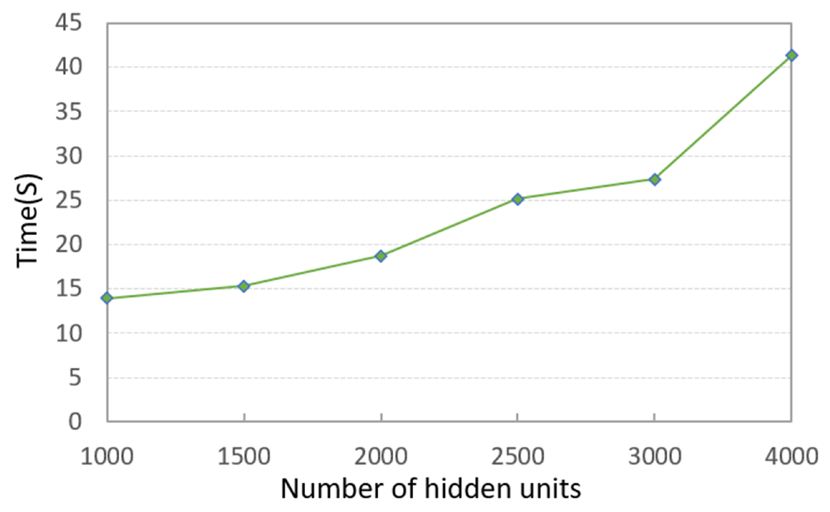
It can be seen that the PKTLS${}^2$C model achieves ideal ACCs and NMIs when the number of structural layers is ≥3 and the number of hidden units is ≥2000. As the number of hidden units increases, both ACCs and NMIs become larger, but this leads to longer execution times. Figure 5 shows the execution time in relation to the number of hidden units. In order to better balance the clustering performance and the execution time, we set the number of structural layers to 3 and the number of hidden units to 2000 in the following experiments:

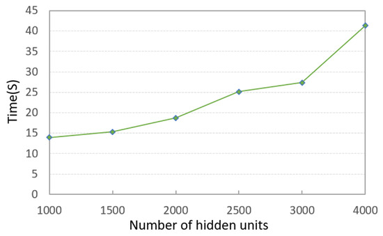
Figure 5. Execution times along with the number of hidden units and a fixed number of structural layers (3) on the MNIST dataset (in seconds).

4.3.3. Setting of Balance Parameters

The PKTLS${}^2$C model contains four equilibrium parameters: ${\lambda }_1$, ${\lambda }_2$, ${\lambda }_3$, and $\gamma$. Among them, ${\lambda }_1$, ${\lambda }_2$, and ${\lambda }_3$ are the parameters to equilibrate $\mathit{C}$, $\mathcal{P}$, and $\mathcal{E}$, respectively, and $\gamma$ is the parameter used to equilibrate ${\parallel \mathit{C}-f(\mathit{X},\omega )\parallel }_F^2$. To find the optimal parameters, we first simply set $\gamma$ to 1 [34], and then use the grid search method for the optimal ${\lambda }_1$, ${\lambda }_2$, ${\lambda }_3$, and set them to $\{{10}^{-4},{10}^{-3},{10}^{-2},{10}^{-1},1,10,20,30,50,100,1000\}$. Using PenDights as an example, the parameters’ sensitivity of the PKTLS${}^2$C model on this dataset is shown in Figure 6. It can be found that the PKTLS${}^2$C model is applicable to a wide range of ${\lambda }_1,{\lambda }_2,{\lambda }_3$ values.

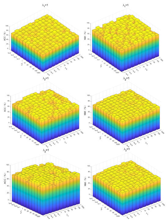
Figure 6. Parameter sensitivity of the PKTLS${}^2$C model on the PenDights dataset.

4.3.4. Effects of the Number of Samples

To evaluate the impacts of different sizes of sample datasets on the final clustering results, we run PKTLS${}^2$C on the PenDights dataset with different sample numbers; the results are shown in Figure 7. It can be seen that the PKTLS${}^2$C model has stable ACCs and NMIs that are not sensitive to the number of samples. So we can use small datasets to train the deep encoder and greatly shorten the training time. This experiment has also achieved similar effects on other datasets, but due to space constraints, it will not be presented here. This experiment has also achieved similar effects on other datasets, but due to space limitations, they are not presented in this paper.

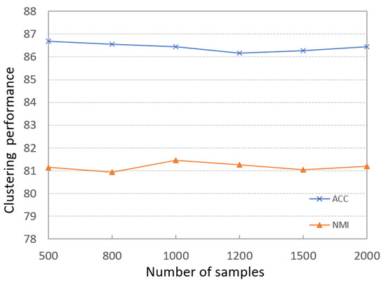
Figure 7. Effects of different scale sample data on clustering results on the PenDights dataset.

4.4. Comparison with Other Models

In this subsection, we compare the clustering performance of the PKTLS${}^2$C model with other models on the six datasets, where results for small datasets, medium datasets, and large datasets are shown in Table 3, Table 4 and Table 5, respectively. In addition, we add seven traditional subspace clustering methods on small-scale datasets (i.e., K-means [2], SSC [9], LRR [10], LKGr [45], JMKSC [46], LLMKL [47], and LRMKSC [39]) for comparison. Since these traditional methods are not applicable to medium and large datasets, we only use them on small datasets. We present the average and standard deviations of ACCs and NMIs in ten runs, where the optimal values of different algorithms are presented in bold font.

Table 3. Clustering results and execution times (in seconds) for small datasets.

Dataset		COIL20			MNISTSC2000
Number of Samples		n = 500			n = 500
Evaluation Indicators		ACC	NMI	Time	ACC	NMI	Time
	K-means	60.63 ± 1.2	75.78 ± 0.39	0.21	56.69 ± 0.1	55.79 ± 0.18	0.58
	SSC	45.64 ± 2.35	57.32 ± 0.98	6.18	79.3 ± 0.48	81.04 ± 0.36	14.28
	LRR	64.58 ± 3.24	76.95 ± 1.78	215.94	75.92 ± 2.53	76.30 ± 1.24	41.49
Conventional	LKGr	61.8 ± 3.13	76.6 ± 2.31	118.68	15.7 ± 2.03	5.6 ± 1.39	150.79
methods	JMKSC	62.1 ± 3.54	69.3 ± 1.53	40.88	76.5 ± 2.23	70.06 ± 1.53	60.39
	LLMKL	63.6 ± 1.02	80.6 ± 0.41	216.32	38.4 ± 0.96	23.6 ± 1.32	230.42
	LRMKSC	53.28 ± 3.25	62.27 ± 0.36	381.54	14.5 ± 1.53	1.4 ± 0.05	555.08
	LSC-K	70.35 ± 4.38	80.69 ± 2.1	0.62	80.64 ± 0.35	75.99 ± 0.63	0.83
	SSSC	32.72 ± 4.56	58.85 ± 3.3	11.71	—	—	—
	PLrSC	74.15 ± 4.13	85.62 ± 2.70	1.02	80.11 ± 4.58	76.36 ± 2.85	0.86
LS${}^2$C methods	RPCM${}_{\ast }$	82.7 ± 1.8	89.36 ± 1.3	7.03	95.45 ± 0.38	89.95 ± 0.73	4.26
	RPCM${}_F^2$	84.79 ± 2.14	90.8 ± 1.36	0.76	95.55 ± 0.33	90.26 ± 0.6	1.02
	ours	86.06 ± 1.0	91.17 ± 0.78	0.55	95.69 ± 0.24	90.17 ± 0.26	0.52

—indicates NAN or INF.

Table 4. Clustering results and execution times (in seconds) for medium datasets.

Dataset		PenDigits			MNIST
Number of Samples		n = 500			n = 500
Evaluation Indicators		ACC	NMI	Time	ACC	NMI	Time
	K-means	68.51 ± 0.13	68.79 ± 0.02	1.78	54.51 ± 1.85	49.23 ± 1.03	41.23
	SEC	75.3 ± 4.20	70.3 ± 2.43	11.8	57.43 ± 2.58	52.86 ± 1.26	14.68
	Nystr$\ddot{\mathrm{o}}$m	66.7 ± 6.93	65.4 ± 2.70	35.9	52.7 ± 1.46	47.4 ± 0.38	60.15
	LSC-R	77.7 ± 3.18	74.9 ± 2.61	5.6	59.74 ± 1.89	57.06 ± 1.36	6.45
	LSC-K	79.9 ± 2.73	76.4 ± 0.58	7.9	65.74 ± 2.59	62.06 ± 1.76	10.86
	SSSC	76.20 ± 0	68.88 ± 0	4.03	54.9 ± 1.89	49.9 ± 1.15	35.01
	SLRR	74.59 ± 0.12	67.18 ± 0.00	3.36	50.0 ± 3.87	49.1 ± 2.27	38.76
Methods	SLSR	68.83 ± 0.1	62.94 ± 0.05	3.2	54.1 ± 1.56	48.1 ± 0.87	31.23
	PLrSC	77.47 ± 3.04	76.43 ± 2.39	2.59	65.18 ± 4.37	61.55 ± 1.62	12.77
	RPCM${}_{l_1+F^2}$	85.71 ± 1.4	80.5 ± 1.6	6.15	66.36 ± 3.0	58.93 ± 2.48	21.44
	RPCM${}_{l_1}$	80.99 ± 2.5	72.36 ± 2.1	7.27	—	—	—
	RPCM${}_{\ast }$	85.5 ± 0.8	80.75 ± 1.5	2.91	64.17 ± 3.21	58.86 ± 2.71	22.09
	RPCM${}_F^2$	85.7 ± 1.63	79.94 ± 1.7	2.23	66.43 ± 3.38	61.3 ± 1.7	19.95
	ours	86.68 ± 0.19	81.14 ± 0.53	1.07	74.68 ± 3.1	66.57 ± 0.62	18.73

—indicates NAN or INF.

Table 5. Clustering results and execution times (in seconds) for large datasets.

Dataset		CovType			PokerHand
Number of Samples		n = 1000			n = 500
Evaluation Indicators		ACC	NMI	Time	ACC	NMI	Time
	K-means	20.8 ± 0.00	3.7 ± 0.00	156.6	10.47 ± 0.05	0.04 ± 0.00	169.3
	SEC	21.1 ± 0.01	3.6 ± 0.00	84.9	10.5 ± 0.06	0.1 ± 0.01	130.2
	Nystr$\ddot{\mathrm{o}}$m	24.0 ± 0.59	3.8 ± 0.03	70.6	10.91 ± 0.15	0.08 ± 0.03	184.4
	LSC-R	22.0 ± 0.47	3.8 ± 0.06	154.5	12.6 ± 0.17	0.1 ± 0.04	205.7
	LSC-K	22.0 ± 0.52	3.6 ± 0.10	955.4	12.32 ± 0.51	0.1 ± 0.02	1736.8
	SSSC	27.8 ± 0.16	4.56 ± 0.04	173.5	15.34 ± 0.42	0.1 ± 0.01	212.15
	SLRR	27.24 ± 0.00	6.35 ± 0.02	120.11	15.40 ± 0.41	0.07 ± 0.10	217.7
Methods	SLSR	26.53 ± 0.00	4.2 ± 0.00	168.8	12.79 ± 0.44	0.06 ± 0.01	194.2
	PLrSC	24.87 ± 1.03	5.31 ± 0.36	53.89	12.71 ± 0.32	0.01 ± 0.03	152.05
	RPCM${}_{l_1+F^2}$	26.2 ± 0.28	2.32 ± 0.16	354.62	11.65 ± 0.28	0.1 ± 0.00	962.98
	RPCM${}_{l_1}$	23.76 ± 1.72	2.41 ± 0.15	309.15	13.08 ± 0.14	0.1 ± 0.00	751.55
	RPCM${}_{\ast }$	26.01 ± 0.09	1.35 ± 0.63	514.26	11.35 ± 0.08	0.1 ± 0.00	928.04
	RPCM${}_F^2$	23.66 ± 0.53	3.75 ± 0.11	360.97	11.92 ± 0.92	0.1 ± 0.00	926.97
	ours	28.37 ± 1.3	3.2 ± 0.1	73.44	16.46 ± 0.2	0.5 ± 0.03	167.48

In this paper, the size of the sample dataset is 500, except for the CovType dataset. This is because the comparison method needs 1000 samples on CovType to obtain the result, as in [1]. To obtain a fair comparison, we set the sample number to 1000 for CovType.

Overall. From Table 3, Table 4 and Table 5, we find that the PKTLS${}^2$C method achieves the best results compared to the other methods in the six datasets. In particular, the average ACC and NMI values of PKTLS${}^2$C improve by up to 8.25% and 4.97% compared to the suboptimal values on the MNIST dataset. In addition, the running time of the PKTLS${}^2$C method is shorter than all other methods on the four medium and large datasets. It is also shorter than all other methods except for K-means on the two small datasets,

Small datasets. From Table 3, we find that PKTLS${}^2$C achieves significant improvement compared with the traditional methods. For example, compared with the best one achieved by the traditional methods, PKTLS${}^2$C increases the average ACC and NMI by 19.48% and 19.22%, respectively, on the COIL20 dataset, and 16.39% and 9.15%, respectively, on the MNISTSC2000 dataset. This is because PKTLS${}^2$C uses a secondary denoising method, which can effectively highlight the structural feature of the dataset and minimize the impact of noise on the clustering task. This is also demonstrated in the following robustness and visualization experiments. Except for K-means, the other traditional subspace clustering methods are based on spectral clustering, which leads to high computational complexity. However, PKTLS${}^2$C learns the feature information of the original dataset from a trained deep encoder with a small sample dataset, greatly reducing the computational complexity. For example, the running times of LRR on the COIL20 and MNISTSC2000 datasets are about 400 times longer than PKTLS${}^2$C’s. For the same reason, all LS${}^2$C methods require considerably less time than traditional methods on both datasets.

Medium datasets. From Table 4, we find that PKTLS${}^2$C also achieves the best ACCs and NMIs compared to other state-of-the-art LS${}^2$C-based methods. For example, on the PenDigits dataset, PKTLS${}^2$C increases the average ACC and NMI values by 0.9% and 0.39% compared with the other best ones, even reaching 8.25% and 4.97% on the MNIST dataset. Among the compared methods, RPCM${}_{l_1+F^2}$, RPCM${}_{l_1}$, RPCM${}_{\ast }$, RPCM${}_{F^2}$, and PKTLS${}^2$C all use deep encoders to predict the feature information of the original large dataset and they perform better than other LS${}^2$C-based methods. This indicates the effectiveness of using deep self-encoders for the prediction of large dataset feature information. Moreover, during the process of selecting a small sample dataset to train the deep encoder, we use MKL to deal with the nonlinear structure of datasets, and we use to tensor to capture the higher-order correlations among datasets. So, PKTLS${}^2$C allows the trained deep encoder to obtain the data feature information as comprehensively as possible, guaranteeing the reliability of its clustering performance.

Large datasets. Table 5 shows the experiments on large datasets, even reaching 1,000,000 units in the PokerHand dataset. Different from the four datasets in Table 3 and Table 4, these two datasets are more challenging. From Table 5, we find that all methods perform very poor on NMI for both datasets, which is caused by the highly imbalanced clustering. Therefore, we only compare ACC. PKTLS${}^2$C, on average, improves ACC by 0.57% compared to the suboptimal one on the CovType dataset, and it reaches 1.06% on the PokerHand dataset. The running time of PKTLS${}^2$C is also the shortest among all the compared methods and takes substantially less time to perform the clustering task. This indicates that PKTLS${}^2$C can be applied to LS${}^2$C tasks with high clustering efficiency.

4.5. Robustness Analysis

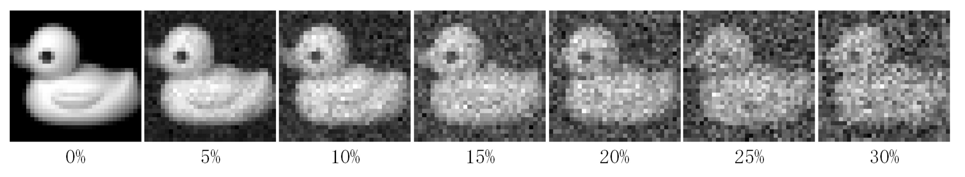
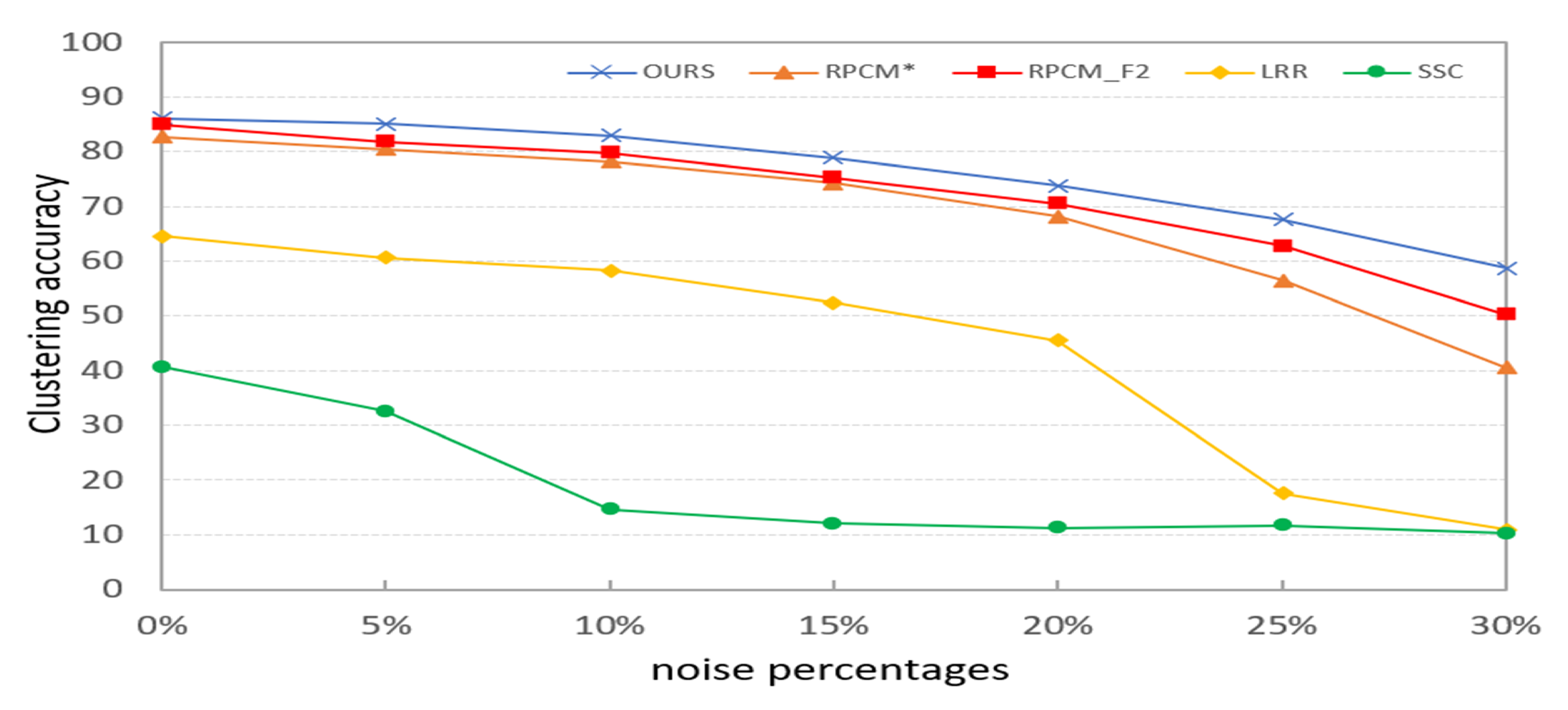
In this section, we verify the robustness of PKTLS${}^2$C. We select the robust LS${}^2$C methods (RPCM${}_{\ast }$ and RPCM${}_{F^2}$) and conventional methods (SSC and LRR) as the compared methods. As shown in Figure 8, we add a certain percentage (5%, 10%, 15%, 20%, 25%, and 30%) of random noises to the COIL20 dataset. Then, we perform clustering tasks on them separately and use ACC to evaluate the clustering performance of the methods with different proportions of noises. According to Figure 9, we find that the clustering performance of all methods decreases as the proportion of noise increases. But PKTLS${}^2$C achieves the best clustering results in all cases. It shows that our proposed quadratic denoising method in PKTLS${}^2$C can efficiently enhance the clustering robustness. This experiment also achieved similar effects on other datasets, but due to space limitations, they are not presented in this paper.

Figure 8. Visualization of the COIL20 data with different noise ratios.

Figure 9. Effects of different proportions of noises on the clustering performance on the COIL20 dataset.

4.6. Visualization

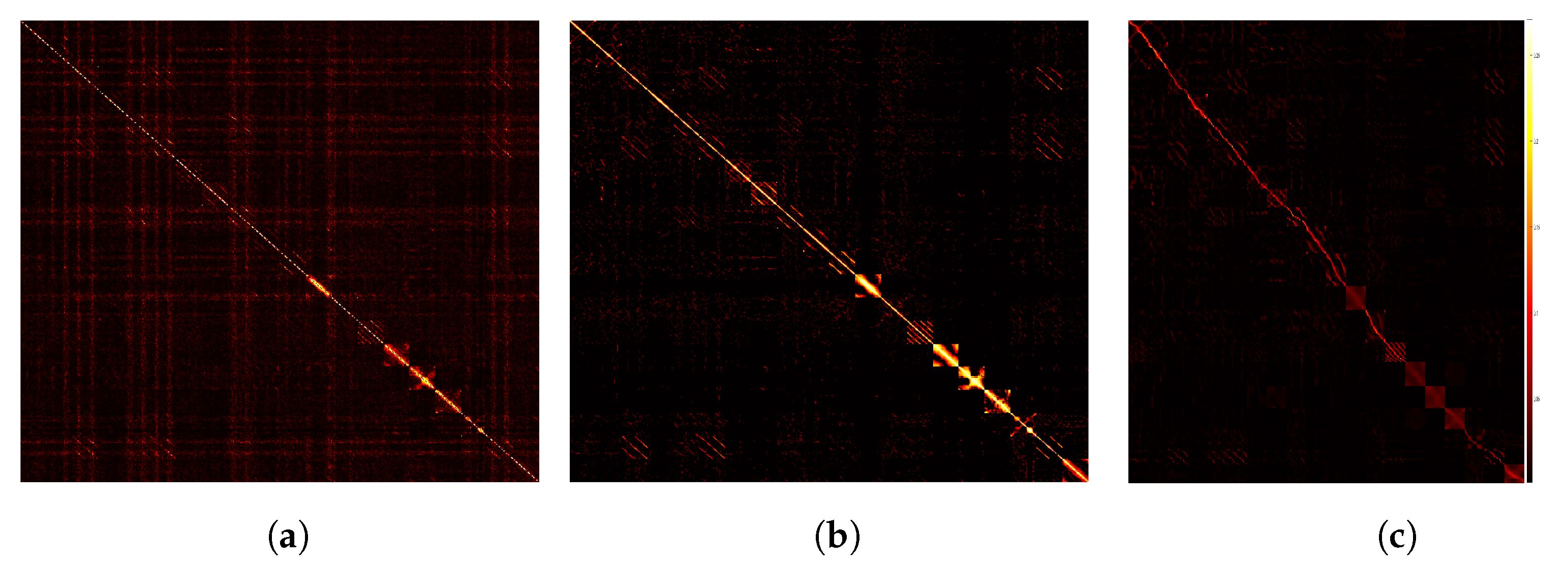
In this section, we use the small-scale dataset, COIL20, to show the prediction results of the feature information by the trained deep encoder. We compare the affinity matrix generated by PKTLS${}^2$C with SSC and LRR, as shown in Figure 10. From Figure 10, we find that PKTLS${}^2$C can efficiently process the structure of the original dataset. The inter-cluster structure in the low-rank representation matrix of the original data generated by PKTLS${}^2$C is more clearly visible than the other two, which provides the basis for accurate identification in subsequent clustering tasks. This also ensures that PKTLS${}^2$C is applicable to large datasets. In addition, the low-rank representation matrix data generated by PKTLS${}^2$C is purer than those generated by SSC and LRR, further demonstrating the robustness of PKTLS${}^2$C.

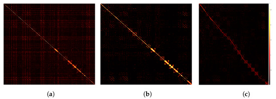
Figure 10. Comparison of visualizations on the COIL20 dataset. (a) SSC; (b) LRR; (c) PKTLS${}^2$C.

4.7. Convergence Analysis

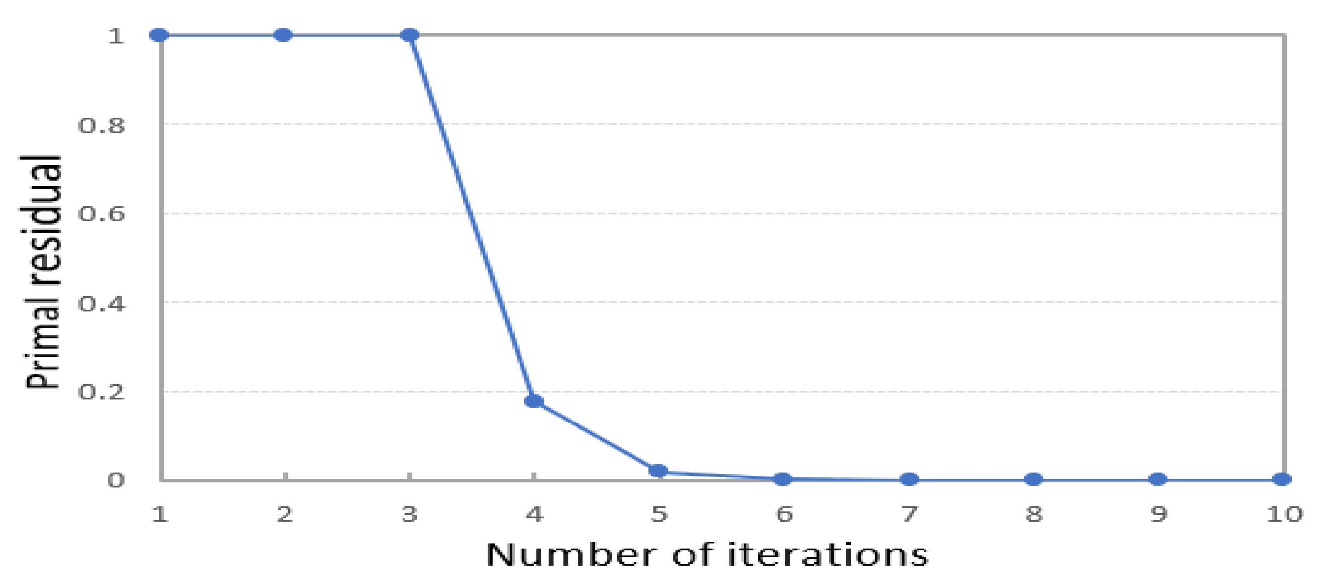
According to Equation (2), solving the SE matrix $\mathit{C}$ of the sample dataset is related to the training of the deep encoder. In PKTLS${}^2$C, to guarantee fast convergence in training the deep encoder, we simply constrain the solved residual values of the sample dataset’s SE matrix $\mathit{C}$. Therefore, we set the following convergence condition:

$$\begin{array}{c}\hfill max\left({∥{\mathit{C}}^{t+1}-{\mathit{C}}^t∥}_{\infty }\right)\le 1\mathrm{e}-4.\end{array}$$

(33)

When the residual is less than 1e − 4, the model meets the convergence condition and the iteration stops. The setting of this parameter belongs to the setting of experience value. Figure 11 shows the residuals of the MNIST dataset in each iteration of the solving process of PKTLS${}^2$C. We find that PKTLS${}^2$C converges and smooths out within a relatively small number of iterations. This experiment also achieved similar effects on other datasets, but due to space limitations, they are not presented in this paper.

Figure 11. Convergence curve variation of the PKTLS${}^2$C method on the MNIST dataset.

It is normal that residuals do not decrease during the first three iterations. The reason is that we use the gradient descent method in the optimization process, which may lead to escaping local optimal solutions in the iterative search space to find a better solution, which may result in instances where the residual does not decrease.

5. Conclusions

In this paper, we propose an efficient LS${}^2$C method—PKTLS${}^2$C. PKTLS${}^2$ uses a small sample dataset to train the deep encoder, and then applies it to the original large dataset, which can quickly obtain a projection sparse-coded representation of the large dataset. Extensive experiments on large datasets show that PKTLS${}^2$C achieves higher accuracy and a higher convergence rate compared to existing LS${}^2$C methods. In addition, we propose purity kernel tensor learning and secondary denoising methods, which help PKTLS${}^2$C capture more valid information and further improve the robustness of the model. Moreover, we executed extensive experiments to analyze the parameters of the learned deep encoder, verifying its feasibility in performing subspace clustering tasks. Future work will focus on optimizing the processing of the sample dataset to obtain more useful information for training the deep encoder.

References

- Peng, X.; Tang, H.; Zhang, L.; Yi, Z.; Xiao, S. A unified framework for representation-based subspace clustering of out-of-sample and large-scale data. IEEE Trans. Neural Netw. Learn. Syst. 2015, 27, 2499–2512. [Google Scholar] [CrossRef] [PubMed]
- MacQueen, J. Classification and analysis of multivariate observations. In Proceedings of the 5th Berkeley Symposium on Mathematical Statistics and Probability, San Diego, CA, USA, 21 June–18 July 1967; pp. 281–297. [Google Scholar]
- Li, Q.; Xie, Z.; Wang, L. Robust Subspace Clustering with Block Diagonal Representation for Noisy Image Datasets. Electronics 2023, 12, 1249. [Google Scholar] [CrossRef]
- Fan, L.; Lu, G.; Liu, T.; Wang, Y. Block Diagonal Least Squares Regression for Subspace Clustering. Electronics 2022, 11, 2375. [Google Scholar] [CrossRef]
- Yin, L.; Lv, L.; Wang, D.; Qu, Y.; Chen, H.; Deng, W. Spectral Clustering Approach with K-Nearest Neighbor and Weighted Mahalanobis Distance for Data Mining. Electronics 2023, 12, 3284. [Google Scholar] [CrossRef]
- Liu, M.; Liu, C.; Fu, X.; Wang, J.; Li, J.; Qi, Q.; Liao, J. Deep Clustering by Graph Attention Contrastive Learning. Electronics 2023, 12, 2489. [Google Scholar] [CrossRef]
- Ng, A.; Jordan, M.; Weiss, Y. On spectral clustering: Analysis and an algorithm. Adv. Neural Inf. Process. Syst. 2001, 14, 849–856. [Google Scholar]
- Hou, C.; Nie, F.; Yi, D.; Tao, D. Discriminative embedded clustering: A framework for grouping high-dimensional data. IEEE Trans. Neural Netw. Learn. Syst. 2014, 26, 1287–1299. [Google Scholar] [PubMed]
- Elhamifar, E.; Vidal, R. Sparse subspace clustering: Algorithm, theory, and applications. IEEE Trans. Pattern Anal. Mach. Intell. 2013, 35, 2765–2781. [Google Scholar] [CrossRef]
- Liu, G.; Lin, Z.; Yan, S.; Sun, J.; Yu, Y.; Ma, Y. Robust recovery of subspace structures by low-rank representation. IEEE Trans. Pattern Anal. Mach. Intell. 2012, 35, 171–184. [Google Scholar] [CrossRef]
- Lu, C.Y.; Min, H.; Zhao, Z.Q.; Zhu, L.; Huang, D.S.; Yan, S. Robust and efficient subspace segmentation via least squares regression. In Proceedings of the European Conference on Computer Vision, Florence, Italy, 7–13 October 2012; Springer: Berlin/Heidelberg, Germany, 2012; pp. 347–360. [Google Scholar]
- Fan, J. Large-Scale Subspace Clustering via k-Factorization. In Proceedings of the 27th ACM SIGKDD Conference on Knowledge Discovery & Data Mining, Singapore, 14–18 August 2021; pp. 342–352. [Google Scholar]
- Pourkamali-Anaraki, F. Large-scale sparse subspace clustering using landmarks. In Proceedings of the 2019 IEEE 29th International Workshop on Machine Learning for Signal Processing (MLSP), Pittsburgh, PA, USA, 13–16 October 2019; IEEE: New York, NY, USA, 2019; pp. 1–6. [Google Scholar]
- Wang, S.; Tu, B.; Xu, C.; Zhang, Z. Exact subspace clustering in linear time. In Proceedings of the AAAI Conference on Artificial Intelligence, Quebec, QB, Canada, 27–31 July 2014; Volume 28. [Google Scholar]
- Zhang, X.; Tan, Z.; Sun, H.; Wang, Z.; Qin, M. Orthogonal Low-rank Projection Learning for Robust Image Feature Extraction. IEEE Trans. Multimed. 2021, 24, 3882–3895. [Google Scholar] [CrossRef]
- Wang, H.; Kawahara, Y.; Weng, C.; Yuan, J. Representative selection with structured sparsity. Pattern Recognit. 2017, 63, 268–278. [Google Scholar] [CrossRef]
- Li, J.; Liu, H.; Tao, Z.; Zhao, H.; Fu, Y. Learnable subspace clustering. IEEE Trans. Neural Netw. Learn. Syst. 2020, 33, 1119–1133. [Google Scholar] [CrossRef] [PubMed]
- Li, J.; Tao, Z.; Wu, Y.; Zhong, B.; Fu, Y. Large-scale subspace clustering by independent distributed and parallel coding. IEEE Trans. Cybern. 2021, 52, 9090–9100. [Google Scholar] [CrossRef] [PubMed]
- Li, B.; Zhang, Y.; Lin, Z.; Lu, H. Subspace clustering by mixture of gaussian regression. In Proceedings of the IEEE Conference on Computer Vision and Pattern Recognition, Boston, MA, USA, 7–11 June 2015; pp. 2094–2102. [Google Scholar]
- Nie, F.; Zeng, Z.; Tsang, I.W.; Xu, D.; Zhang, C. Spectral embedded clustering: A framework for in-sample and out-of-sample spectral clustering. IEEE Trans. Neural Netw. 2011, 22, 1796–1808. [Google Scholar] [PubMed]
- Chen, W.Y.; Song, Y.; Bai, H.; Lin, C.J.; Chang, E.Y. Parallel spectral clustering in distributed systems. IEEE Trans. Pattern Anal. Mach. Intell. 2010, 33, 568–586. [Google Scholar] [CrossRef] [PubMed]
- Fowlkes, C.; Belongie, S.; Chung, F.; Malik, J. Spectral grouping using the Nystrom method. IEEE Trans. Pattern Anal. Mach. Intell. 2004, 26, 214–225. [Google Scholar] [CrossRef]
- Cai, D.; Chen, X. Large scale spectral clustering via landmark-based sparse representation. IEEE Trans. Cybern. 2014, 45, 1669–1680. [Google Scholar]
- Yan, D.; Huang, L.; Jordan, M.I. Fast approximate spectral clustering. In Proceedings of the 15th ACM SIGKDD International Conference on Knowledge Discovery and Data Mining, Virtual Event, 6–10 July 2009; pp. 907–916. [Google Scholar]
- Wright, J.; Yang, A.Y.; Ganesh, A.; Sastry, S.S.; Ma, Y. Robust face recognition via sparse representation. IEEE Trans. Pattern Anal. Mach. Intell. 2008, 31, 210–227. [Google Scholar] [CrossRef]
- You, C.; Li, C.G.; Robinson, D.P.; Vidal, R. Oracle based active set algorithm for scalable elastic net subspace clustering. In Proceedings of the IEEE Conference on Computer Vision and Pattern Recognition, Las Vegas, NV, USA, 27–30 June 2016; pp. 3928–3937. [Google Scholar]
- You, C.; Li, C.; Robinson, D.P.; Vidal, R. Scalable exemplar-based subspace clustering on class-imbalanced data. In Proceedings of the European Conference on Computer Vision (ECCV), Munich, Germany, 8–14 September 2018; pp. 67–83. [Google Scholar]
- Kang, Z.; Lin, Z.; Zhu, X.; Xu, W. Structured graph learning for scalable subspace clustering: From single view to multiview. IEEE Trans. Cybern. 2021, 52, 8976–8986. [Google Scholar] [CrossRef]
- Bourlard, H.; Kamp, Y. Auto-association by multilayer perceptrons and singular value decomposition. Biol. Cybern. 1988, 59, 291–294. [Google Scholar] [CrossRef]
- Ranzato, M.; Poultney, C.; Chopra, S.; Cun, Y. Efficient learning of sparse representations with an energy-based model. Adv. Neural Inf. Process. Syst. 2006, 19, 819006. [Google Scholar]
- Vincent, P.; Larochelle, H.; Bengio, Y.; Manzagol, P.A. Extracting and composing robust features with denoising autoencoders. In Proceedings of the 25th International Conference on Machine Learning, Helsinki, Finland, 5–9 July 2008; pp. 1096–1103. [Google Scholar]
- Sprechmann, P.; Bronstein, A.M.; Sapiro, G. Learning efficient sparse and low rank models. IEEE Trans. Pattern Anal. Mach. Intell. 2015, 37, 1821–1833. [Google Scholar] [CrossRef] [PubMed]
- Gregor, K.; LeCun, Y. Learning fast approximations of sparse coding. In Proceedings of the 27th International Conference on International Conference on Machine Learning, Haifa, Israel, 21–24 June 2010; pp. 399–406. [Google Scholar]
- Li, J.; Liu, H. Projective low-rank subspace clustering via learning deep encoder. In Proceedings of the IJCAI, Melbourne, Australia, 19–25 August 2017. [Google Scholar]
- Ripley, B.D. Pattern Recognition and Neural Networks; Cambridge University Press: Cambridge, UK, 2007. [Google Scholar]
- Haykin, S. Neural Networks and Learning Machines, 3/E; Pearson Education: Chennai, India, 2009. [Google Scholar]
- Liu, X.; Zhou, S.; Wang, Y.; Li, M.; Dou, Y.; Zhu, E.; Yin, J. Optimal neighborhood kernel clustering with multiple kernels. In Proceedings of the AAAI Conference on Artificial Intelligence, San Francisco, CA, USA, 4–9 February 2017; Volume 31. [Google Scholar]
- Gönen, M.; Alpaydın, E. Multiple kernel learning algorithms. J. Mach. Learn. Res. 2011, 12, 2211–2268. [Google Scholar]
- Zhang, X.; Xue, X.; Sun, H.; Liu, Z.; Guo, L.; Guo, X. Robust multiple kernel subspace clustering with block diagonal representation and low-rank consensus kernel. Knowl. Based Syst. 2021, 227, 107243. [Google Scholar] [CrossRef]
- Nene, S.A.; Nayar, S.K.; Murase, H. Columbia Object Image Library (Coil-20); Columbia University: New York, NY, USA, 1996. [Google Scholar]
- LeCun, Y.; Bottou, L.; Bengio, Y.; Haffner, P. Gradient-based learning applied to document recognition. Proc. IEEE 1998, 86, 2278–2324. [Google Scholar] [CrossRef]
- Alimoglu, F.; Alpaydin, E. Combining multiple representations and classifiers for pen-based handwritten digit recognition. In Proceedings of the Fourth International Conference on Document Analysis and Recognition, Ulm, Germany, 18–20 August 1997; IEEE: New York, NY, USA, 1997; Volume 2, pp. 637–640. [Google Scholar]
- Dua, D.; Graff, C. UCI Machine Learning Repository. Available online: http://archive.ics.uci.edu/ml (accessed on 1 December 2023).
- Blackard, J.A.; Dean, D.J. Comparative accuracies of artificial neural networks and discriminant analysis in predicting forest cover types from cartographic variables. Comput. Electron. Agric. 1999, 24, 131–151. [Google Scholar] [CrossRef]
- Kang, Z.; Wen, L.; Chen, W.; Xu, Z. Low-rank kernel learning for graph-based clustering. Knowl. Based Syst. 2019, 163, 510–517. [Google Scholar] [CrossRef]
- Yang, C.; Ren, Z.; Sun, Q.; Wu, M.; Yin, M.; Sun, Y. Joint correntropy metric weighting and block diagonal regularizer for robust multiple kernel subspace clustering. Inf. Sci. 2019, 500, 48–66. [Google Scholar] [CrossRef]
- Ren, Z.; Li, H.; Yang, C.; Sun, Q. Multiple kernel subspace clustering with local structural graph and low-rank consensus kernel learning. Knowl. Based Syst. 2020, 188, 105040. [Google Scholar] [CrossRef]
Disclaimer/Publisher’s Note: The statements, opinions and data contained in all publications are solely those of the individual author(s) and contributor(s) and not of MDPI and/or the editor(s). MDPI and/or the editor(s) disclaim responsibility for any injury to people or property resulting from any ideas, methods, instructions or products referred to in the content. |
© 2023 by the authors. Licensee MDPI, Basel, Switzerland. This article is an open access article distributed under the terms and conditions of the Creative Commons Attribution (CC BY) license (https://creativecommons.org/licenses/by/4.0/).