Optimization of an Operation Strategy for Variable Speed Pumped Storage Power System Flexibility

Abstract

With the increase in the grid-connected scale of new energy, the ability to flexibility regulate a power system is greatly challenged. Since a variable speed pumped storage (VSPS) unit has a wider power regulation range and higher operation efficiency than conventional pumped storage (CPS), this study focuses on improving system flexibility with the VSPS unit. First, the probabilistic characteristics of forced outages affecting the flexibility of power units are studied. Considering the uncertainty of the net load prediction error, a probabilistic density method is proposed to quantify the flexibility of the power system. Second, in order to improve the flexibility of the system and take into account the comprehensive benefits of the VSPS unit, an optimization model for the VSPS unit to improve the flexibility of the grid was established based on bacterial colony chemotaxis that takes into consideration the operational constraints of the VSPS unit. Finally, to verify the effectiveness of the proposed optimization strategy using simulation, the proposed optimization model is used to compare the advantages of the VSPS unit’s ability to regulate system flexibility with a conventional pumped storage unit.

1. Introduction

Increasing the installation capacity of new energy resources is an important measure for both coping with global climate change and realizing the goals of peak carbon emissions and carbon neutrality [1,2]; however, the output of new energy resources are characterized by strong random fluctuations caused by changes in the season and climate. These features not only result in increasing demand uncertainty of the grid net load, but also may cause reverse peak load regulation phenomena. As the scale of new energy resources integrated into the power grid increases, the capacity of the power grid to use reserve capacity for peak load regulation and load change climbing tracking is challenged even more [3,4]. Power system flexibility refers to the capacity of rapidly responding to the uncertainty in the changes in balancing the power supply and load demands while considering operational and economic constraints [5]. Since the power grid reserve capacity will be reduced by replacing traditional synchronous generators with new energy resources and the output uncertainty of the new energy resources will affect the power grid’s flexibility demand of peak load regulation and load change climbing tracking, the power grid has to use different measures, such as wind and photovoltaic curtailment or load shedding, when resource flexibility is insufficient. In this case, it is important to determine how to improve the regulation flexibility of the new energy grid-connected power system.

As a practical energy storage technology for power systems, pumped storage has the characteristics of rapid start and stop, stable operation and minimal influence from natural factors [6]; thus, it has been widely used to improve the operation characteristics of new energy grid-connected power systems [7,8,9]. The literature [10] establishes a coordinated operation model of wind power and pumped storage from the perspective of reducing wind abandonment in the power grid and reflects the important role of pumped storage in balancing the supply–demand relationship between the source and load side of the system by comparing the changes in the total amount of wind abandonment of the system before and after the participation of pumped storage in the operation. The literature [11] constructs a multi-timescale optimal scheduling model based on the complementary operating characteristics of the combined wind-optical-thermal power-pumped storage-battery system and verifies that the scheduling strategy is effective in improving the regulation capability of the power system. In the literature [12], a combined wind-light-water-fire-pumped storage system is constructed, and the uncertainty of wind and light output is processed using the pumped storage plant in the system, and the optimal multi-region dynamic and economic dispatch model is solved by chaotic fast-converging evolutionary planning. It is worth pointing out that the above optimization strategy for pumped storage to improve the system’s peaking and load to balance supply and demand uses the total amount of wind and light abandonment to reflect the system’s peaking flexibility, and there is a lack of discussion on how to quantify the flexibility of the system’s peaking and ramping capacity by taking into account the impact of uncertainty factors. In addition, there is insufficient consideration of the operating characteristics of the unit, such as the difference in the unit power regulation capability under pumping and generating conditions, and the unit operating efficiency does not consider the impact of the unit operating efficiency decreasing with the output power decline. Moreover, VSPS are not considered as the regulation object.

Compared with conventional pumped storage (CPS) units, variable speed pumped storage (VSPS) units can improve the operation efficiency of the turbine by adjusting the rotational speed under pumped and power generation conditions and expand the power regulation range of the unit. Therefore, its more flexible power regulation ability allows it to improve system stability and provides economic benefits during operation by improving dynamic characteristics, and its ability to absorb new energy power fluctuations has been studied [13,14,15]. Consequently, this paper focuses on the optimization operation strategy of VSPS to improve the flexibility of power grid regulation. The method of quantifying the lack of flexibility using probability density is studied on the basis of considering the uncertainty of system flexibility. Second, with reference to research on electromechanical transient modeling and operation characteristics of VSPS in the literature [16,17,18], an optimization model of VSPS considering the constraints of VSPS’s operational constraints to improve the operation strategy of the system’s regulation flexibility was constructed. Finally, the effectiveness of the optimization method proposed is verified using simulation.

2. Methods for Quantifying Inflexibility Taking Uncertainty into Account

2.1. Probabilistic Analysis of the Impact of Forced Outages of Conventional Thermal Units on System Flexibility

Currently, thermal power units are an essential resource for flexible regulation of the grid. On one hand, the decrease in the unit start-up rate caused by the integration of new energy grids will affect the peaking and ramping capacity, which reflects the flexibility supply capacity of the system. On the other hand, the uncertain forced outage of the grid-connected units will also have a dynamic impact on the peaking and climbing capacity of the system. Therefore, how to quantify the impact of forced outages on the peaking and climbing capacity of units is an important basis for rational optimization and flexible regulation of other resources in the system. All of the on-loaded units in the system are ordered according to the unit operating cost from smallest to largest following the principle that the next unit is loaded until the previous sorted unit reaches the maximum technological output. Therefore, the literature [19,20] uses two-state probability to propose Equations (1) and (2) to quantify the probability distribution expressions for the impact of forced outages on the upward peaking capacity $G_{\mathrm{G}i}^{\mathrm{up}}$, downward peaking capacity $G_{\mathrm{G}i}^{\mathrm{dp}}$, upward climbing capacity $R_{\mathrm{G}i}^{\mathrm{ur}}$ and downward climbing capacity $R_{\mathrm{G}i}^{\mathrm{dr}}$ of the units.

$$\{\begin{array}{l}{g}_{\mathrm{G}i}^{\mathrm{up}}=\{\begin{array}{lll}{P}_{\mathrm{G}i}^{\max }& ,& 1-p_{\mathrm{G}i}^{\mathrm{stop}}\\ 0& ,& p_{\mathrm{G}i}^{\mathrm{stop}}\end{array}\\ g_{\mathrm{G}i}^{\mathrm{dp}}=\{\begin{array}{lll}{P}_{\mathrm{G}i}^{\min }& ,& 1-p_{\mathrm{G}i}^{\mathrm{stop}}\\ 0& ,& p_{\mathrm{G}i}^{\mathrm{stop}}\end{array}\\ G_{\mathrm{G}i}^{\mathrm{up}}=g_{\mathrm{G}1}^{\mathrm{up}}\times g_{\mathrm{G}2}^{\mathrm{up}}\times \cdot \cdot \cdot \times g_{\mathrm{G}i}^{\mathrm{up}}\\ G_{\mathrm{G}i}^{\mathrm{dp}}=g_{\mathrm{G}1}^{\mathrm{dp}}\times g_{\mathrm{G}2}^{\mathrm{dp}}\times \cdot \cdot \cdot \times g_{\mathrm{G}i}^{\mathrm{dp}}\end{array}$$

(1)

Here, $P_{\mathrm{G}i}^{\max }$ and $P_{\mathrm{G}i}^{\min }$ are the maximum and minimum technical output of thermal power unit I, respectively; $p_{\mathrm{G}i}^{\mathrm{stop}}$ is the forced outage rate of unit I; $g_{\mathrm{G}i}^{\mathrm{up}}$ and $g_{\mathrm{G}i}^{\mathrm{dp}}$ are the probability distributions of the up and down peaking capacity of unit i, respectively; and $G_{\mathrm{G}i}^{\mathrm{up}}$ and $G_{\mathrm{G}i}^{\mathrm{dp}}$ are the probability distributions of the up and down peaking capacity of the system after loading i unit, respectively, which are determined by the convolution of the probability distributions of the upward and downward peaking capacity of the loaded units.

$$\{\begin{array}{l}{r}_{Gi}^{\mathrm{ur}}=\{\begin{array}{ll}\{\begin{array}{lll}{r}_{\mathrm{G}i}^u\Delta t& ,& 1-p_{\mathrm{G}i}^{\mathrm{stop}}\\ 0& ,& p_{\mathrm{G}i}^{\mathrm{stop}}\end{array}& (R_{\mathrm{G}i}^{\min }\le P_{\mathrm{G}i}^t\le R_{\mathrm{G}i}^{\max })\\ 0& (P_{\mathrm{G}i}^t=P_{\mathrm{G}i}^{\max })\end{array}\\ r_{Gi}^{\mathrm{dr}}=\{\begin{array}{ll}\{\begin{array}{lll}{r}_{\mathrm{G}i}^d\Delta t& ,& 1-p_{\mathrm{G}i}^{\mathrm{stop}}\\ 0& ,& p_{\mathrm{G}i}^{\mathrm{stop}}\end{array}& (R_{\mathrm{G}i}^{\min }\le P_{\mathrm{G}i}^t\le R_{\mathrm{G}i}^{\max })\\ 0& (P_{\mathrm{G}i}^t=P_{\mathrm{G}i}^{\min })\end{array}\\ R_{\mathrm{G}i}^{\mathrm{ur}}=r_{\mathrm{G}1}^{\mathrm{ur}}\times r_{\mathrm{G}2}^{\mathrm{ur}}\times \cdot \cdot \cdot \times r_{\mathrm{G}i}^{\mathrm{ur}}\\ R_{\mathrm{G}i}^{\mathrm{dr}}=r_{\mathrm{G}1}^{\mathrm{dr}}\times r_{\mathrm{G}2}^{\mathrm{dr}}\times \cdot \cdot \cdot \times r_{\mathrm{G}i}^{\mathrm{dr}}\end{array}$$

(2)

Here, $r_{\mathrm{G}i}^{\mathrm{u}}$ and $r_{\mathrm{G}i}^{\mathrm{d}}$ are the ramp rates for upward and downward power regulation of unit I, respectively; $\Delta t$ denotes the unit power regulation time; $r_{\mathrm{G}i}^{\mathrm{ur}}$ and $r_{\mathrm{G}i}^{\mathrm{dr}}$ are the probability distributions of the upward and downward ramping capacities of unit output power during $\Delta t$, respectively; $R_{\mathrm{G}i}^{\max }$ and $R_{\mathrm{G}i}^{\min }$ denote the technical output power of unit i before $P_{\mathrm{G}i}^{\max }$ and $P_{\mathrm{G}i}^{\min }$ during $\Delta t$, respectively, where $R_{\mathrm{G}i}^{\max }$ = $P_{\mathrm{G}i}^{\max }$ − $r_{\mathrm{G}i}^{\mathrm{u}}\Delta t$, $R_{\mathrm{G}i}^{\min }$ = $P_{\mathrm{G}i}^{\min }$ + $r_{\mathrm{G}i}^{\mathrm{d}}\Delta t$; and $R_{\mathrm{G}i}^{\mathrm{ur}}$ and $R_{\mathrm{G}i}^{\mathrm{dr}}$ are the probability distributions of the upward and downward climbing capacity during $\Delta t$ after the startup of unit i. They are determined by the convolutional calculation of the probability distribution of the upward and downward climbing capacity at time t for each start-up unit.

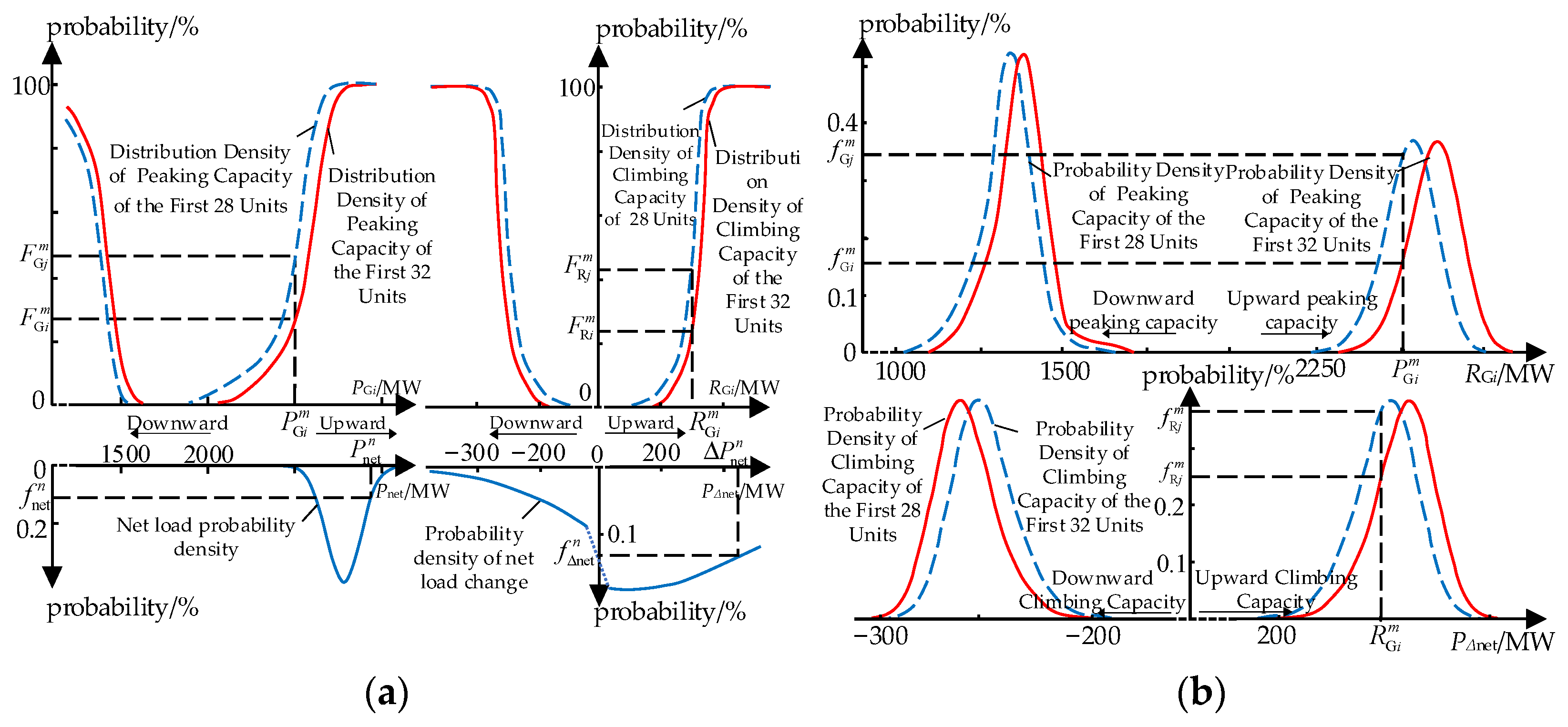
Considering the characteristics of the forced outage two-state distribution leading to discrete values for the computed results of $g_{\mathrm{G}i}^{\mathrm{up}}$, $g_{\mathrm{G}i}^{\mathrm{dp}}$, $r_{\mathrm{G}i}^{\mathrm{ur}}$ and $r_{\mathrm{G}i}^{\mathrm{dr}}$ after the convolution solution of $G_{\mathrm{G}i}^{\mathrm{up}}$, $G_{\mathrm{G}i}^{\mathrm{dp}}$, $R_{\mathrm{G}i}^{\mathrm{ur}}$ and $R_{\mathrm{G}i}^{\mathrm{dr}}$ using the semi-invariant method, the convolution results are further expanded based on the Gram-Charlier series, which can change the discrete probability distributions of the system’s peaking and climbing capacities into continuous probability distribution curves [21]. The probability distribution curves of the peaking and climbing capacities at the time of startup of the first 28 and the first 32 units reported in Table A1 of Appendix A can be calculated in accordance with the method above, and the results are presented in Figure 1a. Due to the existence of maximum and minimum technical output limitations of the units, the upward and downward effective peaking range of the system will increase and decrease, respectively, with the increase in the units. When the upward and downward peaking demand is the same, the probability of the system’s upward and downward effective peaking capacity shortfalls will decrease and increase, respectively, as the loaded units increase. In addition, as the maximum upward and downward effective climbing regulation range increases, the probability of the effective climbing capacity shortfall decreases with the same demand for upward and downward climbing capacities.

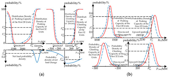
Figure 1. Probability distribution and density distribution of the insufficient capacity of both peak-regulating and ramp-climbing. (a) Density distribution, (b) Probability distribution.

Derivation of the probability distribution curves yields the probability density curves $f_{\mathrm{up}}(P_{\mathrm{G}i}^m)$ and $f_{\mathrm{dp}}(P_{\mathrm{G}i}^m)$ for the upward and downward peaking capacity corresponding to $P_{\mathrm{G}i}^m$(m = 1, 2,…, ∞) and the probability density curves $f_{\mathrm{ur}}(R_{\mathrm{G}i}^{\mathrm{ur},m}\Delta t)$ and $f_{\mathrm{dr}}(R_{\mathrm{G}i}^{\mathrm{dr},m}\Delta t)$ for the upward and downward climbing capacity $R_{\mathrm{G}i}^{\mathrm{ur},m}\Delta t$ after loading first i units as shown in Figure 1b. As noted in the figure, the capacity range enclosed by the probability density curves of upward and downward effective peaking capacity is shifted to the left and right sides of the horizontal coordinate axis, respectively, as the number of units loaded increases, and the capacity range enclosed by the probability density curves of the upward and downward effective creeping capacity shortage is shifted to the left and right sides of the horizontal coordinate axis, respectively, with the increase in the number of units loaded.

2.2. Quantification of System Flexibility Based on Probability Density

The system’s flexibility can be calculated by the flexibility supply minus the demand. A positive result indicates that the flexibility of the system is sufficient; otherwise, the system flexibility is insufficient. Random shutdown of the unit and net load forecast error will make the peak and climbing capacities of the system and net load forecast in a certain range of distribution randomly. From the perspective of uncertainty, the difference between the net load demand of the system and the upward effective peaking capacity as the amount of load shedding of the system due to insufficient upward peaking capacity can be obtained by using the dual integration shown in Equation (3).

$$\{\begin{array}{l}{P}_{\mathrm{net}}^n~N(P_{\mathrm{load}}-P_{\mathrm{RE}},{\delta }_{RE}^2+{\delta }_{\mathrm{load}}^2)\\ P_{\mathrm{up}}^{mn}=\{\begin{array}{c}{P}_{\mathrm{net}}^n-P_{\mathrm{G}i}^m,\\ 0,\end{array}\begin{array}{c}{P}_{\mathrm{net}}^n>P_{\mathrm{G}i}^m\\ P_{\mathrm{net}}^n\le P_{\mathrm{G}i}^m\end{array}\\ P_{\mathrm{up}}={\displaystyle {\int }_{-\infty }^{\infty }({\displaystyle {\int }_0^{P_{\mathrm{net}}^n}{P}_{\mathrm{up}}^{mn}{f}_{\mathrm{G}i}^{m}d}}{P}_{\mathrm{G}i})f_{\mathrm{net}}^{n}d{P}_{net}\end{array}$$

(3)

Here, $P_{\mathrm{RE}}$ and $P_{\mathrm{load}}$ are the new energy unit output and load demand prediction values, respectively. The prediction error can be obtained according to the value of the normal distribution. If not specified, in this study, the wind power serves as the new energy research object. ${\delta }_{\mathrm{RE}}$ and ${\delta }_{\mathrm{load}}$ are the predicted standard deviations of the new energy unit output and load demand, respectively. $P_{\mathrm{net}}^n$ is the corrected value of the net system load taking into account the forecast error, namely, the total system flexibility requirements. $P_{\mathrm{G}i}^m$ is the effective peaking capacity after loading first i units. $P_{\mathrm{up}}^{mn}$ is the amount of load shedding on the system due to insufficient upward peaking capacity. $f_{\mathrm{G}i}^m$ is the probability density value corresponding to $P_{\mathrm{G}i}^m$. $f_{\mathrm{net}}^n$ is the probability density value corresponding to net load $P_{\mathrm{net}}^n$.

Similarly, the difference between the system’s upward climbing capacity and the net load climbing demand as the amount of load cut by the system due to insufficient upward climbing capacity can be obtained utilizing the dual integration shown in Equation (4).

$$\{\begin{array}{l}{P}_{\mathrm{ur}}^{mn}=\{\begin{array}{c}\Delta P_{\mathrm{net}}^n-R_{\mathrm{Gi}}^m\Delta t,\\ 0,\end{array}\begin{array}{c}\Delta P_{\mathrm{net}}^n>R_{\mathrm{Gi}}^m\Delta t\\ \Delta P_{\mathrm{net}}^n\le R_{\mathrm{Gi}}^m\Delta t\end{array}\\ P_{\mathrm{ur}}={\displaystyle {\int }_0^{\infty }({\displaystyle {\int }_0^{\Delta P_{\mathrm{net}}^n}{P}_{\mathrm{ur}}^{mn}{f}_{\mathrm{R}i}^{m}d}}{R}_{\mathrm{G}i})f_{\Delta \mathrm{net}}^{n}d\Delta P_{net}\end{array}$$

(4)

Here, $\Delta P_{\mathrm{net}}^n$ is the predicted climb of the system’s net load, $R_{\mathrm{Gi}}^m\Delta t$ is the upward effective climbing capacity after loading the first i units, $f_{\mathrm{R}i}^m$ is the probability density corresponding to $R_{\mathrm{Gi}}^m\Delta t$, and $f_{\Delta \mathrm{net}}^n$ is the probability density corresponding to the net load creep demand $\Delta P_{\mathrm{net}}^n$.

Similarly, the calculation method for wind abandonment due to insufficient downward effective peaking capacity of the system $P_{\mathrm{dp}}$ and wind abandonment due to insufficient downward effective climbing capacity $P_{\mathrm{dr}}$ can be obtained, and their values are both negative. The larger absolute values of $P_{\mathrm{up}}$ and $P_{\mathrm{ur}}$ reflect the lack of power according to insufficient of upward flexibility, and the larger absolute values of $P_{\mathrm{dp}}$ and $P_{\mathrm{dr}}$ reflect the lack of power according to insufficient downward flexibility. Therefore, the load cutting or wind abandonment caused by the lack of system flexibility is defined as follows:

$$P_{\mathrm{psf}}^t=\max (P_{\mathrm{up}}^t,P_{\mathrm{ur}}^t)+\min (P_{\mathrm{dp}}^t,P_{\mathrm{dr}}^t)$$

(5)

A positive result in Equation (5) indicates that the system has a load-shedding demand at time t due to insufficient upward regulation flexibility; otherwise, the system has a wind abandonment demand due to insufficient downward regulation flexibility.

3. Operational Optimization Model for Variable-Speed Pumped Storage Units to Enhance Grid Flexibility

3.1. Objective Function

The VSPS unit is able to synergize with thermal units to meet net load peaking and climbing capacity needs through orderly scheduling of pumping and generation operating conditions. As a flexible resource, it is worthwhile to study the issue of improving system flexibility by optimizing operating conditions while taking the operational benefits of flexibility regulation into account. Therefore, the objective function is established by considering the minimum loss of wind abandonment and load shedding caused by system inflexibility as well as the maximum operational benefit of flexibility regulation:

$$\max (\Delta C_{\mathrm{PSF}}+CI)$$

(6)

Here, $\Delta C_{\mathrm{psf}}$ is the total reduction of wind abandonment or load-shedding cost losses due to insufficient system flexibility after the VSPS unit is connected to the grid. CI is the operation income of the VSPS unit, for which $\Delta C_{\mathrm{psf}}$ is calculated as noted in Equation (7):

$$\{\begin{array}{l}{C}_{\mathrm{psf}}^t=\left|p_{\mathrm{LE}}\max (P_{\mathrm{up}}^t,P_{\mathrm{ur}}^t)+p_{\mathrm{LW}}\min (P_{\mathrm{dp}}^t,P_{\mathrm{dr}}^t)\right|T\\ \Delta C_{\mathrm{psf}}={\displaystyle \sum _{t=1}^N(C_{\mathrm{psf}}^{t0}-C_{\mathrm{psf}}^t)}\end{array}$$

(7)

where $P_{\mathrm{up}}^t$ and $P_{\mathrm{ur}}^t$ are the amount of load shedding at time t due to insufficient upward peaking and climbing capacity, respectively; $P_{\mathrm{dp}}^i$ and $P_{\mathrm{dr}}^i$ are wind abandonment due to the insufficient of downward peaking and climbing capacity, respectively; $p_{\mathrm{LW}}$ and $p_{\mathrm{LE}}$ are the penalty prices for load-shedding and wind abandonment per unit of capacity, respectively, which are used to convert load-shedding or wind abandonment into the corresponding penalty costs; T is the length of the regulation period; N is the number of regulation periods; and $C_{\mathrm{psf}}^{t0}$ and $C_{\mathrm{psf}}^t$ are the total costs of load-shedding and wind abandonment losses due to insufficient system flexibility before and after VSPS regulation in the period of t, respectively. The net load predictions $P_{\mathrm{net}}^t$ to calculate $C_{\mathrm{psf}}^{t0}$ satisfy a normal distribution N($P_{\mathrm{load}}^t$ − $P_{\mathrm{RE}}^t$, ${\delta }_{RE}^2$ + ${\delta }_{\mathrm{load}}^2$), and the net load predictions $P_{\mathrm{net}}^t$ to calculate $C_{\mathrm{psf}}^t$ use a normal distribution N($P_{\mathrm{load}}^i$ − $P_{\mathrm{RE}}^i$ + $P_{\mathrm{VSPS}}^t$, ${\delta }_{RE}^2$ + ${\delta }_{\mathrm{load}}^2$).

CI in Equation (6) denotes the maximum benefit that can be obtained within the operational limits of a VSPS unit participating in regulation. With reference to the two-part pricing method, the VSPS operating efficiency mainly takes into account the electricity tariff in the process of purchasing and selling electricity, the capacity tariff, the compensation tariff for peak shifting, and the cost loss caused by mechanical wear and tear in the switching of operating conditions. The maximum operational benefit calculations of the VSPS unit are reported as follows:

$$\{\begin{array}{l}\begin{array}{l}CI={\displaystyle \sum _{i=1}^N(C_{\mathrm{s}}^t+C_{\mathrm{g}}^t-C_{\mathrm{b}}^t)+}{C}_{\mathrm{c}}-C_{\mathrm{n}}\\ C_{\mathrm{s}}^t=\{\begin{array}{c}-p_{\mathrm{s}}^t{P}_{\mathrm{VSPS}}^{t}T,\\ 0,\end{array}\begin{array}{c}{P}_{\mathrm{VSPS}}^t<0\\ P_{\mathrm{VSPS}}^t\ge 0\end{array}\end{array}\hfill \\ C_{\mathrm{g}}^t=\{\begin{array}{c}{p}_{\mathrm{G}}^t{P}_{\mathrm{VSPS}}^{t}T,\\ 0,\end{array}\begin{array}{c}{P}_{\mathrm{VSPS}}^t\ge 0\\ P_{\mathrm{VSPS}}^t<0\end{array}\hfill \\ C_{\mathrm{b}}^t=\{\begin{array}{c}{p}_{\mathrm{b}}^t{P}_{\mathrm{VSPS}}^{t}T,\\ 0,\end{array}\begin{array}{c}{P}_{\mathrm{VSPS}}^t\ge 0\\ P_{\mathrm{VSPS}}^t<0\end{array}\hfill \\ C_{\mathrm{c}}=p_{\mathrm{c}}NT\max \left|P_{\mathrm{vsps}}^t\right|\hfill \\ C_{\mathrm{n}}={\displaystyle \sum _{t=1}^N{p}_{\mathrm{n}}(n_{\mathrm{on}}^t+n_{\mathrm{off}}^t)}\hfill \end{array}$$

(8)

where $C_{\mathrm{s}}^t$ and $C_{\mathrm{g}}^t$ are the income of the VSPS unit in the period of t determined by the selling tariff and the peaking compensation tariff, respectively; $C_{\mathrm{b}}^t$ is the cost determined by the power purchase tariff in time period t; $C_{\mathrm{c}}$ is the income determined by the capacity tariff; $C_{\mathrm{n}}$ is the cost incurred by starting and stopping the unit; $P_{\mathrm{VSPS}}^t$ is the regulation power of the VSPS unit in time period t, for which a positive value indicates that the VSPS unit is operating in pumping condition otherwise in generating condition; $p_{\mathrm{s}}^t$ and $p_{\mathrm{b}}^t$ are the unit cost of electricity sold and purchased in time period t, respectively; $p_{\mathrm{G}}^t$ is the carbon incentive compensation tariff due to the participation of the VSPS unit in flexibility regulation in time period t; $p_{\mathrm{c}}$ is the capacity tariff of the VSPS per unit of time; $p_{\mathrm{n}}$ is the loss of a single startup and shutdown of the unit; and $n_{\mathrm{on}}^t$ and $n_{\mathrm{off}}^t$ are symbolic variables for the presence of a startup and shutdown in time period t, respectively, with 1 indicating startup and 0 indicating shutdown.

3.2. Constraints

3.2.1. Unit Output Range Constraints

Compared with CPS units, VSPS units can output a wider range of power. Typically, the minimum output power of a VSPS unit under power generation conditions is 30–40% of the rated power, and the maximum output power is the rated power. The operating range of the units under pumping conditions is 70–100% of the rated power [22].

$$\left|P_{\mathrm{VSPS}}^{\min }\right|\le \left|P_{\mathrm{VSPS}}^t\right|\le \left|P_{\mathrm{VSPS}}^{\max }\right|$$

(9)

Here, $P_{\mathrm{VSPS}}^{\max }$ and $P_{\mathrm{VSPS}}^{\min }$ are the maximum and minimum output power allowed for the VSPS unit, respectively, and the values are related to the operating conditions of the units.

3.2.2. Reservoir Capacity Change Constraints

In order to prevent the VSPS from affecting the regulation capability of the next regulation cycle due to the large change in reservoir capacity after the N × T regulation cycle, the constraints on the change in the reservoir capacity during the regulation cycle are set in the optimization model. Then, the constraints on the change in reservoir capacity and water volume caused by the participation of the VSPS unit in flexibility regulation are transformed into the constraints on the upper and lower limits of the energy storage of the unit in order to facilitate optimization and solving:

$$\{\begin{array}{l}{E}_{\mathrm{VSPS}}^{\min }\le E_{\mathrm{VSPS}}^t\le E_{\mathrm{VSPS}}^{\max }\\ (1-\delta )E_{\mathrm{VSPS}}^0\le E_{\mathrm{VSPS}}^{N*T}\le (1+\delta )E_{\mathrm{VSPS}}^0\\ E_{\mathrm{VSPS}}^t=\{\begin{array}{c}{E}_{\mathrm{VSPS}}^{t-1}+f_{\mathsf{\eta }}(P_{\mathrm{VSPS}}^t)P_{\mathrm{VSPS}}^{t}T,\\ E_{\mathrm{VSPS}}^{t-1}+P_{\mathrm{VSPS}}^{t}T/f_{\mathsf{\eta }}(P_{\mathrm{VSPS}}^t),\end{array}\begin{array}{c}{P}_{\mathrm{VSPS}}^t\ge 0\\ P_{\mathrm{VSPS}}^t<0\end{array}\end{array}$$

(10)

where $E_{\mathrm{VSPS}}^t$ is the energy storage value of the VSPS unit at the end of time period t, and $E_{\mathrm{VSPS}}^0$ is the initial energy storage value for the current regulation cycle of variable speed pumping. In addition, $E_{\mathrm{VSPS}}^{\max }$ and $E_{\mathrm{VSPS}}^{\min }$ are the upper and lower limit values of the unit’s energy storage, respectively, and the greater the difference between the upper and lower limits, the more favorable it is for the unit to participate in flexibility regulation. $f_{\mathsf{\eta }}(P_{\mathrm{VSPS}0}^t)$ is the formula for calculating the energy conversion efficiency of the unit, which is related to the operating conditions and $P_{\mathrm{VSPS}0}^t$ [23]. $\delta$ is the maximum allowable percentage change in energy for the VSPS unit during the regulation cycle, and the greater $\delta$ is, the better the unit’s participation in regulating system flexibility.

3.2.3. Startup and Shutdown Constraints

In order to reduce the expenditure incurred by the unit due to frequent start-stop operations during the regulation cycle, constraints on the number of starts and stops of the unit are shown in Equation (11):

$$\{\begin{array}{l}\begin{array}{l}{n}_{\mathrm{on}}^t=\{\begin{array}{c}1,\mathrm{sgn}(\left|P_{\mathrm{VSPS}}^t\right|)-\mathrm{sgn}(\left|P_{\mathrm{VSPS}}^{t-1}\right|)=1\\ 0,\mathrm{sgn}(\left|P_{\mathrm{VSPS}}^t\right|)-\mathrm{sgn}(\left|P_{\mathrm{VSPS}}^{t-1}\right|)\ne 1\end{array}\\ n_{\mathrm{off}}^t=\{\begin{array}{c}1,\mathrm{sgn}(\left|P_{\mathrm{VSPS}}^t\right|)-\mathrm{sgn}(\left|P_{\mathrm{VSPS}}^{t-1}\right|)=-1\\ 0,\mathrm{sgn}(\left|P_{\mathrm{VSPS}}^t\right|)-\mathrm{sgn}(\left|P_{\mathrm{VSPS}}^{t-1}\right|)\ne -1\end{array}\end{array}\hfill \\ \begin{array}{l}{n}_{\mathrm{on}}={\displaystyle \sum _{t=1}^N{n}_{\mathrm{on}}^t}\le n_{\mathrm{on}}^{\max }\\ n_{\mathrm{off}}={\displaystyle \sum _{t=1}^N{n}_{\mathrm{off}}^t\le n_{\mathrm{off}}^{\max }}\end{array}\hfill \end{array}$$

(11)

where $n_{\mathrm{on}}$ and $n_{\mathrm{off}}$ are the total number of startups and shutdowns in the regulation cycle, respectively; and $n_{\mathrm{on}}^{\max }$ and $n_{\mathrm{off}}^{\max }$ are the maximum number of allowed startups and shutdowns, respectively. The larger the values are, the more the unit is able to participate in the system’s flexibility adjustment; therefore, the better the adjustment effect is. According to the equation, when the unit switches from shutdown to a generation operating status or pump operating condition at time t, the value of $n_{\mathrm{on}}^t$ is 1 and $n_{\mathrm{off}}^t$ is 0. When the unit switches from a generation operating status or pump operating condition to shutdown at time t, the value of $n_{\mathrm{on}}^t$ is 0 and $n_{\mathrm{off}}^t$ is 1. When there is a change from the pumping condition to the generating condition or a change from the generating condition to the pumping condition at time t, $n_{\mathrm{on}}^t$ is 1 and $n_{\mathrm{off}}^t$ is 1. $n_{\mathrm{on}}^t$ and $n_{\mathrm{off}}^t$ of each time are summed to obtain $n_{\mathrm{on}}$ and $n_{\mathrm{off}}$, respectively, and the values of $n_{\mathrm{on}}^{\max }$ and $n_{\mathrm{off}}^{\max }$ are limited to be no more than 3 and 4, respectively.

3.2.4. Constraints on the Number of Condition Transitions

In order to limit the number of switching times of the VSPS unit due to switching operating conditions to avoid the influence of frequent switching of operating conditions on its mechanical and electrical life cycle, the number of switching times of operating conditions is further established under the premise of setting up constraints on the number of startups and shutdowns:

$$\{\begin{array}{l}{n}_{\mathrm{cv}}^t=\{\begin{array}{c}1,\\ 0,\end{array}\begin{array}{c}{P}_{\mathrm{VSPS}}^{t-j}{P}_{\mathrm{VSPS}}^t<0\cap P_{\mathrm{VSPS}}^{t-j+1}{P}_{\mathrm{VSPS}}^k\ge 0\\ \mathrm{else}\end{array}\hfill \\ \begin{array}{l}t\ge j+1,k\in (t-j+1,i-1]\\ n_{\mathrm{cv}}={\displaystyle \sum _{t=1}^N{n}_{\mathrm{cv}}^t\le n_{\mathrm{cv}}^{\max }}\end{array}\hfill \end{array}$$

(12)

where $n_{\mathrm{cv}}^t$ is a sign variable for the presence or absence of a condition transition at time t. The presence of a condition transition is equal to one; otherwise, it is zero. $n_{\mathrm{cv}}$ and $n_{\mathrm{cv}}^{\max }$ are the total number of operating condition transitions and the maximum allowable number of VSPS units during the regulation cycle, respectively. The number of $n_{\mathrm{cv}}^{\max }$ is usually not greater than $n_{\mathrm{on}}^{\max }$ or $n_{\mathrm{off}}^{\max }$ because of shutdown caused by VSPS operation switching. The value of $n_{\mathrm{cv}}^{\max }$ needs to be determined according to the actual operational needs. However, the larger the value is, the better the effect of unit participating in the flexibility is. When the VSPS changes from the pumping condition to the generating condition or from the generating condition to the pumping condition at time t, $n_{\mathrm{cv}}^t$ is 1. Otherwise, it is 0. Summation of the values of $n_{\mathrm{cv}}^t$ in the time period of 1-N yields $n_{\mathrm{cv}}$, and the value of $n_{\mathrm{cv}}$ is limited to be no more than $n_{\mathrm{cv}}^{\max }$.

3.3. Optimized Model Solution

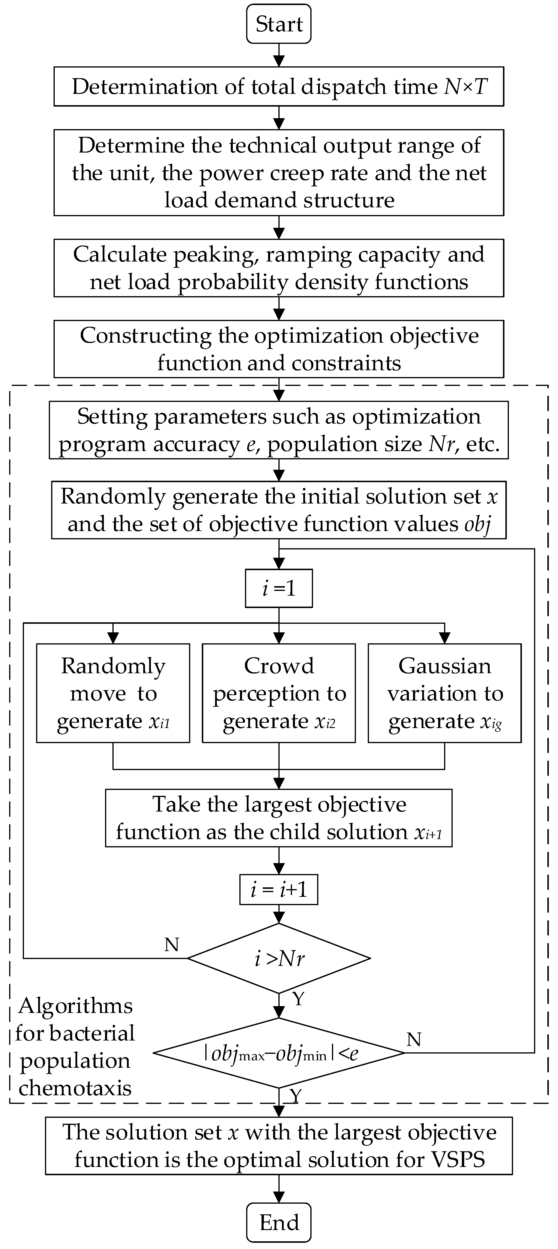
According to the established optimization model, the bacterial colony chemotaxis algorithm (BCC) is used for the optimal operation strategy of the VSPS unit to improve the system’s flexibility using the power scheduling instructions of the VSPS regulation cycle as the solution object. The specific method of calculation is shown in Figure 2.

Figure 2. Flowchart of using the bacterial colony chemotaxis algorithm to solve the optimization model.

As can be seen in the figure, the solution process begins by determining the length of the regulation period and the duration of each regulation period. The probability density function of the total system supply and demand power is analyzed based on the current parameters, such as the range of allowable output power of the grid-connected units, the power climbing rate, the probability of forced outages, and the net load forecasts for each time period taking into account the forecasting errors. Next, various parameters, such as the rated power of the VSPS unit, the upper and lower limits of the reservoir capacity, the maximum allowable number of operating condition transitions, and the maximum number of allowable startups and shutdowns, are determined, and the constraints shown in Equations (9)–(12) are established to optimize the power regulated by the VSPS unit. Meanwhile, in order to increase the solution speed of the optimization algorithm, based on Equation (13), the output power of the capacity of the VSPS unit participating in the regulation of system flexibility shortage in each time period is initialized according to the positive and negative polarity of the wind abandonment or load shedding caused by the system flexibility shortage in each time period obtained from the analysis. When the result of the system flexibility index is positive, the system abandons the wind due to a flexibility deficit. Then, the VSPS is stipulated to operate in the pumping condition. When the calculation result of the system flexibility index is negative, the system is not flexible enough to lead to load cutting. Then, the VSPS is stipulated to operate in the power generation condition. When the system’s flexibility is sufficient, the VSPS unit will not supply power.

$$\{\begin{array}{c}{P}_{\mathrm{VSPS}}^t<0,P_{\mathrm{PSF}}^t>0\\ P_{\mathrm{VSPS}}^t=0,P_{\mathrm{PSF}}^t=0\\ P_{\mathrm{VSPS}}^t>0,P_{\mathrm{PSF}}^t<0\end{array}$$

(13)

Based on the initialization preparations described above, the BCC algorithm is used to solve the power regulation strategy of the VSPS unit. The initial solution, which complies with Equations (9)–(13), is randomly generated, and new solutions x_i1, x_i2, and x_ig are generated for each particle of the solution set based on the individual random movement, the perceived population particle position, and the Gaussian variation, respectively. When the new solution does not satisfy the constraints, the objective function value is set to negative infinity, and the particle that maximizes the corresponding objective value is taken to be the child solution. Repeat the steps above until the difference between the best objective function values of the optimal solution and the worst solution within the population satisfies e or the number of iterations reaches the maximum limit. Then, the optimal solution in the last iteration is outputted as the optimal operation scheme for the VSPS unit. In the solution process, in order to speed up the algorithm solution and reduce the probability that the optimization-seeking particles fall into the local optimum, Equation (14) is used to adjust the perceptual range with the increase in the number of iterations, and the Gaussian noise shown in Equation (15) is introduced to make the degree of particle variation consistent with the normal distribution. Moreover, considering that the smaller the speed of the particles moving, the higher the accuracy of their search, Equation (16) is used to adjust the speed of the particles in order to improve the effectiveness of the search for particles in the process of searching for the optimal particle.

$$S=S_{\min }+(e^{\lambda \sigma }-1)/\lambda$$

(14)

$$x_g=x_i+N(0,\delta )$$

(15)

$$v^{n+1}=(v^n-v_{\min })e^{-\lambda n}+v_{\min }$$

(16)

Here, $S$ is the current generation particle perception range; $S_{\min }$ is the minimum value that limits the perception range; $\sigma$ is the degree of differentiation between particles in the population; $\lambda$ is the tuning parameter; $x_g$ is the particle position after the mutation; $x_i$ is the particle position before the mutation; $\delta$ is the Gaussian noise; n is the total number of iterations that have been performed in the optimization process; $v^n$ denotes the velocity of the particle in the nth iteration; and $v_{\min }$ is the minimum value of the particle velocity.

4. Example Analysis

4.1. Indicator Validity

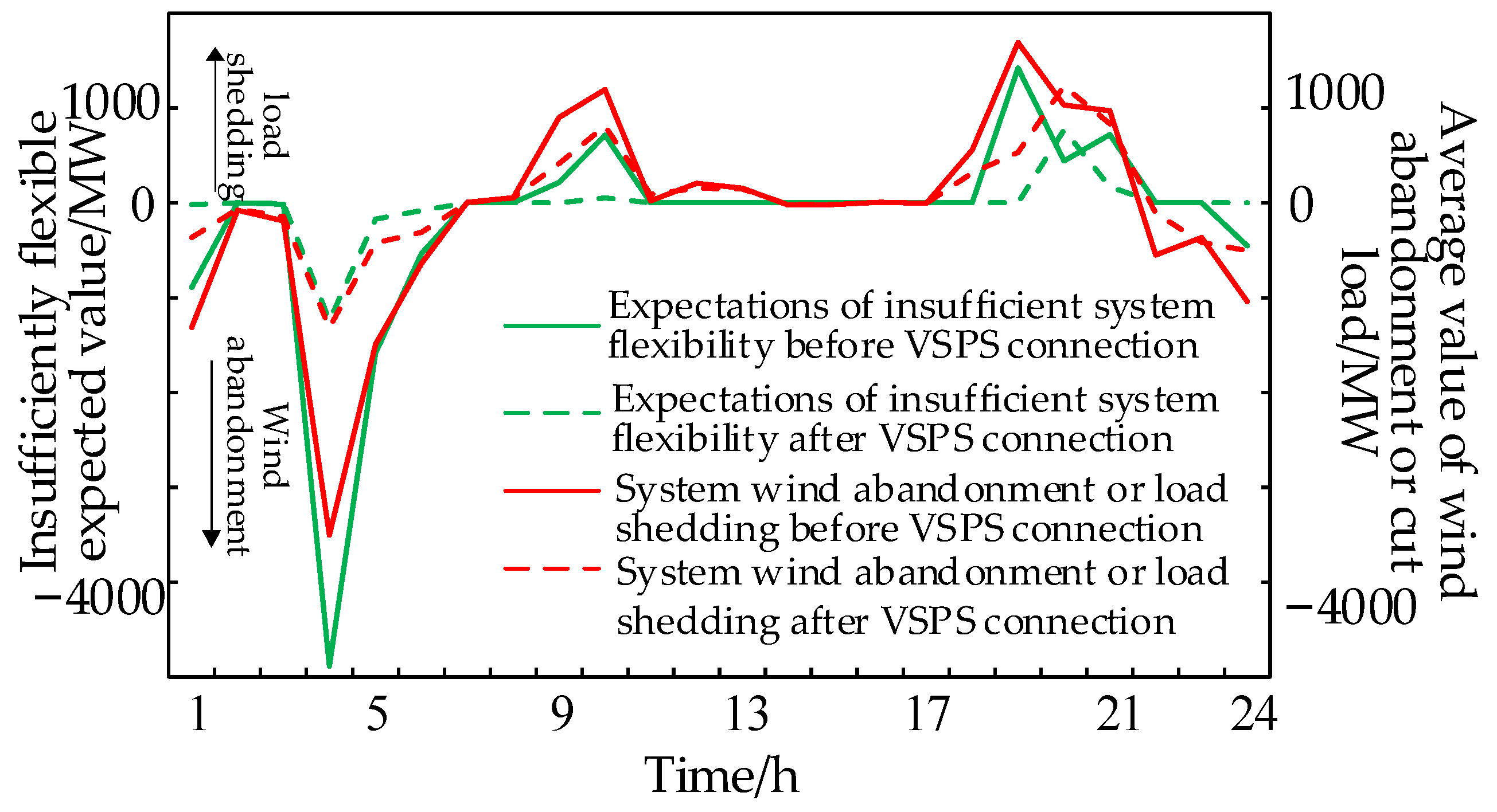
In order to verify the effectiveness of the proposed method for quantifying the system’s flexibility deficit considering the effects of uncertainties, such as forced unit shutdowns and net load forecast errors, the flexibility of the peaking and climbing capacity of the system containing conventional thermal power and new energy generation units over 24 h as shown in Table A2 of Appendix A is taken as the object of evaluation. Two methods of quantifying the amount of wind abandonment or load shedding caused by the flexibility deficit based on the expectation of flexibility deficit mentioned and this study’s quantification based on the probability density are used for the evaluation, respectively. Without considering the VSPS output range and capacity constraint limitations, the calculation results of this study’s inflexibility quantification method are used to set the VSPS output, so that the output of the VSPS unit in each time period is the same as the amount of wind abandonment or load shedding in the system due to the inflexibility. In other words, the unit works in the generation condition when upward flexibility is insufficient, and the unit works in the pumping condition when downward flexibility is insufficient. The results of using two types of flexibility quantification methods are shown in Figure 3.

Figure 3. Comparison of results obtained from two types of flexibility calculations before and after regulation.

Since the two flexibility calculation methods are different, the results in the graphs are different. However, both indicators reflect essentially the same trend of the system’s flexibility deficit. Because the methodology used in this study takes into account load forecasting errors, the results are more conservative. The results in the figure show that after the pumped storage unit is connected to the grid, except for the 20th hour, the calculation results of the two flexibility indexes in the remainder of the timepoints are greatly reduced. In order to reduce the amount of net load variation from the 18th hour to 19th hour, the VSPS generates power in the 19th hour. Thus, the net load variation in the 20th hour increases instead, resulting in an increase in the degree of the flexibility deficit in that hour. However, the overall 24 h flexibility deficit of the system decreases significantly. The comparative results show that the method proposed in this study can effectively quantify the degree of the system’s flexibility deficit.

4.2. System Flexibility Is Improved by VSPS

The basic parameters of VSPS and CPS units, such as rated power and reservoir capacity, are assumed. Based on the operation scenarios with different penetration rates of new energy, the difference between the participation of VSPS and CPS units in the regulation of system flexibility is comparatively investigated. It is worth noting that the CPS unit can only operate at rated power under pumping conditions and can operate at 50–100% of the rated power value under generating conditions. In addition, its operating efficiency decreases with the output power of the unit, and it is lower than that of the VSPS unit.

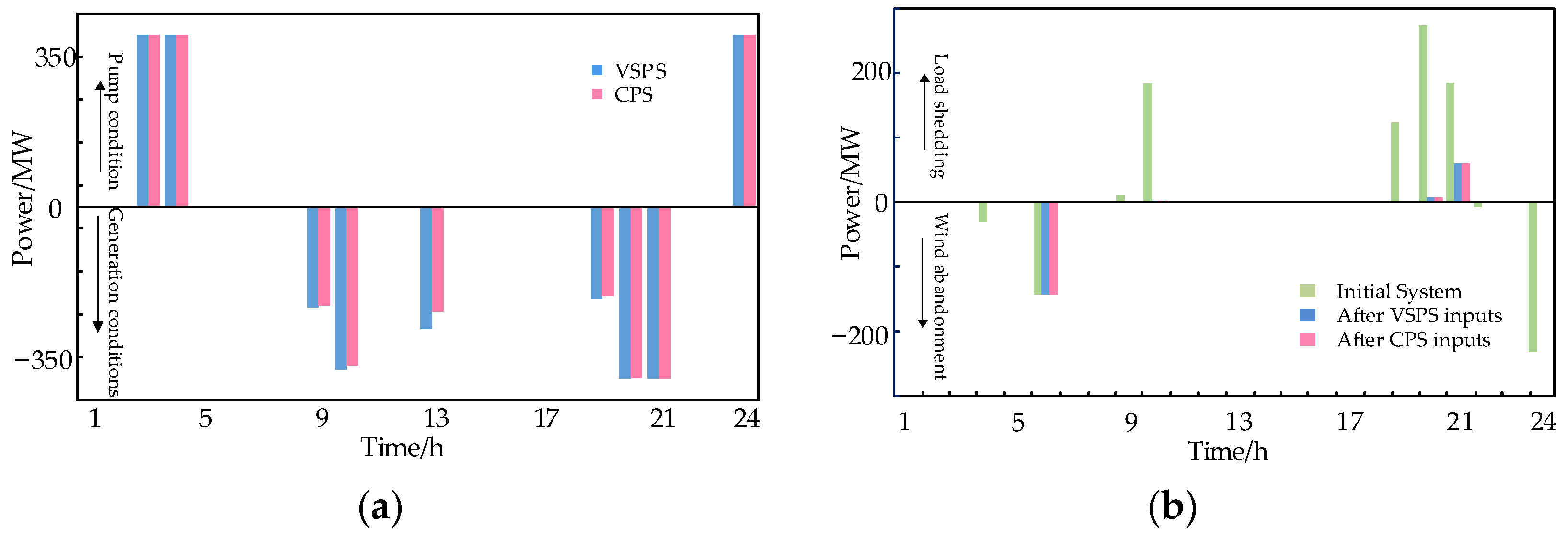
(1) Scenario 1: The new energy penetration rate is low, and the net load fluctuation is not large and the pumped storage unit capacity is large. The load forecast value is shown in Table A3 of Appendix A, and the optimization strategy analysis adopts the electricity tariffs, capacity tariffs, and other parameters related to the operating costs as shown in Table A4 of Appendix A. The VSPS and CPS units are set to have a rated power of 400 MW. The power efficiency relationship is shown in Appendix B, Equation (A1), and the operating constraints are shown in Appendix B, Equation (A2). Using the operation strategy optimization model established in this study, a comparison of the regulated power of the VSPS and CPS units in each time period and the change in system flexibility before and after the pumping units participate in flexibility regulating are shown in Figure 4.

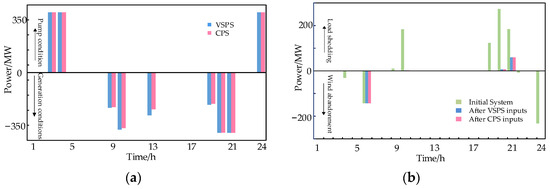
Figure 4. Results of Scenario 1. (a) Each hour of regulation power by the VSPS and CPS units, (b) wind abandonment or load cutting caused by insufficient flexibility before and after adjustment.

As shown in Figure 4b, the system before regulation has a more pronounced lack of downward flexibility in the 4th, 6th, 22nd, and 24th hours and a more pronounced lack of upward flexibility in the 9th, 10th, and 19th–21st hours. In addition, a small flexibility deficit is noted in the 2nd and 13th hours. With the VSPS or CPS units in operation, the degree of the system flexibility deficit was substantially reduced in all time periods except the 6th hour. Compared with starting operation in the 6th hour, the unit operates in the pumping condition in the 3rd–4th hours, and this is more favorable for the unit to output more energy in the subsequent hours by absorbing more power to balance the change in the unit’s stored energy and solving the load-shedding problem of the system due to the lack of flexibility. Due to the limitation of the maximum number of startups, the unit can only choose to participate in regulation during either the 3rd–4th hours or the 6th hour. Considering that if the unit participates in regulation during the 6th hour, although it solves the problem of wind abandonment caused by the lack of flexibility in that hour, the total amount of energy stored in the VSPS unit will be reduced, which is not conducive to the solution of the load-shedding problem due to the lack of flexibility in the subsequent hours. Therefore, the unit is selected to run in the pumping condition in the 3rd–4th hours and stop running in the 6th hour under the optimized operation strategy. It is worth noting that the comparison between the VSPS and CPS output curves is not significant due to the small net load fluctuations in this scenario and the wide range of adjustable settings for the pumped storage unit’s stored energy. However, from Figure 4b, it can be seen that when the units have the same value of output in the pumping condition, the VSPS unit is able to output more power in the generating condition due to its higher operational efficiency, which results in a larger system flexibility margin.

The total number of startups, shutdowns, and condition transitions; the increase in new energy consumption; the total amount of load-shedding reduction; the total number of time periods involved in regulation; and the changes in energy storage before and after scheduling during the operation of the VSPS and CPS units are shown in Table 1.

Table 1. Comparison of state parameters of the VSPS and CPS units participating in flexibility regulation.

System Operation Case	Participation of VSPS	Participation of CPS
Number of startups and shutdowns/times	5	5
Number of condition changes/times	2	2
Increase in new energy consumption/MW·h	271.18	271.18
Total reduction of load-slicing/MW·h	706.03	706.03
Total number of hours engaged in regulation/h	9	9
Energy storage after dispatch/MW·h	2999.97	3065.81
Rate of energy storage change before and after dispatch/%	25.00	23.35

As can be seen in Table 1, in the case of low penetration of new energy and a large capacity of pumped storage reservoirs, guiding the pumped storage to participate in the system flexibility regulation according to the scheme proposed in this study could maximize the amount of new energy consumption and reduce the load-cutting under the condition of meeting the constraints set for the operation. Moreover, the optimization scheme sets an upper limit on the rate of the total energy storage change before and after dispatch, which is able to constrain the energy storage change to prevent the dispatch from being affected in the next cycle.

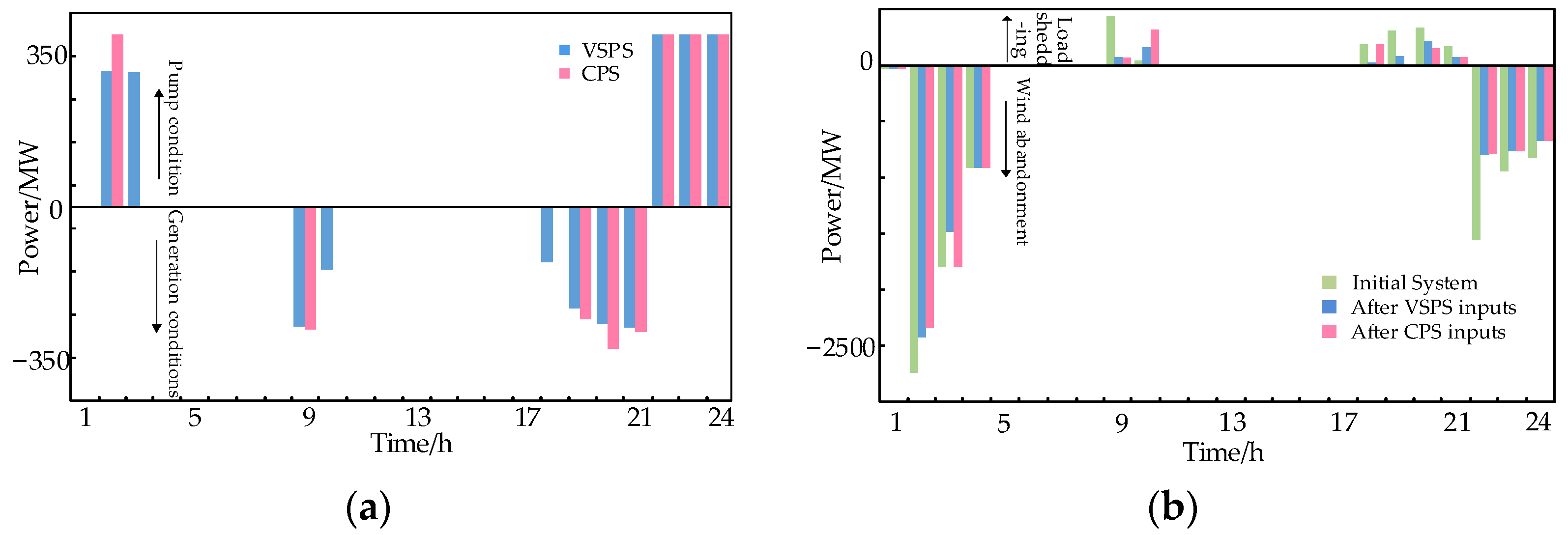
(2) Scenario 2: Assuming that the load forecast is the same as Scenario 1, the new energy output forecast is doubled, and the reservoir capacity of the pumped storage unit is smaller. The VSPS operating constraints are shown in Appendix B, Equation (A3). A comparison of the regulated power of the VSPS and CPS units in each time period and the change in system flexibility before and after the pumping units participate in flexibility regulation are shown in Figure 5.

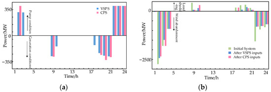
Figure 5. Results of Scenario 2. (a) Each hour of power regulation by the VSPS and CPS units, (b) wind abandonment or load cutting caused by insufficient flexibility before and after adjustment.

Comparison of Figure 4b and Figure 5b shows that the degree of system inflexibility increases significantly as new energy penetration increases. After the pumped storage unit’s reservoir capacity decreases, the difference between the regulated power of the VSPS and CPS units in each time period begins to appear. Given that the CPS unit can only operate at rated power in pumping condition, after the 2nd hour of operation, the remaining storage capacity is not sufficient to support the unit to continue to operate in the pumping condition in the 3rd hour. In contrast, the VSPS unit has a minimum operating power of 300 MW in the pumping condition, and the remaining storage capacity can support its continuous output in the 2nd–3rd hours. Therefore, although the VSPS is less effective than the CPS of regulating the flexibility deficiency in the 2nd hour, it is more effective in the 2nd–4th hours. Similarly, the VSPS unit is able to operate continuously in the generating condition during the 10th and 18th hours, while the CPS unit is not able to produce power during those hours due to the operating range limitation. Thus, the VSPS regulates the system’s flexibility more effectively during the corresponding hours. The operational benefits of VSPS and CPS participation in regulation as well as the total amount of wind abandonment and load shedding in the system due to lack of flexibility before and after regulation are shown in Table 1.

Although in Figure 5b shows that the CPS unit is better than the VSPS unit for system flexibility regulation in some time periods, the benefits of the VSPS unit’s participation in flexibility regulation to reduce the total system wind abandonment or load shedding demand as well as regulation are better than those of the CPS unit in the entire regulation cycle as can be seen in Table 2.

Table 2. Comparison of the effects of the VSPS and CPS units in flexibility regulation.

System Operation Scheme	Pre-Regulation	VSPS Participation	CPS Participation
Operational benefits CI/¥		578,419.98	545,066.49
Total wind abandonment and load shedding ΔCPSF/MW	10,290.827	7728.03	8116.40

The total number of startups, shutdowns and condition transitions; the increase in new energy consumption; the total amount of load-shedding reduction; the total number of time periods involved in regulation; and the changes in energy storage before and after scheduling during the operation of the VSPS and CPS units are shown in Table 3.

Table 3. Comparison of state parameters of the VSPS and CPS units participating in flexibility regulation.

System Operation Case	Participation of VSPS	Participation of CPS
Number of startups and shutdowns/times	4	4
Number of condition changes/times	2	2
Increase in new energy consumption/MW·h	1836.52	1777.74
Total reduction of load-slicing/MW·h	966.66	955.10
Total number of hours engaged in regulation/h	11	8
Energy storage after dispatch/MW·h	1779.59	1785.73
Rate of energy storage change before and after dispatch/%	19.11	18.83

As can be seen from Table 3, in the case of a high new energy penetration rate and small pumped storage capacity, guiding the pumped storage to participate in system flexibility regulation according to the scheme proposed in this study can utilize the advantages of the VSPS unit in the flexibility regulation process. Under the same starting and stopping times and the same number of working condition transitions, the VSPS unit can increase new energy consumption and reduce the total amount of load shedding to a greater extent in the scheduling cycle due to its wider operating range and higher efficiency.

5. Conclusions

In this study, starting from the realization of the VSPS unit to improve system flexibility and taking into account the operating efficiency of the unit, a method to quantify the system’s flexibility deficiency based on the probability density calculation considering the uncertainty of the source load is proposed, and the constraints to optimize the participation of the VSPS unit in the scheduling and operation are established. Then, an optimization method for the operation strategy of the VSPS unit is proposed to improve system flexibility. The following conclusions are drawn from the simulation study:

(1)

The proposed flexibility quantification method can reasonably quantitatively assess the total amount of the system’s flexibility deficit, which facilitates the construction of the objective function of the optimization model for improving system flexibility.

(2)

Increased penetration of new energy sources affects the degree of the system’s flexibility deficit, and the VSPS unit offers an advantage by participating in system flexibility regulation compared with the CPS unit.

At the same time, it is worth pointing out that the calculation process only considered the operating income of the VSPS unit itself; thus, comprehensive consideration of the influence of the total income on the operation strategy optimization is worthy of in-depth development. The next step of the study will consider using a more accurate model to fit the new energy error and construct parameters to correct the impact of the conventional thermal power unit output limitation on the optimization of VSPS unit operation due to economic factors to make the model established in this study more conducive for application to the system unit output planning for flexibility regulation.

References

- Rogelj, J.; Popp, A.; Calvin, K.V.; Luderer, G.; Emmerling, J.; Gernaat, D.; Fujimori, S.; Strefler, J.; Hasegawa, T.; Marangoni, G.; et al. Scenarios towards limiting global mean temperature increase below 1.5 °C. Nat. Clim. Chang. 2018, 8, 325–332. [Google Scholar] [CrossRef]
- Davis, S.J.; Lewis, N.S.; Shaner, M.; Aggarwal, S.; Arent, D.; Azevedo, I.L.; Benson, S.M.; Bradley, T.; Brouwer, J.; Chiang, Y.M.; et al. Net-zero emissions energy systems. Science 2018, 360, 9793. [Google Scholar] [CrossRef]
- Ding, N.; Duan, J.; Xue, S.; Zeng, M.; Shen, J. Overall review of peaking power in China: Status quo, barriers and solutions. Renew. Sustain. Energy Rev. 2015, 42, 503–516. [Google Scholar] [CrossRef]
- Gu, Y.; Xu, J.; Chen, D.; Wang, Z.; Li, Q. Overall review of peak shaving for coal-fired power units in China. Renew. Sustain. Energy Rev. 2016, 54, 723–731. [Google Scholar] [CrossRef]
- IEA. The Power of Transformation: Wind, Sun and the Economics of Flexible Power Systems; International Energy Agency: Paris, France, 2014. [Google Scholar]
- Tuohy, A.; O’Malley, M. Pumped storage in systems with very high wind penetration. Energy Policy 2011, 39, 1965–1974. [Google Scholar] [CrossRef]
- Attya, A.B.T.; Hartkopf, T. Utilising stored wind energy by hydro-pumped storage to provide frequency support at high levels of wind energy penetration. IET Gener. Transm. Distrib. 2015, 9, 1485–1497. [Google Scholar] [CrossRef]
- Khodayar, M.E.; Shahidehpour, M.; Wu, L. Enhancing the dispatchability of variable wind generation by coordination with pumped-storage hydro units in stochastic power system. IEEE Trans. Power Syst. 2013, 28, 2808–2818. [Google Scholar] [CrossRef]
- Hozouri, M.A.; Abbaspour, A.; Fotuhi-Friuzabad, M.; Moeini-Aghtaie, M. On the use of pumped storage for wind energy maximization in transmission-constrained power systems. IEEE Trans. Power Syst. 2015, 30, 1017–1025. [Google Scholar] [CrossRef]
- Zou, J.; Pipattanasomporn, M.; Rahman, S.; Lai, X. A Frequency Regulation Framework for Hydro Plants to Mitigate Wind Penetration Challenges. IEEE Trans. Sustain. Energy 2016, 7, 1583–1591. [Google Scholar] [CrossRef]
- Xia, S.; Ding, Z.; Du, T.; Zhang, D.; Shahidehpour, M.; Ding, T. Multi-time scale coordinated scheduling for the combined system of wind power, photovoltaic, thermal generator, hydro pumped storage, and batteries. IEEE Trans. Ind. Appl. 2020, 56, 2227–2237. [Google Scholar] [CrossRef]
- Basu, M. Multi-region dynamic economic dispatch of solar-wind-hydro-thermal power system incorporating pumped hydro energy storage. Eng. Appl. Artif. Intell. 2019, 86, 182–186. [Google Scholar] [CrossRef]
- Duque, A.J.; Castronuovo, E.D.; Sanchez, I.; Usaola, J. Optimal operation of a Pumped-storage hydro plant that compensates the imbalances of a wind power producer. Electr. Power Syst. Res. 2011, 81, 1767–1777. [Google Scholar] [CrossRef]
- Deane, J.P.; Ó Gallachóir, B.P.; McKeogh, E.J. Techno-economic review of existing and new pumped hydro energy storage plant. Renew. Sustain. Energy Rev. 2010, 14, 1293–1302. [Google Scholar] [CrossRef]
- Feng, C.; Zheng, Y.; Mai, Z.; Wu, W.; Chen, H. Cost advantage of adjustable-speed pumped storage unit for daily operation in distributed hybrid system. Renew. Energy 2021, 176, 1–10. [Google Scholar] [CrossRef]
- Mohanpurkar, M.; Ouroua, M.; Hovsapian, R.; Luo, Y.; Singh, M.; Muljadi, E.; Gevorgian, V.; Donalek, P. Real-time co-simulation of adjustable-speed pumped storage hydro for transient stability analysis. Electr. Power Syst. Res. 2018, 154, 276–286. [Google Scholar] [CrossRef]
- Chazarra, M.; Pérez-Díaz, J.I.; García-González, J. Optimal joint energy and secondary regulation reserve hourly scheduling of variable speed pumped storage hydropower plants. IEEE Trans. Power Syst. 2018, 33, 103–115. [Google Scholar] [CrossRef]
- Kougias, I.; Aggidis, G.; Avellan, F.; Deniz, S.; Lundin, U.; Moro, A.; Muntean, S.; Novara, D.; Pérez-Díaz, J.I.; Quaranta, E.; et al. Analysis of emerging technologies in the hydropower sector. Renew. Sustain. Energy Rev. 2019, 113, 109257. [Google Scholar] [CrossRef]
- Anupam, A.T.; Le, X. A metric and market construct of inter-temporal flexibility in time-coupled economic dispatch. IEEE Trans. Power Syst. 2016, 31, 3437–3446. [Google Scholar]
- Sutanto, D.; Outhred, H.R.; Lee, Y.B. Probabilistic power system production cost and reliability calculation by the Z-transform method. IEEE Trans. Energy Convers. 1989, 4, 559–565. [Google Scholar] [CrossRef]
- Hald, A. The early history of the cumulants and the Gram-Charlier series. Int. Stat. Rev. 2000, 68, 137–153. [Google Scholar]
- Zhao, J.; Oh, U.; Park, J.; Park, E.S.; Im, H.B.; Lee, K.Y.; Choi, J.S. A Review of World-wide Advanced Pumped Storage Hydropower Technologies. IFAC Pap. OnLine 2022, 55, 170–174. [Google Scholar] [CrossRef]
- Zhang, Z.; Cai, X.; Parkun, D. Determination of Pumped Storage Capacity Combining Entropy Weighting Method and Principal Component Analysis. J. Power Technol. 2014, 94, 165–175. [Google Scholar]
Disclaimer/Publisher’s Note: The statements, opinions and data contained in all publications are solely those of the individual author(s) and contributor(s) and not of MDPI and/or the editor(s). MDPI and/or the editor(s) disclaim responsibility for any injury to people or property resulting from any ideas, methods, instructions or products referred to in the content. |
© 2023 by the authors. Licensee MDPI, Basel, Switzerland. This article is an open access article distributed under the terms and conditions of the Creative Commons Attribution (CC BY) license (https://creativecommons.org/licenses/by/4.0/).