Efficient Strategies for Computing Euler Number of a 3D Binary Image

Abstract

As an important topological property for a 3D binary image, the Euler number can be computed by finding specific a voxel block with 2 × 2 × 2 voxels, named the voxel pattern, in the image. In this paper, we introduce three strategies for enhancing the efficiency of a voxel-pattern-based Euler number computing algorithm used for 3D binary images. The first strategy is taking advantage of the voxel information acquired during computation to avoid accessing voxels repeatedly. This can reduce the average number of accessed voxels from 8 to 4 for processing a voxel pattern. Therefore, the efficiency of computation will be improved. The second strategy is scanning every two rows and processing two voxel patterns simultaneously in each scan. In this strategy, only three voxels need to be accessed when a voxel pattern is processed. The last strategy is determining the voxel accessing order in the processing voxel pattern and unifying the processing of the voxel patterns that have identical Euler number increments to one group in the computation. Although this strategy can theoretically reduce the average number of voxels accessed from 8 to 4.25 for processing a voxel pattern, it is more efficient than the above two strategies for moderate- and high-density 3D binary images. Experimental results demonstrated that the three algorithms with each of our proposed three strategies exhibit greater efficiency compared to the conventional Euler number computing algorithm based on finding specific voxel patterns in the image.

1. Introduction

With the growth of digital images on the web and elsewhere, we need to search, retrieve and classify the images in many applications. Aimed at the problem of image search result organization, Ref. [1] provides a review of the popular methods related to cluster-based image search result organization. By these methods, color images can be categorized by visual features or text features. However, binary images are one of the important images in many image processing systems, and they are often classified by their topological properties. Topological properties of a binary image play a significant role in image recognition, object classification, image segmentation and many other analysis applications. For a binary image, the Euler number remains unchanged despite stretching, flexing or rotating the image, making it a valuable property in many image processing applications, such as medical diagnosis [2], object recognition based on reflectance [3] and crack detection [4]. Numerous algorithms for computing the Euler number of 2D binary images have been used in the past decades, which can be categorized into perimeter-based algorithms [5,6,7], bit-quad-based algorithms [8,9], run-based algorithms [10,11], graph-based algorithms [12,13] and labeling-based algorithms [14,15].

Recent advancements in image processing and analysis have led to an increase in demand for 3D image processing. The Euler number of 3D images is often used for characterizing complex microstructures [16,17]. For example, it can be used for differentiating the morphologies of graphite; thus, the growth mechanism and the properties of cast iron can be understood precisely.

The definition of Euler number in a 3D binary image is presented by Formula (1).

E = C – T + B

(1)

where C represents the number of connected components, T represents the number of tunnels (or holes), and B represents the number of bubbles (or cavities) in the given image [18,19].

For clarity and convenience, it should be noted that the term “image” henceforth refers exclusively to “binary image”.

In addition to this definition, many different kinds of algorithms have been introduced for obtaining the Euler number of 3D images. As introduced above, perimeters and contact perimeters have been used in calculating the Euler number in 2D cases [5,6,7]. Accordingly, Bribiesca extended it to 3D cases. Ref. [5] presented a perimeter-based algorithm that computes the Euler number of one-voxel-width 3D images according to the perimeters and contact perimeters involved in the connected components of the given image. Akira and Aizawa [20] used an n × n array of finite-state automata to calculate the numbers of connected components, holes and cavities in the given image, after which the Euler number can be obtained easily by use of Formula (1). Lee and Poston [21] presented an algorithm that smooths the given 3D image and applies theorems of differential geometry and algebraic topology. Moreover, Saha and Chaudhuri proposed an efficient method for obtaining the numbers of connected components, holes and cavities under a specific connectivity relation in [22,23] that can compute the Euler number of the given image using Formula (1). Additionally, Lin et al. introduced an algorithm for computing the Euler number of a 3D image by adding up the number of consecutive voxels, named runs, and adjacent runs existing in the given image [24,25]. This algorithm is extended from 2D cases. Meanwhile, Sánchez-Cruz et al. [26] proposed a new algorithm for computing the Euler number through analyzing the voxelized connected components with cavities and/or tunnels and the relationship between adjacent voxel faces with enclosing surfaces. The algorithm proposed in [26] counts specific voxel patterns, including 1 × 2 × 2, 2 × 1 × 2, 2 × 2 × 1, and 2 × 2 × 2, in the image. In the last few years, two distinctive methods have been presented for calculating the Euler number of a 3D image. Sossa [27] presented a codification-based algorithm that employs the codification of vertices of the foreground voxels in a given image. This algorithm can be thought of as the extension of the algorithm presented in [28]. Moreover, Čomića [29] presented a surface-based formula in computing the Euler number in 3D binary images. This algorithm involves counting only the boundary vertices and faces in the connected components, with the vertex count adjusted for the two adjacency relations.

In [18], Park and Rosenfeld proposed a simple algorithm for computing the Euler number in the given 3D image. This algorithm counts specific 2 × 2 × 2 voxel patterns for the six adjacent cases between voxels. As an extension, Morgenthaler solves the problem of 26-adjacent cases between voxels in [30]. The two algorithms introduced in [18,30] are simple and convenient in implementation.

As mentioned in [20], the judgement of holes is not as easy as that in 2D cases. For example, there are two types of holes. The first type is like the hole in a donut, which allows for string threading. The other type is the hole that can contain jam [21]. Thus, it will raise ambiguities sometimes. Therefore, using a voxel-pattern-based algorithm to compute the Euler number of the given 3D image becomes a relatively good choice. For convenience, this voxel-pattern-based algorithm, proposed by Morgenthaler [30], is denoted as the VP algorithm in our paper.

When computing the Euler number of 3D images, the VP algorithm must access eight voxels in the corresponding voxel pattern in order to determine whether the current voxel pattern applies. However, many voxels are accessed repeatedly in the computation. If the repeated accession can be avoided, the algorithm can become more efficient. Based this consideration, three efficiency strategies for enhancing the efficiency of the VP algorithm when computing the Euler number of the given 3D image are introduced in this paper. The first strategy is taking advantage of the information of voxels acquired from the previous processed 2 × 2 × 2 voxel pattern to avoid accessing voxels repeatedly. Then, it is possible to reduce the average number of accessed voxels required for processing a voxel pattern from 8 to 4. Thus, the computing efficiency can be improved. We implement this strategy using state transition; thus, the algorithm with this strategy is denoted as the ST algorithm in this paper. The second strategy is scanning every two rows and processing two voxel patterns simultaneously. By this strategy, only three voxels need to be accessed for processing a voxel pattern in our proposed algorithm. Because more rows are scanned simultaneously in this strategy, the algorithm with this strategy is denoted as the MR algorithm in this paper. The last strategy focuses on the accessing order when processing a voxel pattern. We change the accessing order of voxels when processing voxel patterns, and at the same time, the voxel patterns with identical Euler number increments are combined to the same group for processing. Theoretically, when we process a voxel pattern by this strategy, the reduction of the average number of accessed voxels would be decreased from 8 to 4.25, but it is more efficient for moderate- and high-density images. In this strategy, we change the voxel accessing orders when we process a voxel pattern; thus, the algorithm with this strategy is denoted as the CO algorithm in this paper. Experimental results demonstrated that the algorithms with our strategies exhibit greater efficiency in comparison to the VP algorithm.

The organization of the paper is as follows: we review the conventional voxel-pattern-based Euler number computing algorithm in Section 2 and present our strategies in Section 3. In Section 4, experiments are conducted on different resolutions and different densities of noise images for evaluating the efficiency of different strategies in comparison to the VP algorithm. We discuss the algorithms in Section 5, and we present concluding remarks in the last section.

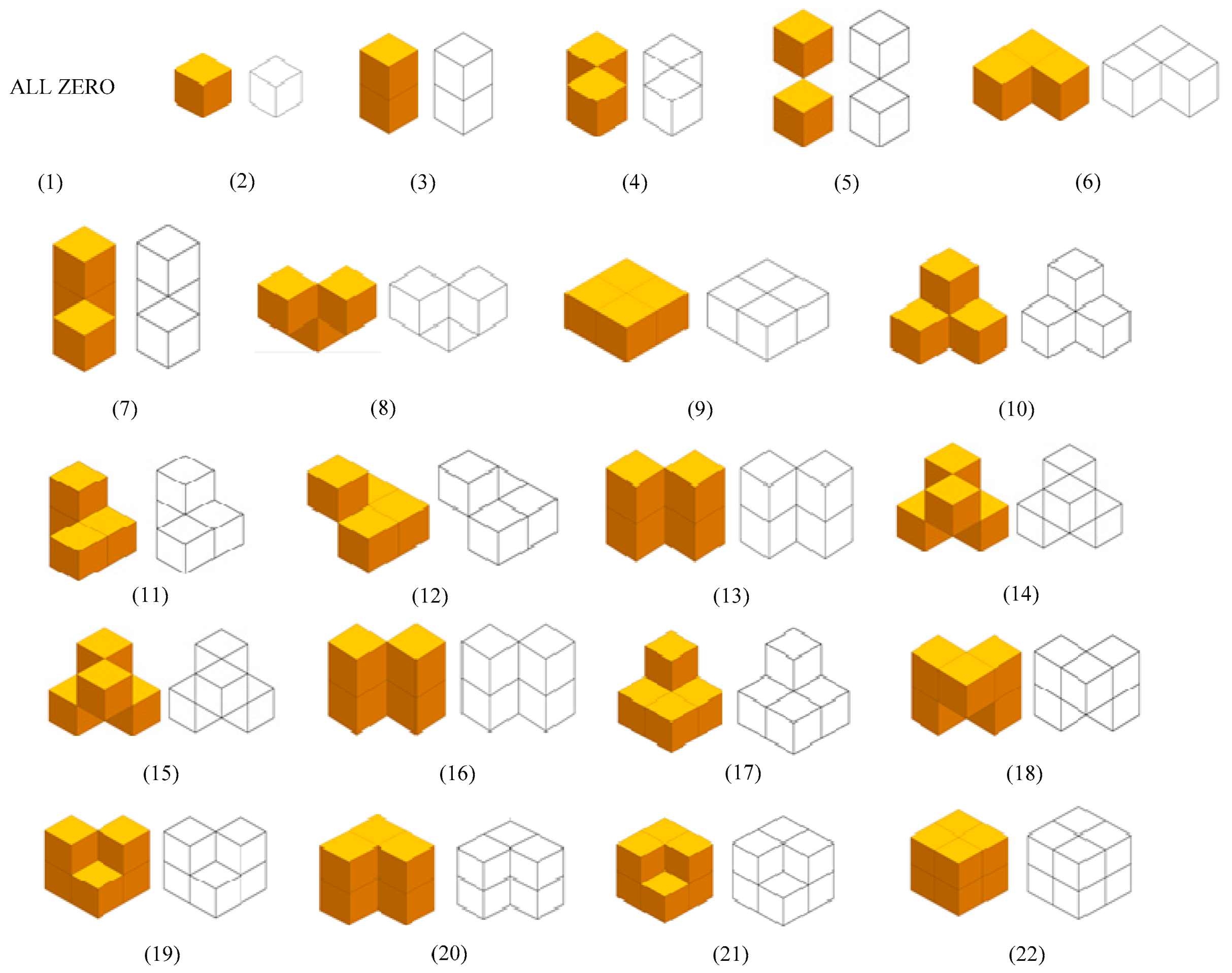
2. Reviews of Conventional Voxel-Pattern-Based Euler Number Computing Algorithm for a 3D Image

A 3D image can be described as an array of volume elements, or voxels. For the binary case, a 3D image can be considered as a relation or function f: Σ→{0, 1}, which maps from Σ to the set {0, 1}. To determine the adjacency between voxels in the image, a pair of voxels P = (a₁, a₂, a₃) and Q = (b₁, b₂, b₃) are considered to be 6-adjacent if their Manhattan distance is equal to 1, i.e., |a₁ − b₁| + |a₂ − b₂| + |a₃ − b₃| = 1. Alternatively, P and Q are considered to be 26-adjacent if their Chebyshev distance is equal to 1, i.e., max (|a₁ − b₁|, |a₂ − b₂|, |a₃ − b₃|) = 1. As illustrated in Figure 1, p₁, p₃, p₅, p₇, p₁₇ and p₂₆ are 6-adjacent to voxel p, and voxels p₁, p₂,…, p₂₆ are 26-adjacent to voxel p.

Figure 1. Illustration for explaining different adjacency among voxels.

We assume that the foreground voxels are expressed by 1 and the background voxels are expressed by 0 in a 3D image. Furthermore, all voxels on the border of the given image are assumed to be background voxels, which is the same as in most image processing algorithms. Additionally, only 26-adjacent between foreground voxels are considered in this paper.

In order to calculate the Euler number, specific configurations of 2 × 2 × 2 voxel patterns need to be found in the given image in the VP algorithm, as shown in Figure 2. Let #[x] (1 ≤ x ≤ 22) represents the number of occurrences that the voxel pattern i found in the given image, and then we can compute the Euler number according to Formula (2) [30].

E = Ψ₁ − Ψ₂ + Ψ₃ − Ψ₄ + Ψ₅ − Ψ₆ + Ψ₇ − Ψ₈

(2)

where

Figure 2. Different voxel patterns found in the algorithm proposed in [30].

• Ψ₁ = #[1];
• Ψ₂ = #[2] + #[3] + #[4];
• Ψ₃ = #[5] + #[6] + #[7];
• Ψ₄ = #[8] + #[9] + #[10] + #[11] + #[12] + #[13] + #[14];
• Ψ₅ = #[15] + #[16] + #[17];
• Ψ₆ = #[18] + #[19] + #[20];
• Ψ₇ = #[21];
• Ψ₈ = #[22].

In is known that a 2 × 2 × 2 voxel pattern consists of eight voxels, and each of them is either a foreground voxel or a background voxel. Accordingly, there will be 256 different types of configurations formed by the eight voxels, theoretically. To determine a voxel pattern’s configuration as found in the image, it is necessary to check it from all orientations. In practice, it is difficult to determine the voxel patterns’ configurations occurring in the image from all orientations. To address this issue, Morgenthaler summed up the Euler number increments of 256 different types of voxel patterns in the VP algorithm and listed their increments (see Table 1). The table lists the Euler number increment ΔE of voxel patterns that are not zero according to an index generated by the values of voxels in the voxel pattern. For instance, for the voxel pattern presented in Figure 3, if the values of voxels a, b, c, d, e, f, g and h are 1, 0, 1, 1, 1, 1, 1 and 1, respectively, the index should be 10111111, and from Table 1, it can be concluded that the Euler number increment of the current voxel pattern will be 1. In other words, once this pattern is found in the image, the Euler number of the image should be increased by 1. The Euler number increments of the other voxel patterns should be decided using a similar method.

Table 1. Voxel patterns’ indexes and their Euler number increments.

Index of Voxel Patterns	ΔE	Index of Voxel Patterns	ΔE	Index of Voxel Patterns	ΔE
00000010	1	00001001	−1	00001011	−1
00011000	−1	00011001	−1	00011010	−1
00011011	−1	00100001	−1	00100011	−1
00100100	−1	00100101	−1	00100110	−1
00100111	−1	00101000	−1	00101001	−2
00101010	−1	00101011	−2	00101100	−1
00101101	−1	00101110	−1	00101111	−1
00111000	−1	00111001	−1	00111010	−1
00111011	−1	10000001	−1	10000011	−1
10001001	−1	10001011	−1	10010100	1
10010101	1	10010110	1	10010111	1
10011100	1	10011101	1	10011110	1
10011111	1	10100001	−1	10100011	−1
10101001	−1	10101011	−1	10110100	1
10110101	1	10110110	1	10110111	1
10111100	1	10111101	1	10111110	1
10111111	1	Others	0

Figure 3. Distribution of voxels in a voxel pattern.

Although 256 different types voxel patterns can be formed by a 2 × 2 × 2 voxel block, as listed in Table 1, there are only 49 types of voxel patterns having non-zero Euler number increments. In other words, the increment of all the other 207 types of the voxel patterns is 0; thus, they will not have an influence on the Euler number of the image [30]. Among the voxel patterns which will have influences on the Euler number, 30 types of voxel patterns’ increments are −1, 17 types of voxel patterns’ increments are 1 and the last 2 types of voxel patterns’ increments are −2.

The VP algorithm is practicable in implementation. According to this algorithm, when computing the Euler number, it is necessary for us to access voxels in the image one by one, confirm the corresponding voxel patterns’ indexes and consult Table 1 for their Euler number increments. Once all voxels have been processed and all voxel patterns’ Euler number increments have been determined, we can obtain the Euler number of the given image easily. It is obvious that for finding the voxel patterns that will have influences on the Euler number, all voxel patterns’ Euler number increments have to be determined, and all the eight voxels have to be accessed in each voxel pattern. Therefore 8 × X × Y × Z voxel accessions are required for computing the Euler number of an image with a resolution of X × Y × Z voxels in the VP algorithm.

3. Our Proposed Strategies for Improving the VP Algorithm

As introduced above, while calculating the Euler number, for each voxel found in the raster scan, the VP algorithm will access all voxels in the corresponding voxel pattern when confirming whether the voxel pattern should be applied. As a matter of fact, plenty of voxels are accessed repeatedly in the computing procedure. In this section, we will introduce some strategies for reducing the number of voxel accessions while processing a voxel pattern.

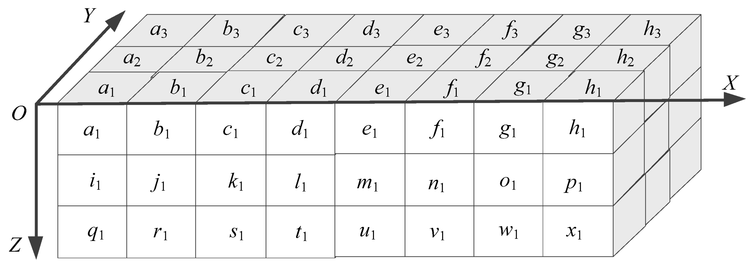
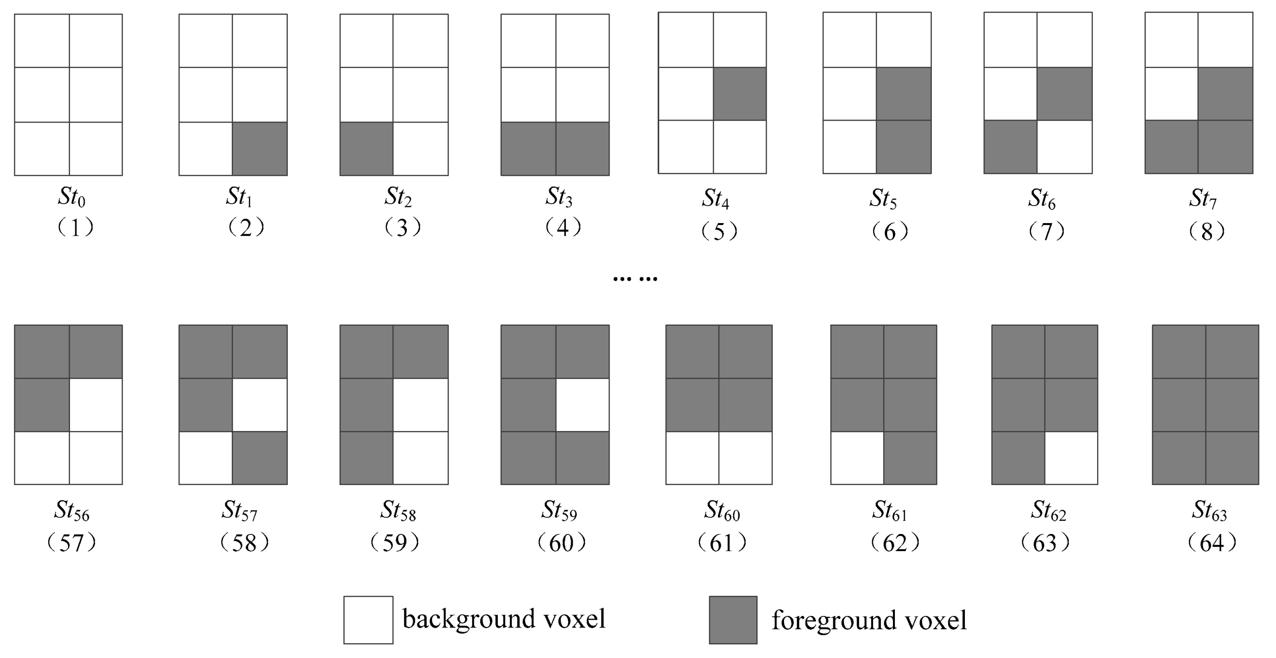
3.1. Strategy of State Transition

In the VP algorithm, many voxels would be accessed repeatedly. For example, as shown in Figure 4, when processing voxel a₁, it is required to access eight voxels in the corresponding voxel pattern {a₁, b₁, i₁, j₁, a₂, b₂, i₂, j₂} and confirm its index of the pattern. After doing this, it goes on to process the next voxel, i.e., voxel b₁, and the same method is used as in processing voxel a₁: eight voxels in the corresponding voxel pattern {b₁, c₁, j₁, k₁, b₂, c₂, j₂, k₂} will be accessed, where the voxels b₁, j₁, b₂ and j₂ have already been accessed while processing the previous voxel a₁. To prevent the repeated accesses, we can utilize the information of voxels b₁, j₁, b₂ and j₂ obtained during processing the voxel a₁.

Figure 4. Illustration of the repeated accessing of voxels existing in the VP algorithm.

In order to reduce the accession of voxels considered above, we construct sixteen different states for a quad, which are denoted as St₀, St₁, …, St₁₅, as shown in Figure 5. In this way, the left quad (four voxels) in the voxel pattern being processed can be replaced by the corresponding state, and thus, by utilizing transitions among the states, we only need to access the four voxels in the right quad in the current voxel pattern. Then, we describe the strategy in detail.

Figure 5. Sixteen states defined in the strategy of state transition.

Because all voxels on the border in a 3D image are considered to be background voxels, the left quad of the first voxel pattern will be the state St₀. Thus, we will begin our processing based on the state St₀ and access the other four voxels in the right quad for determining the index of the first voxel pattern of the image. For example, when the left quad of the current voxel pattern {a₁, b₁, i₁, j₁, a₂, b₂, i₂, j₂}, i.e., {a₂, a₁, i₂, i₁}, shown in Figure 4, is the case St₀, we only need to access the voxels in the right quad {b₂, b₁, j₂, j₁} for determining the index of the voxel pattern. After doing this, we proceed to process the following voxel pattern {b₁, c₁, j₁, k₁, b₂, c₂, j₂, k₂}, where the left quad is {b₂, b₁, j₂, j₁}, which will be a certain state as listed in Figure 5 according to the values of voxels b₂, b₁, j₂ and j₁. Therefore, we only need to access the four voxels in the right quad {c₂, c₁, k₂, k₁}.

Then, let us consider, when the left quad {b₂, b₁, j₂, j₁} is, for example, the state St₇, i.e., {0, 1, 1, 1}, how to process the voxel pattern {b₁, c₁, j₁, k₁, b₂, c₂, j₂, k₂}. We first check the voxels in the right quad {c₂, c₁, k₂, k₁} to confirm its state. For each possible state St_i (0 ≤ i ≤ 15), we go a step further to determine the Euler number increment of the current voxel pattern by consulting Table 1. Then, let us consider some cases.

(1) If the values of voxels c₂, c₁, k₂ and k₁ are 0, as shown in Figure 4, the voxel pattern being processed will be {0, 0, 1, 0, 1, 0, 1, 0}. According to Table 1, we know that the current voxel pattern needs to be involved in the computation, and its Euler number increment is −1. Thus, the Euler number of the given image will decrease by 1. After doing this, we proceed to process the next one in the image. Because the values of voxels c₂, c₁, k₂ and k₁ are 0, we will process the next one from state St₀.

(2) If the values of voxels c₂, c₁, k₂ and k₁ are 0, 0, 0 and 1, respectively, the voxel pattern being processed will be {0, 0, 1, 0, 1, 0, 1, 1}. According to Table 1, we know that the current voxel pattern needs to be involved in the computation, and its Euler number increment is −2. Therefore, the Euler number will decrease by 2. After doing this, we proceed to process the next one in the image. Because the values of voxels c₂, c₁, k₂ and k₁ are 0, 0, 0 and 1, we will process the next one from state St₁.

(3) If the values of voxels c₂, c₁, k₂ and k₁ are 0, 1, 1 and 0, respectively, the voxel pattern being processed will be {0, 0, 1, 1, 1, 1, 1, 0}. According to Table 1, we know that the current voxel pattern does not need to be involved in the computation on account of its zero Euler number increment, and this voxel pattern will not have an influence on the Euler number of the image. Then we proceed to process the next voxel pattern. Because the values of voxels c₂, c₁, k₂ and k₁ are 0, 1, 1 and 0, we will process the next one from state St₆.

Similar procedures can be applied to process other cases. The processing results are presented in Table 2.

Table 2. The Euler number increment of a voxel pattern whose left quad is St₇.

The State of the Right Quad	Index	ΔE	The State of the Right Quad	Index	ΔE
St0	00101010	−1	St8	01101010	0
St1	00101011	−2	St9	01101011	0
St2	00101110	−1	St10	01101110	0
St3	00101111	−1	St11	01101111	0
St4	00111010	−1	St12	01111010	0
St5	00111011	−2	St13	01111011	0
St6	00111110	0	St14	01111110	0
St7	00111111	0	St15	01111111	0

For each of the other states of the left quad in the voxel pattern, we can process the voxel pattern in a similar way. This procedure will be executed recursively until we finish processing all voxel patterns. Thus, we acquire the indexes and the same increments of all voxel patterns as in the VP algorithm. Consequently, the Euler number of the given image can be obtained according to the increments of different voxel patterns easily.

In this strategy, taking advantage of the voxel information acquired while processing the previous voxels, the number of accessed voxels decreased from 8 to 4 while processing each voxel pattern, which is half of that in the VP algorithm. Thus, it results in more efficient computing. For convenience, the state-transition-based algorithm described above is denoted as the ST algorithm in this paper.

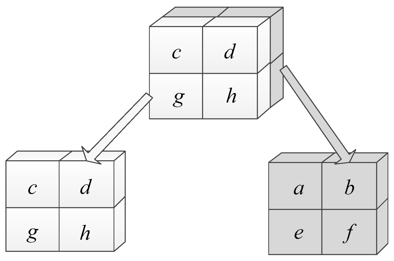
3.2. Scanning Every Two Rows and Processing Two Voxel Patterns Simultaneously

As introduced above, when processing a voxel pattern, the ST algorithm can avoid accessing the four voxels that have been accessed by making use of the voxel information acquired while processing the previous voxels. Nevertheless, many voxels are still accessed repeatedly in the ST algorithm. As shown in Figure 4, for processing the voxel a₁ in the first row, eight voxels in the voxel pattern {a₁, b₁, i₁, j₁, a₂, b₂, i₂, j₂} need to be accessed. Then, when we process the voxel i₁ in the next row, another eight voxels in the voxel pattern {i₁, j₁, q₁, r₁, i₂, j₂, q₂, r₂} need to be accessed. Obviously, voxels i₁, j₁, i₂ and j₂ will be accessed repeatedly.

We can avoid accessing such voxels repeatedly if we scan every two rows simultaneously, and for each voxel being processed, we access the involved twelve voxels to determine the indexes of two voxel patterns simultaneously. For example, when processing voxel a₁ in Figure 4, we access twelve voxels simultaneously, i.e., a₁, b₁, i₁, j₁, q₁, r₁, a₂, b₂, i₂, j₂, q₂ and r₂, to determine the indexes of two voxel patterns {a₁, b₁, i₁, j₁, a₂, b₂, i₂, j₂} and {i₁, j₁, q₁, r₁, i₂, j₂, q₂, r₂} simultaneously. For convenience, we represent the two voxel patterns as VP₁ and VP₂, respectively.

Furthermore, when we access twelve voxels to process two voxel patterns simultaneously, similar to that in the ST algorithm, by use of states transitions, we only need to access the voxels b₁, j₁, r₁, b₂, j₂, and r₂. Obviously, there are 2⁶ = 64 states, as shown in Figure 6, to be defined.

Figure 6. Sixty-four states defined in processing three rows simultaneously.

Similar to that in the ST algorithm, because all voxels on the border of a 3D image are background voxels, our computation should begin from state St₀, as shown in Figure 6(1), and access the other six voxels to determine the indexes of voxel patterns. As shown in Figure 4, when we process the first voxel a₁, because voxels a₂, a₁, i₂, i₁, q₂ and q₁ on the border are background voxels and the corresponding state is the state St₀, we only need to access voxels b₂, b₁, j₂, j₁, r₂ and r₁ to determine the indexes of voxel patterns {a₂, a₁, i₂, i₁, b₂, b₁, j₂, j₁} and {i₂, i₁, q₂, q₁, j₂, j₁, r₂, r₁}, respectively. After doing this, taking advantage of the state determined by the values of voxels b₂, b₁, j₂, j₁, r₂ and r₁, we go on to access the next six voxels c₂, c₁, k₂, k₁, s₂ and s₁ to confirm the indexes of voxel patterns {b₂, b₁, j₂, j₁, c₂, c₁, k₂, k₁} and {j₂, j₁, r₂, r₁, k₂, k₁, s₂, s₁}, respectively.

Then, let us consider, when the left six voxels {b₂, b₁, j₂, j₁, r₂, r₁} are, for example, the state St₇, i.e., {0, 0, 0, 1, 1, 1}, how to process the voxel patterns {b₁, c₁, j₁, k₁, b₂, c₂, j₂, k₂} and {j₂, j₁, r₂, r₁, k₂, k₁, s₂, s₁}. We first check the six voxels to the right of the twelve voxels, i.e., {c₂, c₁, k₂, k₁, s₂, s₁} to confirm its state St_i (0 ≤ i ≤ 63). Then, by using of two voxel patterns derived from the twelve voxels, we further confirm the Euler number increment of the corresponding voxel pattern by referring to Table 1. We use the following cases for explanation.

(1) If the values of voxels c₂, c₁, k₂, k₁, s₂ and s₁ are 0, 0, 0, 0, 0 and 0, respectively, then VP₁ will be {0, 0, 0, 0, 0, 0, 1, 0} and VP₂ will be {0, 0, 1, 0, 1, 0, 1, 0}. According to Table 1, we know that VP₁ should be involved in the computation, and its Euler number increment is 1. At the same time, VP₂ should be also involved, and its Euler number increment is −1. Then we proceed to process the next voxel pattern. Because the values of voxels c₂, c₁, k₂, k₁, s₂ and s₁ are 0, 0, 0, 0, 0 and 0, we will process the next one from state St₀.

(2) If the values of voxels c₂, c₁, k₂, k₁, s₂ and s₁ are 0, 0, 0, 0, 1 and 1, respectively, then VP₁ will be {0, 0, 0, 0, 0, 0, 1, 0} and VP₂ will be {0, 0, 1, 0, 1, 1, 1, 1}. According to Table 1, we know that VP₁ should be involved in the computation, and its Euler number increment is 1. However, VP₂ should not be involved because its Euler number increment is 0. Then we proceed to process the next voxel pattern. Because the values of voxels c₂, c₁, k₂, k₁, s₂ and s₁ are 0, 0, 0, 0, 1 and 1, we will process the next one from state St₃.

(3) If the values of voxels c₂, c₁, k₂, k₁, s₂ and s₁ are 1, 1, 1, 1, 1 and 1, respectively, then VP₁ will be {0, 1, 0, 1, 0, 1, 1, 1} and VP₂ will be {0, 1, 1, 1, 1, 1, 1, 1}. According to Table 1, we know that both VP₁ and VP₂ should not be involved in the computation because their Euler number increments are 0. Then, we proceed to process the next voxel pattern. Because the values of voxels c₂, c₁, k₂, k₁, s₂ and s₁ are 1, 1, 1, 1, 1 and 1, we will process the next one from state St₆₃.

Similar procedures can be applied to process other cases. The processing results are presented in Table 3.

Table 3. The Euler number increment of a voxel pattern whose left six voxels are St₇.

State of Right Voxels	Voxel Pattern	Index	ΔE	State of Right Voxels	Voxel Pattern	Index	ΔE
St0	VP1	00000010	1	St1	VP1	00000010	1
	VP2	00101010	−1		VP2	00101011	−2
St2	VP1	00000010	1	St3	VP1	00000010	1
	VP2	00101110	−1		VP2	00101111	−1
St4	VP1	00000011	0	St5	VP1	00000011	0
	VP2	00111010	−1		VP2	00111011	−1
St6	VP1	00000011	0	St7	VP1	00000011	0
	VP2	00111110	0		VP2	00111111	0
		……				……
		……				……
St56	VP1	01010110	0	St57	VP1	01010110	0
	VP2	01101010	0		VP2	01101011	0
St58	VP1	01010110	0	St59	VP1	01010110	0
	VP2	01101110	0		VP2	01101111	0
St60	VP1	01010111	0	St61	VP1	01010111	0
	VP2	01111010	0		VP2	01111011	0
St62	VP1	01010111	0	St63	VP1	01010111	0
	VP2	01111110	0		VP2	01111111	0

After all voxel patterns are processed in the image, we can acquire the same increments of all voxel patterns as in the VP algorithm. Thus, the Euler number of the image can be obtained easily on the basis of increments of different voxel patterns.

In this strategy, we scan every two image rows, and for each voxel in processing, we access six voxels to process two voxel patterns simultaneously. That is to say, for processing a voxel pattern, the average number of voxels needing to be accessed will be 6/2 = 3, which is fewer than that in the ST algorithm; thus, it might lead to more efficient processing. For convenience, this multi-row-scan-based algorithm is denoted as the MR algorithm in this paper.

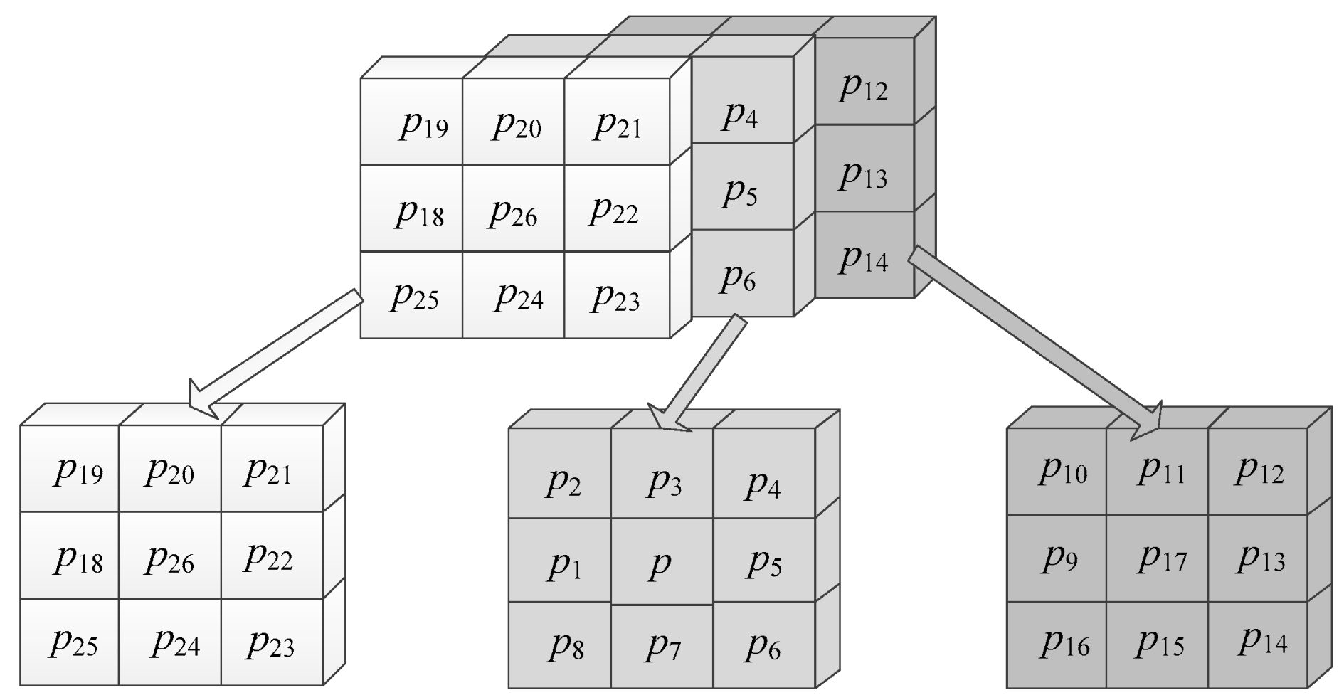
3.3. Strategy of Changing the Order of Accessing Voxels and Combining Similar Voxel Patterns

We continue to analyze the information in Table 1. It is not difficult to find that some voxel patterns’ indexes are consecutive, as listed in Table 4. Moreover, we can observe that these voxel patterns with consecutive indexes have something in common, i.e., these voxel patterns have the same Euler number increments. Accordingly, we can divide these voxel patterns into some groups. For example, for each voxel pattern indexed by 00011000, 00011001, 00011010 or 00011011 occurring in the processing, the Euler number will decrease by 1. On the other hand, it can be noticed that these consecutive indexes are different in the last two bits, which vary from 00 to 11.

Table 4. Euler number increments of voxel patterns with consecutive indexes.

Indexes of Voxel Patterns	ΔE	Indexes of Voxel Patterns	ΔE
00011000–00011011	−1	10010100–10010111	1
00100100–00100111	−1	10011100–10011111	1
00101100–00101111	−1	10110100–10110111	1
00111000–00111011	−1	10111100–10111111	1

Then, if the voxel patterns in each group are considered to be a voxel pattern cluster, we can represent the cluster by the first six voxels. In other words, the Euler number increments of the voxel patterns in these clusters can be acquired by accessing the first six voxels. For example, for the processing voxel pattern, if the values of the first six voxels a, b, c, d, e and f are 1, 0, 1, 1, 1 and 1, respectively, according to Table 4, we can deduce that the Euler number increment of the current voxel pattern is 1. In this case, we can acquire its Euler number increment without accessing voxel g and voxel h. Obviously, for processing a voxel pattern listed in Table 4, only six voxels need to be accessed.

By taking into account the aforementioned consideration, we can apply the same approach to the other groups of voxel patterns listed in Table 4. As shown in Table 4, 32 types of voxel patterns’ Euler number increments can be determined by the voxel information of the six voxels. Thus, this strategy will result in a more efficient computation.

We conducted further analysis on the voxel pattern indexes that have influences on the Euler number of the given image. An important observation was that the voxel located at the position “b” in each of these indexes is always a background voxel. Based on this observation, when we process a voxel pattern, we should focus on the voxel at the position “b” first. When the voxel “b” is found to be a background voxel, then we have to access other voxels in the voxel pattern for determining the increment. When the voxel “b” is found to be a foreground voxel, no voxels need to be accessed further, because the current voxel pattern Euler number increment must be 0. By this means, while processing a voxel pattern with a foreground voxel at the position “b”, only one voxel needs to be accessed for determining its Euler number increment.

In implementation, the two methods described above can be combined for improving the VP algorithm, and we can process a voxel pattern according to the following steps.

When processing the voxel pattern {a, b, c, d, e, f, g, h}, we first access the voxel “b” in its index.

(1) If the voxel “b” is a foreground voxel, it can be confirmed that the current voxel pattern does not need to be involved in the computation because its Euler number increment must be 0. Subsequently, we proceed to process the next one. In this case, only one voxel needs to be accessed for determining these voxel patterns’ Euler number increments.

(2) If the voxel “b” is a background voxel, we must conduct a sequential accessing of the voxels a, c, d, e and f of the current voxel pattern. If the values of voxels a, c, d, e and f are equal to one of the value groups {0, 0, 1, 1, 0}, {0, 1, 0, 0, 1}, {0, 1, 0, 1, 1}, {0, 1, 1, 1, 0}, {1, 0, 1, 0, 1}, {1, 0, 1, 1, 1}, {1, 1, 1, 0, 1} or {1, 1, 1, 1, 1}, following the list in Table 4, only six voxels need to be accessed for determining these voxel patterns’ Euler number increments.

(3) Otherwise, the two remaining voxels need to be accessed for determining the Euler number increment of the current voxel pattern. In this case, eight voxels need to be accessed for determining the Euler number increment.

By utilizing the above steps, we can process all voxel patterns in the given image and acquire the increments of all voxel patterns. Accordingly, the Euler number of the given image can be obtained easily. In this strategy, we change the accessing order of voxel patterns. For convenience, this changing-order-based algorithm is denoted as the CO algorithm in this paper.

4. Experimental Results

In this section, experiments are conducted on different resolutions of noise images for verifying the efficiency of different strategies in comparison to the VP algorithm. The performance of the ST algorithm, the MR algorithm and the CO algorithm will be compared with the VP algorithm. The efficiency of the algorithms is evaluated by their execution time in processing the same 3D images. All of the algorithms used for comparison were implemented in C language. The experimental environment and the experimental platform are presented in Table 5.

Table 5. The experimental setup and configurations of hardware and software.

Name	Version
Processor	Intel Core i7-6770
Frequency	3.20 GHz
Memory	8 GB
Operating System	Ubuntu Linux 20.04.1
GCC Compiler	4.6.1

Because noise images have random voxel distribution and complex connectivity among voxels, they are conducive to evaluating the performance of the algorithms. In our experiments, five resolutions (32 × 32 × 32, 64 × 64 × 64, 128 × 128 × 128, 256 × 256 × 256, 512 × 512 × 512 voxels) of 3D noise images were tested. For each resolution, 41 noise images were generated by thresholding of the images containing uniform random noise with 41 different values from 0 to 1000 in steps of 25. We presented nine cross sections of 3D noise images with densities of 0.1 to 0.9 in steps of 0.1 in Figure 7. In order to make the experimental results more accurate, we repeated the test 1000 times and obtained the experimental results by averaging of the execution time of the compared algorithms.

Figure 7. Crossing sections of noise images with different densities.

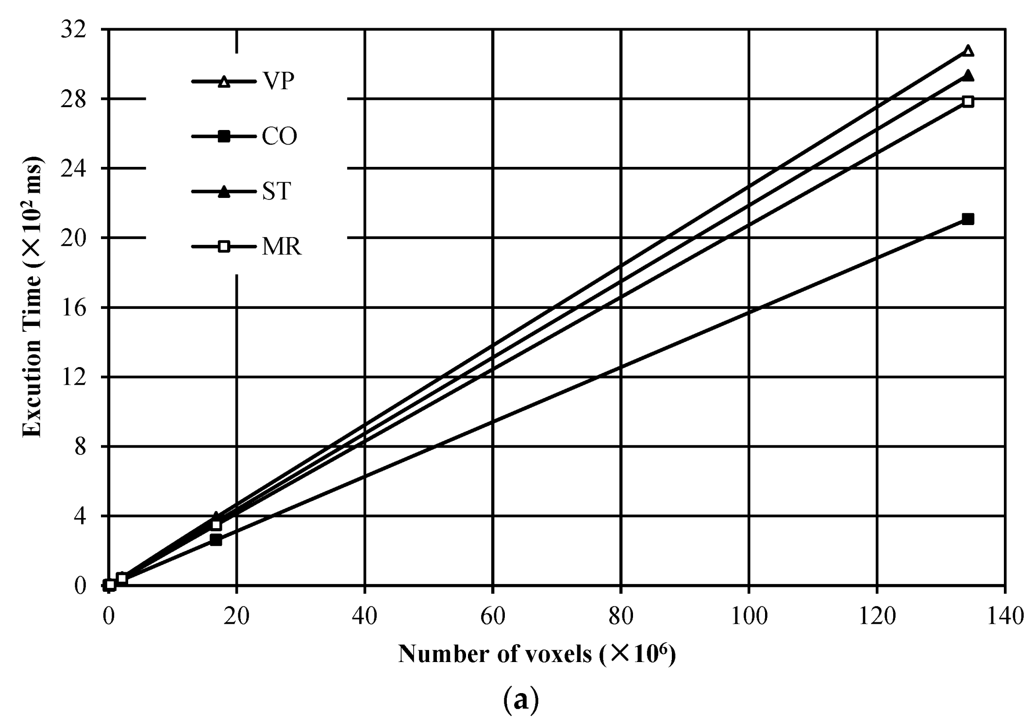
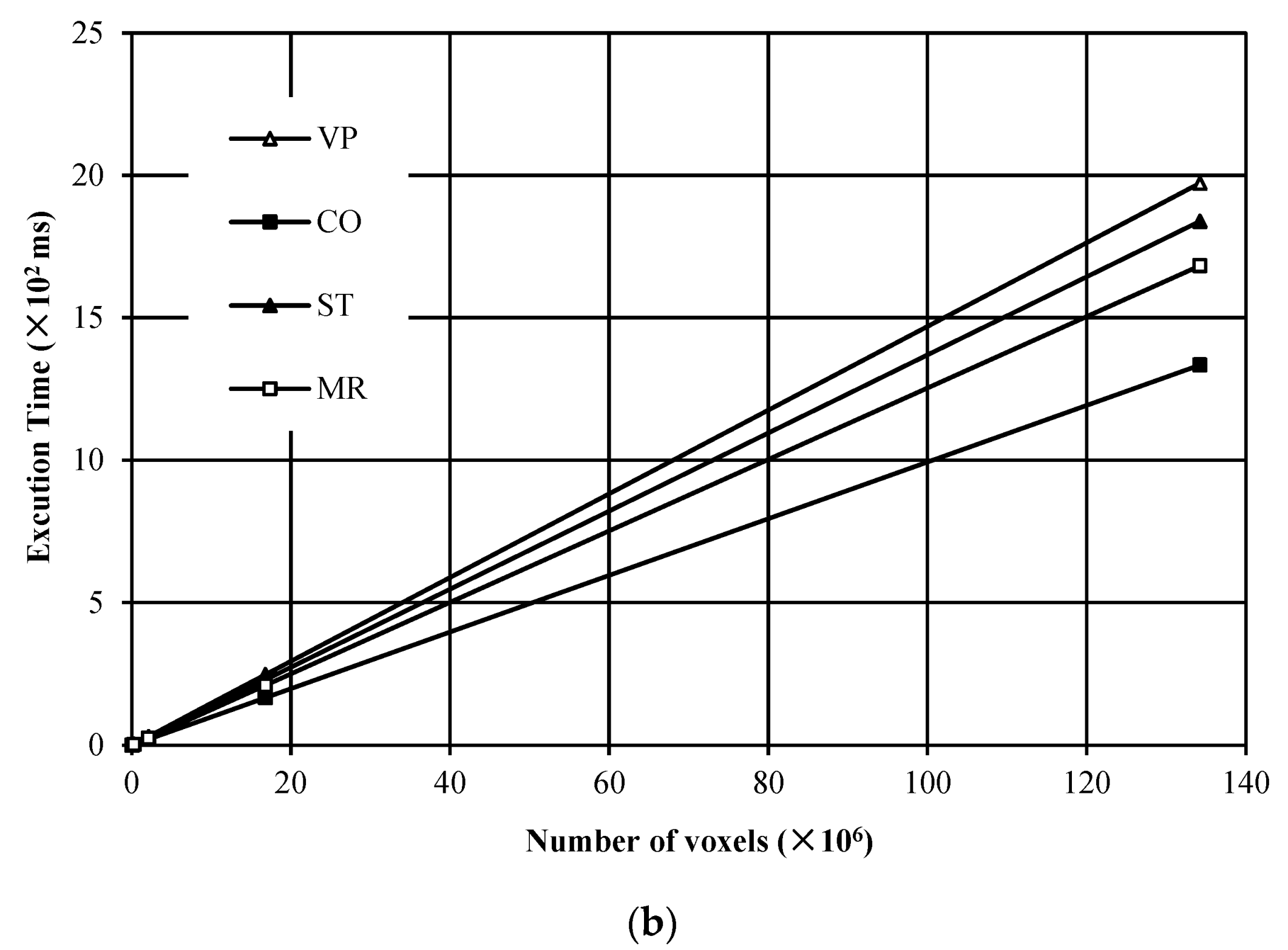
4.1. Execution Time versus the Number of Voxels in the Image

In this experiment, a total of 205 noise images with different resolutions were tested for evaluating the execution time versus the number of voxels for the compared algorithms. The experimental results are given in Figure 8. From Figure 8, it is found that for both the maximum execution time and the average execution time, all algorithms in comparison hold good linear features versus the number of voxels in the image. Furthermore, the algorithms with our proposed strategies perform more efficiently than the VP algorithm. Among the algorithms with our proposed strategies, the CO algorithm is the most efficient.

Figure 8. Execution time versus the number of voxels in the image: (a) the maximum execution time; (b) the average execution time.

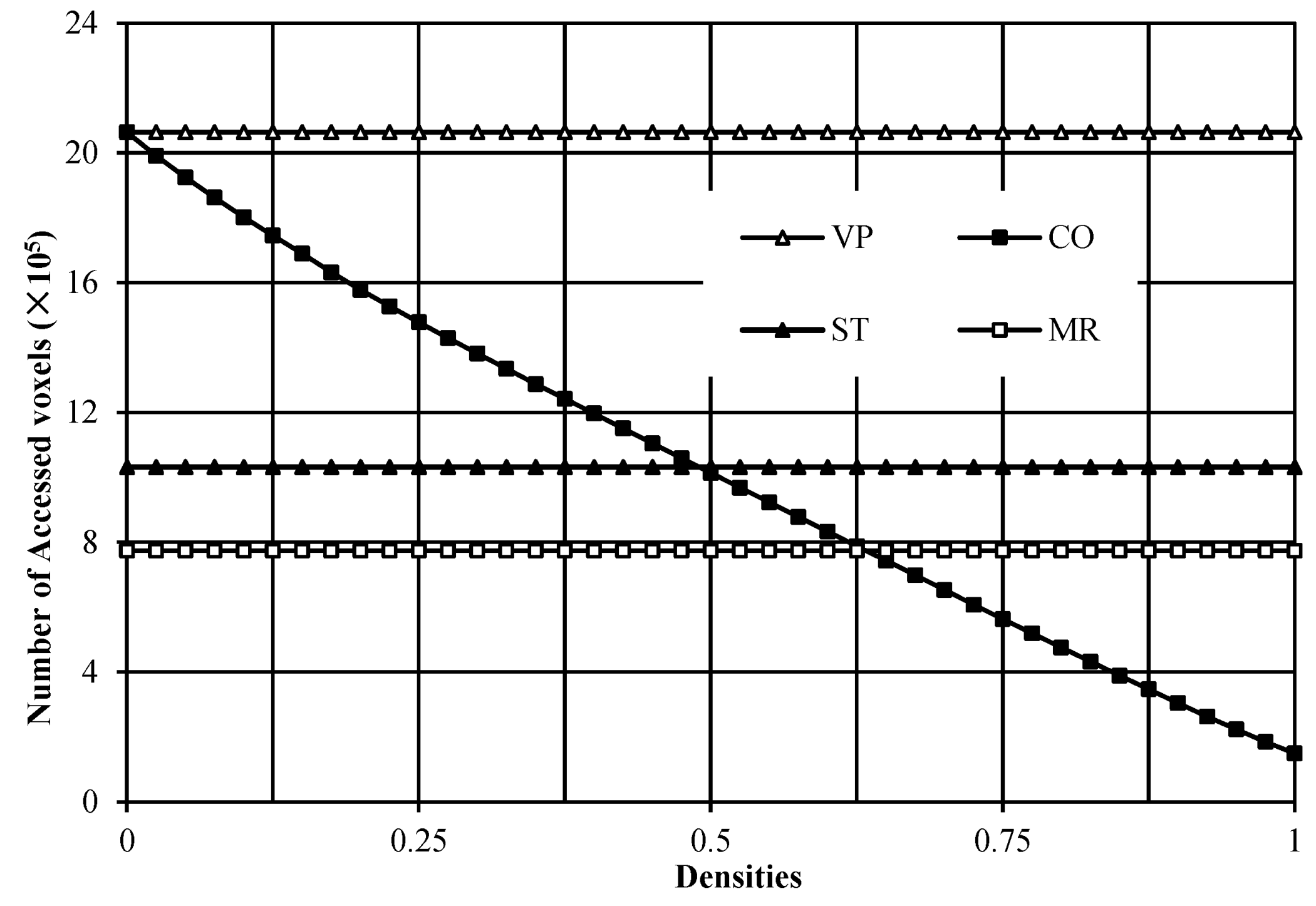
4.2. Comparison of the Number of Accessed Voxels in the Compared Algorithms

In this experiment, 41 noise images with a resolution of 64 × 64 × 64 voxels were tested for comparing the number of accessed voxels among the compared algorithms. The experimental results are shown in Figure 9. From Figure 9, it can be found that when all voxels are background voxels in the image, the number of accessed voxels in the VP algorithm is the same as that in the CO algorithm. With the increased densities of the foreground voxels in the images, the number of voxels needing to be accessed in the CO algorithm gradually becomes fewer than that in the VP algorithm. When all voxels are foreground voxels in the image, the number of voxels needing to be accessed in the CO algorithm is less than 1/10 of that in the VP algorithm. Moreover, for all tested images, the VP algorithm needs to access the same number of voxels. Similarly, the ST algorithm needs to access the same number of voxels for processing any image, but the number of accessed voxels is about half of that in the VP algorithm. As to the MR algorithm, for processing any image, it also needs to access the same number of voxels, which are fewer than that in the ST algorithm. This is consistent with our analysis.

Figure 9. Number of accessed voxels in the compared algorithms.

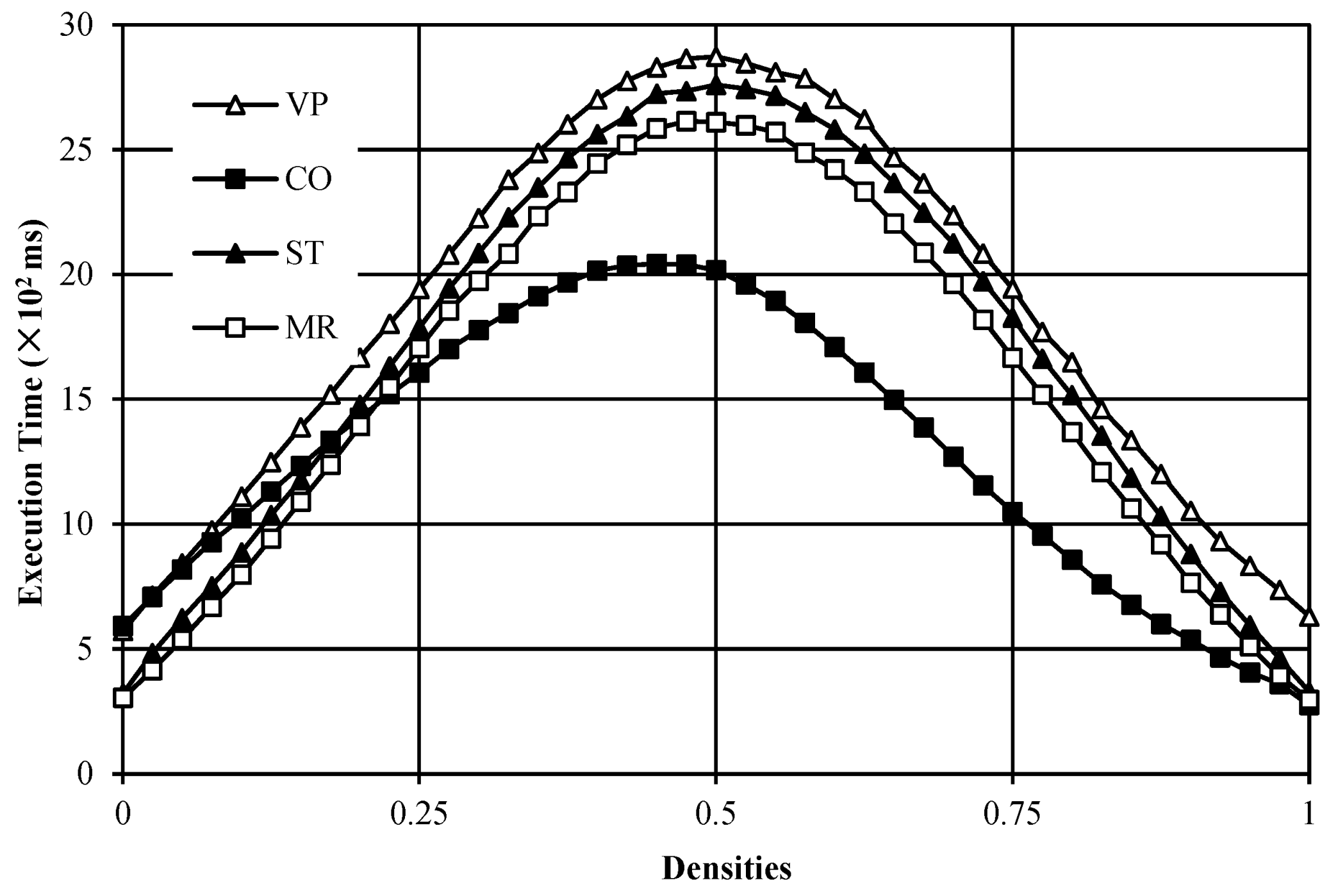
4.3. Execution Time versus Image Densities

In this experiment, 41 noise images with a resolution of 512 × 512 × 512 voxels are employed for verifying the execution time versus the densities of foreground voxels in the image. Figure 10 presents the trend of execution time of the compared algorithms. From Figure 10, it is found that the algorithms with our presented strategies are more efficient than the VP algorithm for almost all images.

Figure 10. Execution time versus image densities of foreground voxels.

Furthermore, as depicted above, for processing a voxel pattern, the number of voxels accessed in the ST algorithm and the MR algorithm is fewer than that in the VP algorithm. Therefore, the ST algorithm and the MR algorithm outperformed the VP algorithm. However, although the ST algorithm only accesses half of the number of voxels that the VP algorithm does, when we calculate the Euler number of a 3D image, the execution time of the ST algorithm is not half of that of the VP algorithm. Moreover, for all tested images, although the MR algorithm performs more efficiently than the ST algorithm, the difference between the two algorithms is minimal.

As to the CO algorithm, it is much more efficient than the other compared algorithms, in particular for those images whose densities of foreground voxels vary from 0.4 to 0.8. However, it is less efficient than the ST algorithm and the MR algorithm when the densities of foreground voxels are lower than 0.2.

5. Discussion

In this paper, we study the voxel-pattern-based Euler number computing algorithms. The VP algorithm proposed by Morgenthaler needs to access eight voxels in the corresponding voxel pattern for processing a voxel of the image. Thus, for a 3D image with a resolution of X × Y × Z voxels, 8 × X × Y × Z voxels need to be accessed for computing the Euler number. Taking advantage of the voxel information acquired while processing the previous voxel patterns, the number of voxels needing to be accessed can decrease to four for processing a voxel pattern in the ST algorithm. The MR algorithm scans every two rows and processes voxel patterns two by two; only three voxels need to be accessed for processing a voxel pattern.

In fact, we could scan every three rows and process voxel patterns three by three. In this case, taking advantage of the voxel information acquired during processing of the previous voxel patterns, we can access eight voxels for processing three voxel patterns simultaneously. That is to say, for processing a voxel pattern, the average number of accessed voxels would be 8/3 = 2.66, which is fewer than that in the MR algorithm.

Theoretically, though we scan more rows, more voxel patterns are processed simultaneously, resulting in a lower average number of voxels to be accessed for processing a voxel pattern and thus a more efficient computing probably. On the other hand, with the increase of voxel patterns processed simultaneously, more and more states need to be considered. In the ST algorithm, we scan image rows in the raster scan and process voxel patterns one by one. There are 2⁴ = 16 states, and for each state, when we process a voxel pattern, four voxels need to be accessed; thus, we have to consider 2⁴ × 2⁴ = 256 cases. In the MR algorithm, we scan every two rows and process voxel patterns two by two. There are 2⁶ = 64 states, and for each state, we need to access six voxels; therefore, we need to consider 2⁶ × 2⁶ = 4096 cases. In the same way, if we scan every three rows and processed voxel patterns three by three, we need to consider 2⁸ × 2⁸ = 65,536 cases.

In general, when the interval of the rows to be scanned increases by 1, the voxel patterns to be processed simultaneously will increase by 1, and the number of considered cases will increase 16 times. As the number of cases to be considered increases, the complexity of the corresponding algorithm will also increase, and the algorithms may not be as efficient as expected in implementation. The experimental results presented in Section 4 demonstrate that although the MR algorithm performs more efficiently than the ST algorithm, it is not as efficient as expected.

For low density images, because there are rarely foreground voxels, for most of the voxel patterns in the image, the CO algorithm needs to access eight voxels in the voxel pattern being processed; therefore, it is less efficient than the ST algorithm and the MR algorithm. With the increased number of foreground voxels existing in the image, the efficiency of the CO algorithm will be improved gradually.

As mentioned above, if the voxel “b” in the voxel pattern is a foreground voxel, no other voxels need to be accessed for determining its Euler number increment. Thus, for processing a voxel pattern, we need to access one voxel only in this case. If the background voxels and the foreground voxels share the same probability of occurrence in the image, for half of the voxel patterns involved in the image, only one voxel needs to be accessed for determining the Euler number increments. Furthermore, we can determine 32 types of voxel patterns’ Euler number increments by accessing six voxels. Lastly, for the rest of the 96 types of voxel patterns, all the eight voxels need to be accessed for determining their Euler number increments. To sum up, for obtaining the Euler number of a 3D image with a resolution of X × Y × Z voxels, the total voxel accessions will be 128/256 × 1 × X × Y × Z + 32/256 × 6 × X × Y × Z + 96/256 × 8× X × Y × Z = 4.25 × X × Y × Z.

In practice, for the images with low densities of foreground voxels, the CO algorithm needs to access more voxels than those in the ST algorithm and the MR algorithm for processing a voxel pattern; thus, it is less efficient than the ST algorithm and the MR algorithm. On the other hand, for the images with moderate and high densities of foreground voxels, the number of accessed voxels for processing a voxel pattern in the CO algorithm is similar to or fewer than that in the ST algorithm and the MR algorithm. Thus, without extra transition among the states, the CO algorithm becomes the most efficient in the algorithms with our different strategies. The experimental results are consistent with our analysis.

6. Conclusions

For improving the voxel-pattern-based Euler number computing algorithm in 3D binary images, we introduced three strategies in this paper. The first strategy takes advantage of the information acquired during computing to avoid accessing voxels repeatedly and therefore can reduce the number of accessed voxels from 8 to 4 for determining the voxel pattern’s Euler number increment. The second strategy involves scanning every two rows and processing voxel patterns two by two; therefore, only three voxels need to be accessed for determining the voxel pattern’s Euler number increment. In the last strategy, the accessing order of voxels is changed when processing a voxel pattern in the image, and the voxel patterns with the same Euler number increments and consecutive indexes are combined into one group. Although this strategy can theoretically reduce the average number of accessed voxels for determining the Euler number increment from 8 to 4.25, it is more efficient than the previous strategies for moderate- and high-density images. Experimental results demonstrated that the three algorithms with each of our proposed three strategies respectively exhibit greater efficiency compared to the conventional voxel-pattern-based Euler number computing algorithm in most cases.

The voxels are processed in the raster scan order in the voxel-pattern-based Euler number computing algorithm; thus, these algorithms are suitable for parallel implementation. For our future work, we will consider hardware implementation and parallel implementation of the voxel-pattern-based Euler number computing algorithms on multiprocessors or FPGAs to further enhance the efficiency of Euler number computing.

References

- Tekli, J. An overview of cluster-based image search result organization: Background, techniques, and ongoing challenges. Knowl. Inf. Syst. 2022, 64, 589–642. [Google Scholar] [CrossRef]
- Hashizume, A.; Suzuki, R.; Yokouchi, H.; Horiuchi, H.; Yamamoto, S. An algorithm of automated RBC classification and its evaluation. Bio Med. Eng. 1990, 28, 25–32. [Google Scholar]
- Nayar, S.K.; Bolle, R.M. Reflectance-based object recognition. Int. J. Comput. Vis. 1996, 17, 219–240. [Google Scholar] [CrossRef]
- Liu, Y.F.; Cho, S.; Spencer, B., Jr.; Fan, J.S. Concrete crack assessment using digital image processing and 3D scene reconstruction. J. Comput. Civ. Eng. 2016, 30, 04014124. [Google Scholar] [CrossRef]
- Bribiesca, E. Computation of the Euler number using the contact perimeter. Comput. Math. Appl. 2010, 60, 1364–1373. [Google Scholar] [CrossRef]
- Sossa, H.; Cuevas, E.; Zaldivar, D. Alternative way to compute the Euler number of a binary image. J. Appl. Res. Technol. 2011, 9, 335–341. [Google Scholar]
- Santiago, R.; López, A.; Ayala, A.P.; Jimenez, E.C.; Espino, E.R.; Juan, H. Alternative formulations to compute the binary shape Euler number. IET Comput. Vis. 2014, 8, 171–181. [Google Scholar]
- Gray, S.B. Local properties of binary images in two dimensions. IEEE Trans. Comput. 1971, C-20, 551–561. [Google Scholar] [CrossRef]
- Yao, B.; He, L.; Kang, S.; Zhao, X.; Chao, Y. Bit-quad-based Euler number computing. IEICE Trans. Inf. Syst. 2017, E100-D, 2197–2204. [Google Scholar] [CrossRef]
- Bishnu, A.; Bhattacharya, B.; Kundu, M.K.; Murthy, C.A.; Acharya, T. A pipeline architecture for computing the Euler number of a binary image. J. Syst. Archit. 2005, 51, 470–487. [Google Scholar] [CrossRef]
- Yao, B.; He, L.; Kang, S.; Zhao, X.; Chao, Y. A new run-based algorithm for Euler number computing. Pattern Anal. Appl. 2017, 20, 49–58. [Google Scholar] [CrossRef]
- Chen, M.; Yan, P. A fast algorithm to calculate the Euler number for binary images. Pattern Recognit. Lett. 1988, 8, 295–297. [Google Scholar] [CrossRef]
- Yao, B.; He, L.; Kang, S.; Chao, Y.; Zhao, X. A novel bit-quad-based Euler number computing algorithm. Springerplus 2015, 4, 1–16. [Google Scholar] [CrossRef] [PubMed]
- He, L.; Chao, Y.; Suzuki, K. An algorithm for connected-component labeling, hole labeling and Euler number computing. J. Comput. Sci. Technol. 2013, 28, 468–478. [Google Scholar] [CrossRef]
- He, L.; Chao, Y. A very fast algorithm for simultaneously performing connected-component labeling and Euler number computing. IEEE Trans. Image Process. 2015, 24, 2725–2735. [Google Scholar]
- Velichko, A.; Holzapfel, C.; Siefers, A.; Schladitz, K.; Mücklich, F. Unambiguous classification of complex microstructures by their three-dimensional parameters applied to graphite in cast iron. Acta Mater. 2008, 56, 1981–1990. [Google Scholar] [CrossRef]
- Vogel, H.J.; Roth, K. Quantitative morphology and network representation of soil pore structure. Adv. Water Resour. 2001, 24, 233–242. [Google Scholar] [CrossRef]
- Park, C.; Rosenfeld, A. Connectivity and Genus in Three Dimensions; Computer Science Center, University of Maryland: College Park, MD, USA, 1971; Technical Report TR-156. [Google Scholar]
- Toriwaki, J.; Yonekura, T. Euler number and connectivity indexes of a three dimensional digital picture. Forma 2002, 17, 183–209. [Google Scholar]
- Akira, N.; Aizawa, K. On the recognition of properties of three-dimensional pictures. IEEE Trans. Pattern Anal. Mach. Intell. 1985, 7, 708–713. [Google Scholar]
- Lee, C.; Poston, T. Winding and Euler numbers for 2D and 3D digital images. Graph. Model. Image Process. 1991, 53, 522–537. [Google Scholar] [CrossRef]
- Saha, P.; Chaudhuri, B. A new approach to computing the Euler characteristic. Pattern Recognit. 1995, 28, 1955–1963. [Google Scholar] [CrossRef]
- Saha, P.; Chaudhuri, B. 3D digital topology under binary transformation with applications. Comput. Vis. Image Underst. 1996, 63, 418–429. [Google Scholar] [CrossRef]
- Lin, X.; Xiang, S.; Gu, Y. A new approach to compute the Euler number of 3D image. In Proceedings of the IEEE Conference on Industrial Electronics and Applications, Singapore, 3–5 June 2008; pp. 1543–1546. [Google Scholar]
- Lin, X.; Ji, J.; Huang, S.; Yang, J. A proof of new formula for 3D images Euler number. Pattern Recognit. Artif. Intell. 2010, 23, 52–58. [Google Scholar]
- Sánchez, H.; Sossa, H.; Braumann, U.-D.; Bribiesca, E. The Euler-Poincaré formula through contact surfaces of voxelized objects. J. Appl. Res. Technol. 2013, 11, 65–78. [Google Scholar] [CrossRef]
- Sossa, H.; Rubío, E.; Ponce, V.; Sánchez, H. Vertex codification applied to 3-D binary image Euler number computation. Adv. Soft Comput. 2019, 11835, 701–713. [Google Scholar]
- Sossa, J.; Santiago, R.; Pérez, M.; Rubío, E. Computing the Euler number of a binary image based on a vertex codification. J. Appl. Res. Technol. 2013, 11, 360–370. [Google Scholar] [CrossRef]
- Čomića, L.; Magillo, P. Surface-based computation of the Euler characteristic in the cubical grid. Graph. Model. 2020, 112, 101093. [Google Scholar] [CrossRef]
- Morgenthaler, D. Three-Dimensional Digital Image Processing; University of Maryland: College Park, MD, USA, 1981. [Google Scholar]
Disclaimer/Publisher’s Note: The statements, opinions and data contained in all publications are solely those of the individual author(s) and contributor(s) and not of MDPI and/or the editor(s). MDPI and/or the editor(s) disclaim responsibility for any injury to people or property resulting from any ideas, methods, instructions or products referred to in the content. |
© 2023 by the authors. Licensee MDPI, Basel, Switzerland. This article is an open access article distributed under the terms and conditions of the Creative Commons Attribution (CC BY) license (https://creativecommons.org/licenses/by/4.0/).