Article

Intrusion Detection on AWS Cloud through Hybrid Deep Learning Algorithm

1
Research Scholar, Department of Computer Science and Engineering, Faculty of Engineering and Technology, JAIN (Deemed to be University), Bangalore 562112, India
2
Professor and HOD, Department of Information Science and Engineering, Faculty of Engineering and Technology, JAIN (Deemed to be University), Bangalore 562112, India
*
Author to whom correspondence should be addressed.
Electronics 2023, 12(6), 1423; https://doi.org/10.3390/electronics12061423
Submission received: 4 January 2023 / Revised: 28 February 2023 / Accepted: 13 March 2023 / Published: 16 March 2023
(This article belongs to the Special Issue Machine Learning for Service Composition in Cloud Manufacturing)

Abstract

:
The network security and cloud environment have been playing vital roles in today’s era due to increased network data transmission, the cloud’s elasticity, pay as you go and global distributed resources. A recent survey for the cloud environment involving 300 organizations in North America with 500 or more employees who had spent a minimum of USD 1 million on cloud infrastructure, as per March 2022 statistics, stated that 79% of organizations experienced at least one cloud data breach. In the year 2022, the AWS cloud provider leads the market share with 34% and a USD 200 billion cloud market, proving important and producing the motivation to improve the detection of intrusion with respect to network security on the basis of the AWS cloud dataset. The chosen CSE-CIC-IDS-2018 dataset had network attack details based on the real time attack carried out on the AWS cloud infrastructure. The proposed method here is the hybrid deep learning based approach, which uses the raw data first to do the pre-processing and then for normalization. The normalized data have been feature extracted from seventy-six fields to seven bottlenecks using Principal Component Analysis (PCA); those seven extracted features of every packet have been categorized as two-way soft-clustered (attack and non-attack) using the Smart Monkey Optimized Fuzzy C-Means algorithm (SMO-FCM). The attack cluster data have been further provided as inputs for the deep learning based AutoEncoder algorithm, which provides the outputs as attack classifications. Finally, the accuracy of the results in intrusion detection using the proposed technique (PCA + SMO-FCM + AE) is achieved as 95% over the CSE-CIC-IDS-2018 dataset, which is the highest known for state-of-the-art protocols compared with 11 existing techniques.

1. Introduction

The data and the server which hold and respond to the data through the distributed and wider network are the most important assets and can yield useful information, analytical results, and future predictions, etc., [1,2,3] all on time. It needs to be protected with the utmost care to avoid any negative impact on society [4,5,6]. When thinking about the network security aspects, we need to think about the fact that the data in the real world is transferred a long distance. This technique is also adopted by cloud technologies. Cloud service providers such as AWS, Azure, GCP, etc., support going global in minutes with their distributed content delivery network (CDN) features. The CDN makes faster content delivery through the local distribution edge points (in AWS it is CloudFront). Even though issues still persist due to the data on the network only which is being available in one location, as a result the data has been cached by the cloud technology called “cloud front” using globally distributed edge locations. This long-distance data travel over the cloud actually utilizes higher network resources, becoming exposed to a higher possibility of network attacks due to its distributed nature and wider network.
The Ministry of Home Affairs in India released the details of cybercrime cases registered in India [7], with 44,546 cases recorded in the year of 2019, 63.48% higher than the registered cases of 2018. A University of North Georgia study [8] says that 1.53 hackings happen every 1 min, which caused an average data breach cost which is exceeding USD 150 million in the year of 2020. This motivates us to do research on routing-based attacks and improve defensive mechanisms against it. The survey which is conducted on the North America [9] says that 79% of organizations experienced at least one cloud breach. This survey is only conducted with the organizations who are spending more than or equal to USD 1 million on cloud infrastructure. A total of 300 such organizations were taken for the survey. When such big organizations who are spending such large amounts on cloud infrastructure are facing issues due to data breaches in the cloud during the period of March 2022, it is very much notable, considering the security of the server present in the cloud environment at that point in time. All these issues that insist toward new research need to be overcome to improve cloud-based defensive mechanisms against routing-based attacks on it. Next, while thinking about the cloud environment, there are a good number of cloud service providers. Research motivation and narrowing down are still required to formulate the research proceedings well. In this aspect, when the search has been made, an interesting fact has been found: the AWS cloud service provider leads the market share with 34% and with a cloud market business worth USD 200-billion-dollar [10]. This survey has been conducted during the period of the second quarter of the year 2022. This fact narrows down the research work and focuses on the AWS Cloud.
Data and important information have been transferred in large amounts on the AWS cloud environment; therefore, the security can be improved for the betterment of the cloud environment [11,12,13,14]. When coming to network security, routing-based attacks are happening on a regular basis [15,16,17,18], and so “the research focus is on the routing-based attacks for improving defensive mechanism (which internally have intrusion detection mechanism) for improving the network security”.
When speaking about the network-based attacks on the cloud environment, there are a variety of attacks happening in today’s cloud environment; a few of the major attacks possible in the cloud network are listed here as follows: blackhole attack, botnet attack, sinkhole attack, greyhole attack, wormhole attack, sybil attack, hello flood attack, acknowledgement spoofing attack, selective forwarding attack, denial of service (DoS) attack, packet mistreating attack, distributed denial of service (DDoS) attack, brute-force attack, routing table position attack, hit and run attack, persistent attack, eavesdropping or sniffing or snooping attack, homing attack, neglect and greed attack, rushing attack, gratuitous detour attack, node malfunction attack, flooding attack, spoofed or altered or replayed routing attack, impersonation attack, misdirection attack, clone attack, rogue attack, peer to peer attack, encryption cracking, wireless hijacking attack, man in the middle attack, session hijacking attack, SQL injection, zero day exploit, phishing attack and malware attack (malicious software, spyware, ransomware, viruses and worms). In total, 37 major attacks are listed here with a consideration of cloud network environment and of these 37 attacks, 26 attacks are network-based attacks. In these 26 routing-based attacks, the research focus is going to be on the DDoS-, DoS-, brute-force- and botnet-based attacks. This is due to the motivation of the considered AWS cloud network attack-based dataset, named as CSE-CIC-IDS-2018 [19,20]. In this dataset, more than 90% of attacks are on the specified four categories; we then narrowed down the research to the DDoS, DoS-, brute-force- and botnet-based network attacks carried out over the AWS cloud environment.
The existing defensive mechanisms can be improved in two ways: (i) the algorithm can be made efficient for reducing time and space complexity and (ii) the algorithm can be improved to provide better security.
In the above-mentioned two aspects, the narrow down approach is the “improvement of security rather than improving time and space complexity”. It is based on the survey results [7,8,9,21] examined. This narrow down approach has been opted for on the basis of the said motivation of the research. The narrow down approach of this research is going to be carried out using the algorithm to improve security in relation to intrusion detection within the AWS cloud environment.
The proposed method is the hybrid algorithm from deep learning concepts which will proceed with the raw input traffic-based data and further towards the clustering mechanism to filter out the attack and non-attack data, then the attack cluster data are taken and processed with the deep learning algorithm for classifying the attack. Finally, the accuracy of the classified attack will be proven with a better accuracy (also with other measures such as accuracy, specificity, precision, FDR, FPR, FNR, MCC, NPV, F-measure) than the existing 11 state-of-the-art techniques.
The flow of this article from here on is going to be like this: Section 2: Literature Survey, Section 3: Proposed Model, Section 4: Data Initialization Module, Section 5: Cluster Formation Module, Section 6: Attack Classification Module, Section 7: Dataset and Environment, Section 8: Result and Analysis, Section 9: Conclusion.

2. Literature Survey

The trend today is rapidly changing towards cloud computing, and computing, storage and network resources are in the Cloud [22,23,24]. This leads to many MNC companies such as AWS, Azure, Google and Oracle to have their own cloud services to provide the IaaS, PaaS, SaaS services to their customers [25,26,27,28,29]. Especially during the COVID-19 period, there was a drastic growth in cloud provider service usage [30,31]. When the cloud is growing so rapidly, cyber security is becoming a question due to router-based attacks [32,33]. As per the recent report from the insight, the movement of organization toward the cloud environment is huge, but still there are some queries which lead other organizations to examine their security [34,35,36].
When the focus is on improving the cloud security and detecting the intrusion-based attacks, few techniques are surveyed here, which are machine learning- and deep learning-based approaches such as the Support Vector Machine (SVM) classifier [37], Long-Short Term Memory (LSTM) [38], Deep Neural Network (DNN) [30], Deep Recurrent Neural Network (DRNN) [39], Convolution Neural Network (CNN) [3], Deep Belief Network (DBN) [40], Deep Belief Network with Whale Optimization Algorithm (DBN + WOA) [40] + Deep Belief Network with Moth Flame Optimization (DBN + MFO) [40], Deep Belief Network with Sea Lion Optimization (DBN + SLO) [40], Deep Belief Network with Spider Monkey Optimization (DBN + SMO) [40], Deep Belief Network with Spider Monkey optimization and Sea Lion Optimization (DBN + SMSLO) [40].
In this, Long-Short Term Memory (LSTM), the Deep Neural Network (DNN), Deep Recurrent Neural Network (DRNN) and Convolution Neural Network (CNN) are deep learning-based approaches, while the other mentioned approaches are machine learning-based ones. The features and issues of all these algorithms are shown in Table 1.
The above techniques which are mentioned are also used in the result comparison with the proposed technique, but a few more techniques are also considered in this article, such as the Gated Recurrent Unit with Recurrent Neural Network (GRU-RNN) [41,42], Aleatoric and Epistemic Uncertainty with Deep Neural Network (AE-DNN) [43], Decision Tree—Nearest Neighbor (DT-NN) [44], Artificial Neural Network + Support Vector Machine (ANN-SVM) [45], Classifier System—Distributed Denial of Service (CS_DDoS) [36], Convolution Recursively Enhanced Self-Organizing Map—Software Defined Networking-based Mitigation Scheme (CRESOM-SDNMS) [46], Learning-Driven Detection Mitigation System (LEDEM) [25], Intensive Care Request Processing Unit (ICRPU) [47], Fuzzy Self-Organizing Maps-based DDOS Mitigation (FSOMDM) [48] and T-Distribution based Flow Confidence Technique [49]. The reason for mentioning these techniques separately is due to the usage of different datasets. So, here a performance comparison is not able to be taken to prove the metrics.
In 2022, Hiren, K.M [40], the optimization techniques such as the Whale Optimization Algorithm, Moth Flame Optimization Algorithm, Sea Lion Optimization Algorithm and Spider Monkey Optimization Algorithm are all implemented over the cluster and based on the K-Means and KNN techniques and results compared. The issue [40] is slightly slower performances than the Fuzzy C-Means clustering techniques which we are proposing [50]. The Spider Monkey-based optimization technique has been considered from the surveyed article from 2020 by Khere N [51]. Similarly, the Sea Lion-based optimization technique has been considered from the surveyed article from 2019 by Masadeh R [52].
Table 1. Cloud environment-based intrusion detection—a convolution approach.
CategorizationMethodologyFeaturesChallengesCommon Issues
Machine LearningDT-NN [44]Achieved good accuracy while selecting the featureThe issue of data over fit on the DTUsed Old Data Set
(KDD-CUP 99 and NSL-KDD)
ANN + SVM [45]Time and space complexity for the training dataset has been lesserPredicting the specific attack type is not accurate
Deep LearningCNN [53]Good accuracy rateOnly detecting the DDoS-based attacks
GRU-RNN [18]Precession, F1-Score and recall are at a good levelLess accuracy and higher overhead
AE + DNN [30]Good precession value with faster predictionThe accuracy and the score of F1 is on the lower side
LSTM [38]Good level of accuracy achievedBandwidth is on the lower side
Flood-based Attack DetectionCRESOM—SDNMS [46]Metaheuristic approachAccuracy is on the lower side
CS_DDoS [54]
FSOMDM [48]Good in controlling malicious data trafficFalse positive is at a higher rate
LEDEM [25]Good level of accuracyWhen data input speed increases, performance decreases
ICRPU [47]Accuracy and intrusion detection are goodFAR is in the higher side
FRC-based Attack DetectionT-Distribution with flow Confidence Technique [49]Precision and recall are on the higher sideLesser attack detection
The complete nomenclature used in this article has been given in Table 2 for the easier way of finding the descriptions for the used abbreviations.

3. Proposed Model

The proposed model is a hybrid technique with a deep learning algorithm. It is a combination of the dimensionality reduction technique (PCA), Fuzzy C-Means (FCM) algorithm for cluster formation, Spider Monkey Optimization Algorithm (SMO) for optimized moving cluster and centroids, deep learning-based AutoEncoder (AE) algorithm for classifying the attack (only from the packet data available in the attack cluster). The proposed model has been named as PCA + FCM-SMO + AE.
Initially, the raw data have been pre-processed for the missing data and then the output is taken for normalizing the values so that it can be handled efficiently during further subsequent steps. The normalized data are with a large number of fields, so the clustering algorithm will suffer with a dimensionality problem. If high dimensions are there, then clustering becomes difficult. So, the issue of dimensionality can be solved in two ways: first, the important features can only be selected, and second, all the features can be extracted in a smaller number of fields. Here, the proposed model PCA + FCM-SMO + AE has been going with the second way, in order to consider all the field values.
In general, the deep learning-based AutoEncoder will produce good accuracy; at the same time, it will take a longer time to process the result in the cloud environment. When considering extreme scenarios in the cloud environment, the attack detection should be faster, and the classification should be an accurate one. The Fuzzy C-Means algorithm makes a faster process to separate the attack detection, then the classification is performed with the AutoEncoder with only the attacked traffic data. Since we are reducing the number of rows which are fed to the AutoEncoder, the implementation will result in a faster classification with a higher accuracy. The architecture diagram of the proposed model (PCA + FCM-SMO + AE) is shown in Figure 1.

4. Data Initialization Module

The data initialization module has been focusing on three segments: (i) data pre-processing, (ii) features normalization and (iii) dimensionality reduction.

4.1. Data Pre-Processing

It is the fundamental process for raw data since the raw data may miss some values. The data cannot be analysed completely without filling the missed data. The missing data have been considered as zero values. This results in a complete data table for further proceedings. The collected raw data are DRAW, which have been pre-processed to get the fulfilled data DPPD.

4.2. Feature Normalization

Now, looking into the fulfilled data DPPD, the values in different fields are in different min and max ranges. This leads to a higher complexity when it has been analysed. So, the pre-processed DPPD data table needs to be transformed to fix the min and max range. This process of data transformation within a fixed range according to its originality is called normalization. Here, the min value is −1 and the max value is 1 for doing the normalization. The normalized data are said to be DND. This normalized data, DND, are given as inputs for the dimensionality reduction.

4.3. Dimensionality Reduction

In the dimensionality reduction phase, the PCA (Principal Component Analysis) has been used to reduce the dimensionality. The dimensionality of the data can be reduced in two different ways: (i) the important features can be filtered out (excluding lesser important features) or (ii) all the features can be compressed to form less count of features (each feature can internally have many compressed features). In this article, we are going with the second approach to consider all the features which are having an effect in some way on the result; for this approach, the PCA technique has been chosen, which internally works with four submodules: (i) the mean, (ii) standard deviation, (iii) co-variance and (iv) eigenvalue and eigenvector of the matrix.

4.4. Mean

When the distributed values are taken, the average value can be found for the distribution, which is the mean. Here, Equation (1) is given for the calculation of the mean for the “R” random values over the distribution taken from the normalized input DND. Here,  D R N D = D 1 N D + D 2 N D + D 3 N D + + D n N D   stands for the sum of the segmented random variables from the normalized distribution.
Mean   ( D N D ¯ ) = 1 n R = 1 n D R N D

4.5. Standard Deviation

When the mean is calculated, other variable values in the same segment will have some deviation from the mean; this deviation specifies how much the value is away from the average point. Here, Equation (2) represents the mathematical way of standard deviation.
SD = 1 n   R = 1 n ( D R N D D N D ¯ ) 2

4.6. Covariance

This is specifying the relationship of two variables. If the covariance is higher, then if one variable got increased, then the other variable too will have an almost similar increasing percentage. The covariance can range from a negative value to a positive value. The negative covariance specifying there is no reliable relationship among the variables and the positive one will indicate that the two variables will have some impact on each other due to the found relationship. Equation (3) represents the mathematical way of covariance.
C o v a r i a n c e   ( D R 1 N D ,   D R 2 N D ) = r o w = 1 n ( ( D R 1 ( r o w ) N D D R 1 N D ¯ )     ( D R 2 ( r o w ) N D D R 2 N D ¯ ) r o w 1
Here, the row corresponds to the number of rows in the dataset, and the average of that is denoted as  D R N D ¯ . In addition to that, R1 and R2 are the features selected.

4.7. Eigenvalue and Eigenvectors of a Matrix

The normalized data, DND, have been taken for pushing the eigenvalue in the matrix; the eigenvector has been based on three values, namely the mean, standard deviation and covariance. When the eigenvalues are plotted in the matrix “A”, the scalar parameter  λ has been used to form the final Equation (4) based on the eigenvalue and eigenvector.
[ A ] [ D N D ] =   λ   [ D N D ]
Finally, the dimensionality-reduced features are formed for further proceedings. These data are said to be DRD. The seventy-six fields—if the data set has been reduced to seven bottlenecks—are described as DRD = DRD1, DRD2, …..., DRD7 via feature extraction through the Principal Component Analysis (PCA).

5. Cluster Formation Module

The dimensionality-reduced data, DRD, have been made into a Fuzzy C-Means cluster, which is a soft cluster and works on the basis of the fuzzy degree of each packet’s feature, and a similar one will be made into the same cluster.
In this article, the proposed technique is going with different sorts of learning percentages ranging from 60% to 90% and a step count of 10%. This learning percentage is nothing but how much the cluster has learned from the entire data set. The number of clusters are fixed to two, CC = 2; one is for the attack cluster and another one is for the non-attack cluster. If the first packet is getting inserted, then it will be inserted in one of the clusters.
The cluster has been optimized with the Spider Monkey Optimization technique, so the cluster will be moving in the plane, and it will get different shapes as well. To optimize the centroid point calculation, the Spider Monkey Optimization technique will provide support. The overall centroid point of the two major clusters is taken from the centroid calculation of the Fuzzy C-Means clustering technique, as mentioned in Equation (5).
C n = D R D d n ( D R D ) f   D R D D R D d n   ( D R D ) f
Here, every point, DRD, will be associated with the set of features which in turn provide the degree of their relation with the nth cluster (attack or non-attack cluster). The FCM centroid has been calculated using the mean of all points/packets, which is internally weighted from their degree-of-belonging to the native cluster. The mentioned argument “f” in Equation (5) denotes about the fuzzification. If the “f” value is higher, then the fuzzification will be higher.
The degree of each point has been calculated using Equation (6).
d i j = 1 n = 1 2 ( | | D i R D C j | | | | D i R D C n | | ) 2 f 1
In Equation (6),  d i j   [ 0 , 1 . . ] ,   i = 1, 2, etc.—end of data point (de), j = 1, end of cluster count (ce), where each element  d i j specifies the degree of each data element   ( D i N D ) belonging to the cluster Cj.
The FCM will minimize the objective with Equation (7),
arg min ( C ) = i = 1 d e j = 1 c e d i j f | | D i R D C j | | 2

5.1. Fuzzy C-Means Algorithm

Step 1: set the number of clusters as two for attack and non-attack packet data.
Step 2: initially make the data points in one of the clusters.
Step 3: for further data points, calculate the coefficients, which yields the degree of the data points as per Equation (6), to be respectively allocated in the cluster.
Step 4: compute the centroid as per Equation (5).
Step 5: repeat step 3 and 4 until the coverage of all data points completed in the plane.

5.2. Spider Monkey Optimization

Now, the input for the Spider Monkey Optimization technique is the new data point and the centroid of the FCM cluster. The SMO will form internal clusters with the threshold value of 0.84% as the similarity index. The internal cluster has a moving nature, which will affect the shape of the external cluster as well.

5.3. Algorithm of SMO

Step 1: the initial population for the Spider Monkey Optimization (SPO) has been initialized.
Step 2: now, the Spider Monkey Optimization-based subcluster has been formed using Equation (8).
S M a z = S M min z + U D ( 0 , n )   S M max j S M min z
Here, the equation is written to form the a Spider Monkey internal cluster on the z dimension, corresponding to any one of the primary cluster attack or non-attack clusters.
SMmin z specifies the lower boundary of the z dimension and SMmax j corresponds to the upper boundary of the spider monkey internal cluster.
UD(0,n) is the uniform distribution of cluster labeling in the primary cluster.
Step 3: repeating step 2 for all the primary cluster and internal spider monkey-based cluster, the global and local boundaries are determined.
Step 4: calculate or update the centroids of all the changed spider monkey internal clusters in all the primary clusters as per the changes made.
Step 5: now, the new data points fit has been calculated based on the internal clusters within one of the primary clusters.
Step 6: now, the calculated best fit has been compared with other spider monkey-based internal clusters for the optimization of best fit with Equation (9).
p r o b a b l i t i y   S M c = F i t c i = 1 n F i t i
Here, SMC is the probability of the current data point present in the current spider monkey cluster.
Fitc is the degree of fit of the current data point in the current spider monkey cluster.
Fiti is the degree of fit of the i spider monkey cluster.
Step 7: repeat step 6 until all the internal clusters are examined for the best fit.
Step 8: change the primary cluster to another cluster until all the primary clusters are iterated once. If performed with iteration, go to step 10.
Step 9: repeat step 5.
Step 10: fit the new data point in the best fit found using the probability calculation from Equation (9).
Step 11: repeat step 4 for every data point to be entered into the system.
The clustering here has been performed using two algorithms, namely the Fuzzy C-Means algorithm for the primary cluster and Spider Monkey Optimization for the internal clusters; however, there should be some algorithm to merge these two algorithms. The algorithm for this merging task has been named as the Cluster Merging Point (CMP) Algorithm.

5.4. Cluster Merging Point (CMP) Algorithm of FCM and SMO

Step 1: set the initial data point with the FCM.
Step 2: set the subsequent data points to the system with FCM and check the similarity index; if the similarity index is less than 0.84, switch to SMO for that movement; if the similarity index is greater than or equal to 0.84, plot the current data point as per the FCM.
Step 3: for every new data point choose the primary cluster with the help of FCM.
Step 4: check the primary cluster is already enabled with SMO or not; if SMO is enabled, proceed with the SMO Algorithm; if not, proceed with step 2.
Finally, the data points are plotted in the attack cluster and non-attack cluster. The data points are said to be DRDAC and DRDNAC for the attack and non-attack clusters, respectively.
DRDAC → data point of the reduced dimensionality attack cluster.
DRDNAC → data point of the reduced dimensionality non-attack cluster.

6. Attack Classification Module

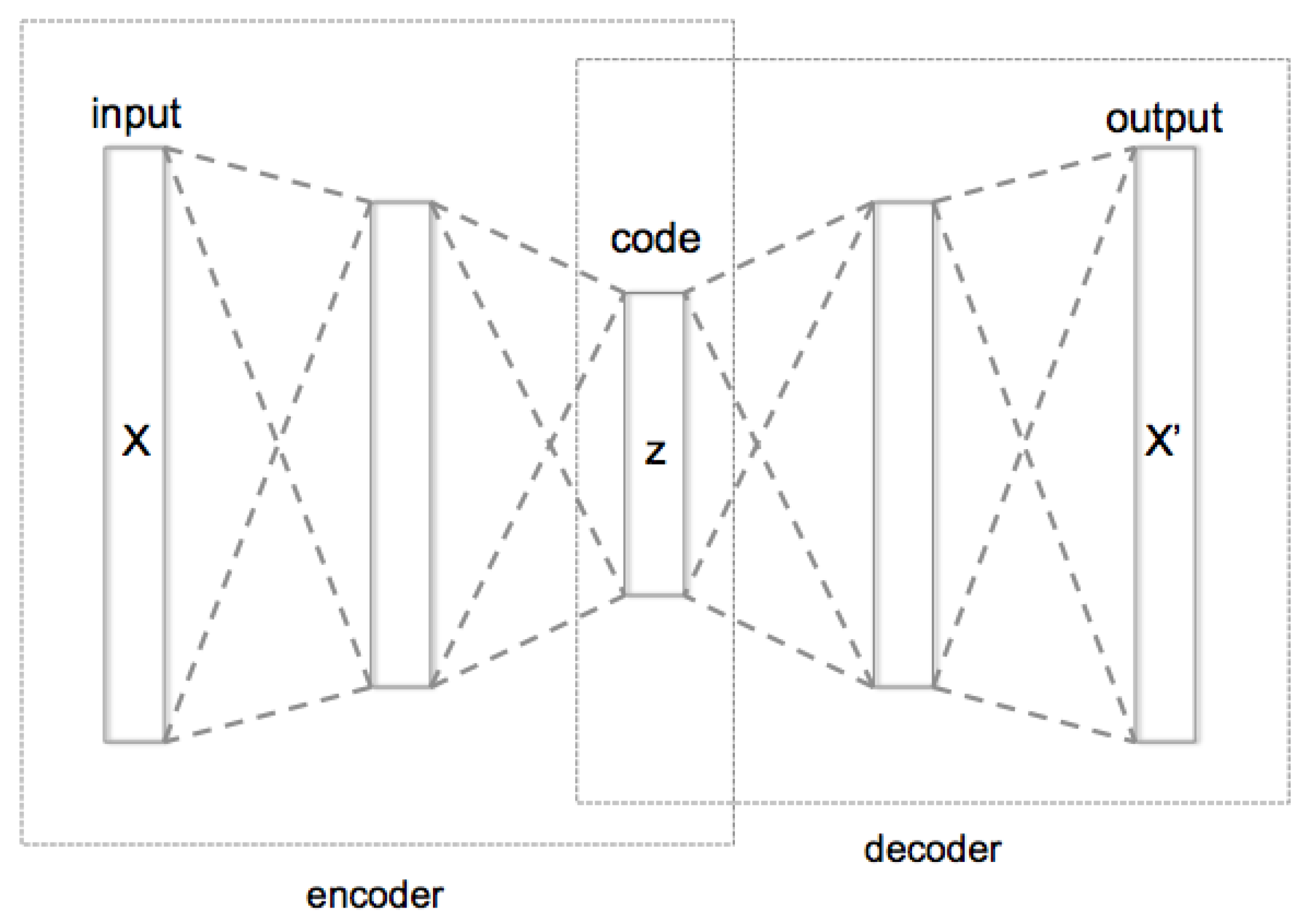
The data point of the reduced dimensionality attack cluster DRDAC has been provided as the input to the AutoEncoder, which is a deep learning-based classifier. This AutoEncoder works well with lesser dimensional data and produces accurate results when data are provided in a clustered manner.
Here, the input is very specific; it is only about the attack packet data and so the AutoEncoder is good in that it classifies based on the attacks. The AutoEncoder will work on the training dataset knowledge, and it will learn through the back propagation from the result of the training data, which is the phase of the decoder and the forward propagation used to find it; it is nothing but a phase of the encoder. The implementation or workflow of the AutoEncoder has been diagrammatically provided in Figure 2.
The AutoEncoder is also capable of doing multiple encode and decode processes on the hidden layers. Equations for the encode and decode processes listed here are in Equations (10) and (11), respectively.
Considering there is a Z dimension vector, the encoder function (e) is defined as in Equation (10).
E i ¯ = e ( D i ¯ , θ e ¯ )
where  D i ¯ R n   a n d   E i   R z .
Similarly, the parameterized function for the decoder (d) is given in Equation (11).
D i ^ = d ( E i ¯ , θ d ¯ )
where  D i ^   R n   a n d   E i   R z .
Whenever the encoded data are taken for the process, the encoded data are reverse propagated to decode it and the actual data are taken for the process. Equation (12) is provided to represent the same.
D i ^ = d ( e ( D i ¯ , θ e ¯ ) , θ d ¯ ) = g ( D i ¯ ,   θ ¯ )
The AutoEncoder back propagates the encoded data with the help of a minimizer with the mean-square-error cost. The function for the same is provided in Equation (13).
C o s t   ( D ,   D ^ , θ ) = 1 m   i ( D ¯ i g ( D i ¯ ,   θ ¯ ) )
The test data are backpropagated with Equation (11) for learning. Finally, the AutoEncoder algorithm will provide the output of the classified attack through the process of Equation (12) by minimizing the mean-square-error cost (MSER) with Equation (13).

7. Dataset and Environment

The environment for execution has been used here as “Python version 3.0”, and the proposed algorithm (PCA + FCM-SMO-AE) is executed in the AWS cloud EC2 instance with the instance family type of t2.micro. The execution has been made in the different environment setups listed in Table 3.
The learning percentage is about the cluster formation module and its learning to classify the data in the attack and non-attack clusters. The test data are about the attack classifier module and the percentage of the total dataset, which is taken as test data for training the AutoEncoder.
The AWS cloud EC2 computing instance setup for executing the proposed algorithm has been given in Table 4.
The dataset we used is CSE-CIC-IDS-2018 [17,19] and it is created based on the network traffic and attack generated on the AWS Cloud in the year 2018. The dataset had 10 .csv files specifying about 10 days of network traffic, with 76 characteristics on each packet and attack carried out across each day, with the date and time of each packet. The details of the attack carried out across dataset have been provided in Table 5.
The considered attacks for this study are the DDoS, DoS, brute-force and botnet attacks, since nearly more than 90% of the attacks on the said dataset fall in the considered four categories.

8. Result and Analysis

The proposed method (PCA + FCM-SMO + AE) has been tested in four different test cases (testing environment conditions) with respect to the learning percentage of the cluster, which is specified in Table 3. The result has been compared with 11 existing techniques, as mentioned here in Table 6.
The existing technique and the proposed technique (PCA + FCM-SMO + AE) have been compared with respect to ten characteristics for evaluation in each of the four test cases. This resulted in 40 comparisons being generated, with 12 statistics in each (11 existing + 1 proposed), totalling 40 × 12 = 480 statistics. The attack taken for the experiments are the DDoS attack, DoS attack, botnet attack and brute-force attack. In each attack category, there will be 480 statistics, resulting in 480 × 4 = 1920 statistics. The average has been taken again to lower the statistics count to 480, since it needs to be discussed here with less complexity. The characteristics are divided into a positive measure, negative measure and other measures.

8.1. Positive Measures

The positive measures taken for the comparison are accuracy, specificity, precision and sensitivity. Equations for each one are given as (14), (15), (16) and (17), respectively.
A c c u r a c y   ( A t t a c k   C l a s s i f i c a t i o n ) = ( T P + T N ) ( T P + T N + F P + F N )
S p e c i f i c i t y   ( A t t a c k   C l a s s i f i c a t i o n ) = T N ( T N + F P )
P r e c i s i o n   ( A t t a c k   C l a s s i f i c a t i o n ) = T P ( T P + F P )
S e n s i t i v i t y   ( A t t a c k   C l a s s i f i c a t i o n ) = T P ( T P + F N )
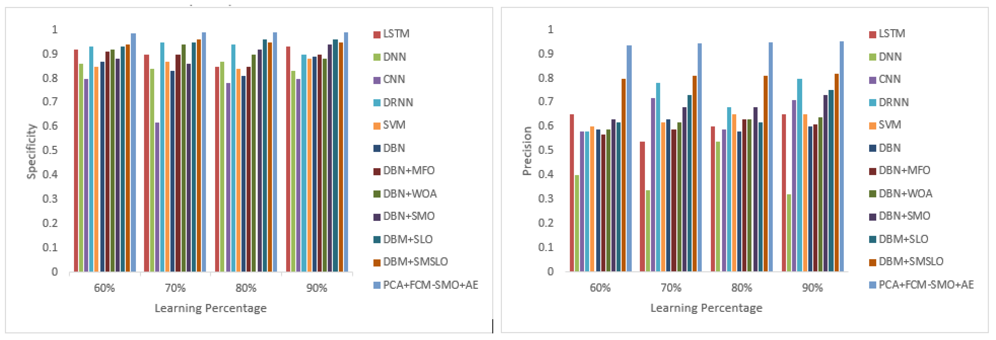
The values obtained in terms of the specificity and precision measures have been given in Figure 3, and the values obtained in terms of sensitivity and accuracy measures has been provided in Figure 4. The proposed technique (PCA + FCM-SMO + AE) has been compared with 11 existing techniques on all metrics with respect to different learning percentages ranging from 60 percent to 90 percent.

8.2. Negative Measures

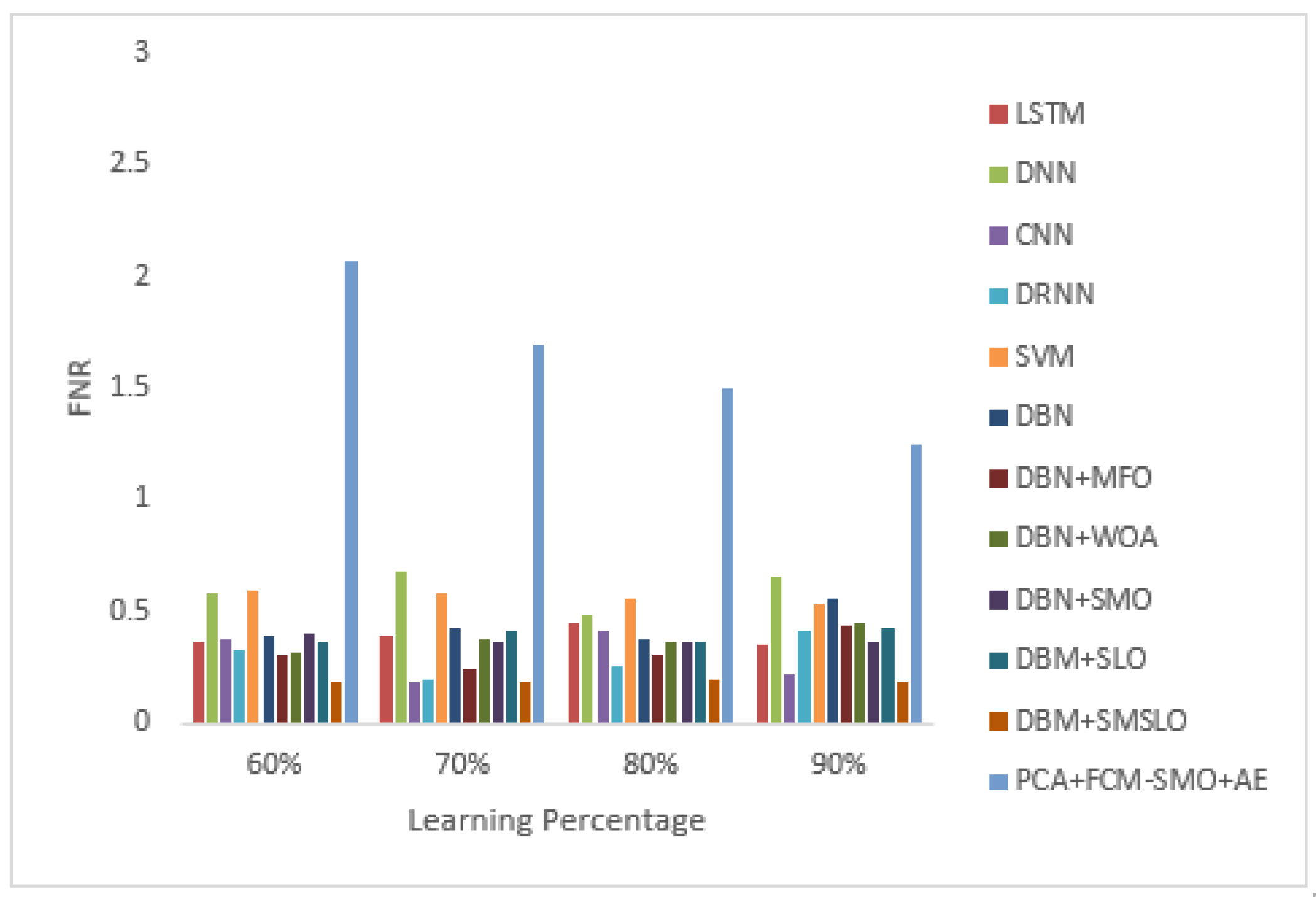
The negative measures taken for the comparison are the false positive rate (FPR), false discovery rate (FDR) and false negative rate (FNR). Equations for each of the measures are provided as (18), (19) and (20), respectively. The values obtained on the comparison basis have been provided on the graph in Figure 5 (FPR and FDR) and Figure 6 (FNR).
F P R   ( A t t a c k   C l a s s i f i c a t i o n ) = F P A c t u a l   N e g a t i v e
F D R   ( A t t a c k   C l a s s i f i c a t i o n ) = F P ( T P + F P )
F N R   ( A t t a c k   C l a s s i f i c a t i o n ) = F N A c t u a l   P o s i t i v e

8.3. Other Measures

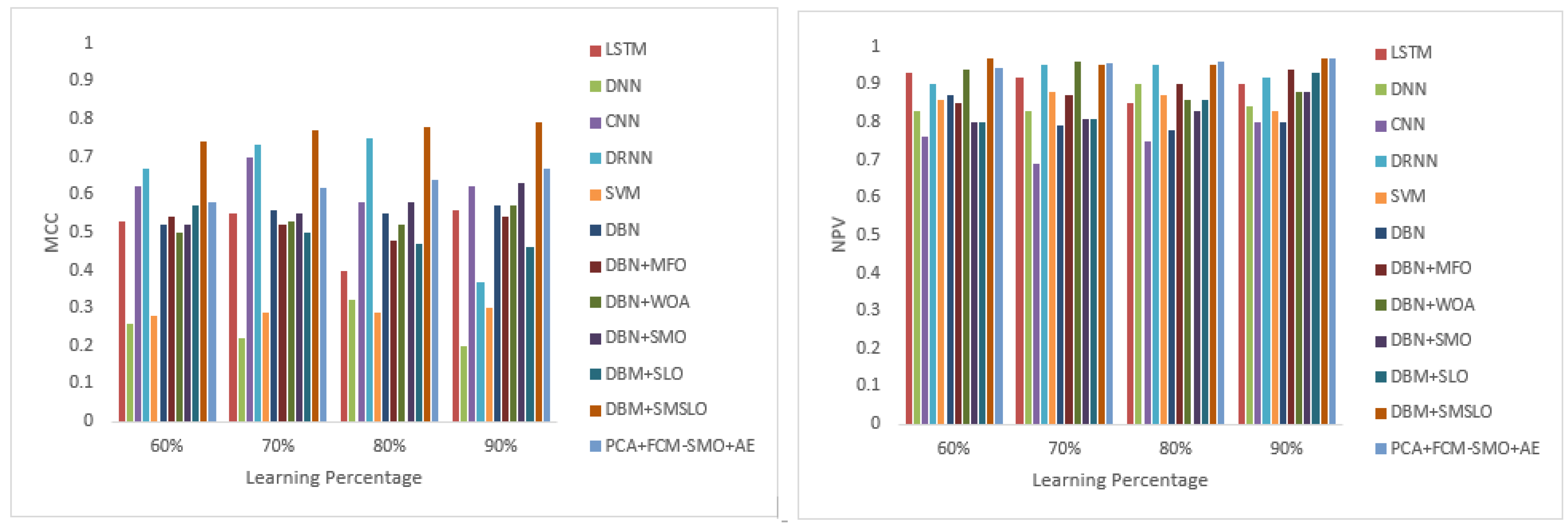
The supportive measures taken for the comparison are the MCC, F-Measure and NPV (Negative Predictive Value). The score of the F-Measure will depend on the precision and sensitivity. When the covariance of these values is higher, then the F-Measure will also be higher. The MCC is nothing but a Matthew’s Correlation Coefficient, which will be less than or equal to one. The max value corresponds to a better prediction of the system. Equations for the MCC, F-Measure and NPV are provided as (21), (22) and (23), respectively.
M C C   ( A t t a c k   C l a s s i f i c a t i o n ) = ( ( T P T N ) ( F P F N ) ) ( ( T P + F P ) ( T N + F P ) ( T P + F N ) ( T N + F N ) ) 2
F M e a s u r e   ( A t t a c k   C l a s s i f i c a t i o n ) = 2 ( p r e c i s i o n s e n s i t i v i t y ) p r e c i s i o n + s e n s i t i v i t y
N P V   ( A t t a c k   C l a s s i f i c a t i o n ) = T N F N + T N
The MCC and NPV values on a comparison basis are shown in Figure 7, and the F-Measure value on a comparison basis has been shown in Figure 8.
The intrusion detected in the AWS cloud network-based dataset for different learning percentage has been provided in Table 7.
The experimental results for the various metrics considered for different learning percentages and the average values are provided in Table 8.
The experimental results of the proposed technique (PCM + FCM-SMO + AE) show that the classified attack with the higher specificity, precision, accuracy and lower FPR and FDR values is a good sign. The MCC, F-Measure and NPV values are comparatively okay. The worst case is the metric values for sensitivity and the FNR. The accuracy of the proposed technique is 95.3%, which is 2.3% higher than the DBN + SMSLO, 12.3% higher than the DBN + SLO, 9.3% higher than the DBN + SMO, 10.3% higher than the DBN + WOA, 15.3% higher than the DBN + MFO, 11.3% higher than the DBN, 18.3% higher than the SVM, 7.3% higher than the DRNN, 35.3% higher than the CNN, 19.3% higher than the DNN and 10.3% higher than the LSTM state-of-the-art existing protocols.

9. Conclusions

The proposed technique takes the data in the CSE-CIC-IDS-2018 dataset. It pre-processed the data and filled the missing values. Then, the dimensionality of the data has been reduced to reduce the complexity, then the dimensionality-reduced data have been provided as inputs to the clustering module, which used the Fuzzy C-Means clustering technique with the Spider Monkey Optimization. The data have been split into attack and non-attack clusters. The attack cluster data values are provided as an input to the attack classifier module, which used the AutoEncoder deep learning-based algorithm to classify the attacks. Finally, the attacks are classified into DDoS, DoS, brute-force and botnet attacks.
The achieved value of the proposed technique (PCM + FCM-SMO + AE) in the positive measures such as specificity (99.0%), precision (94.7%) and accuracy (95.3%) is the highest for the state-of-the-art comparison, but the sensitivity (47.8%) is on the lower side. When the negative measures are considered, the value should be low; the achieved values of proposed techniques against the metrics such as the FPR (0.010) and FDR (0.053) is the lowest in the state-of-the-art comparison, but the FNR (1.627) is on the higher side. The metric measures such as the MCC (0.626), NPV (0.957) and F-Measure (0.635) have been comparatively okay. This makes the conclusion that, overall, the proposed method had beaten the existing 11 state-of-the-art techniques over the CSE-CIC-IDS-2018 dataset, with a 95.3% accuracy in the attack classification prediction.

Author Contributions

B.R.M.—Methodology, validation, formal analysis, investigation, writing—original draft, writing—review and editing, conceptualization. J.K.M.K.—Validation, investigation, writing—review and editing, conceptualization. All authors have read and agreed to the published version of the manuscript.

Funding

This research received no external funding.

Data Availability Statement

Not applicable.

Conflicts of Interest

The authors declare no conflict of interest.

References

  1. Xing, K.; Srinivasan, S.S.R.; Rivera, M.J.; Li, J.; Cheng, X. Attacks and Countermeasures in Sensor Networks: A survey. In Network Security; Springer: Boston, MA, USA, 2010; pp. 251–272. [Google Scholar]
  2. Kumar, C.A.; Vimala, R. Load balancing in cloud environment exploiting hybridization of chicken swarm and enhanced raven roosting optimization algorithm. Multimed. Res. 2020, 3, 45–55. [Google Scholar]
  3. Thomas, R.; Rangachar, M. Hybrid optimization based DBN for face recognition using low-resolution images. Multimed. Res. 2018, 1, 33–43. [Google Scholar]
  4. Veeraiah, N.; Krishna, B. Intrusion detection based on piecewise fuzzy c-means clustering and fuzzy naive bayes rule. Multimed. Res. 2018, 1, 27–32. [Google Scholar]
  5. Preetha, N.N.; Brammya, G.; Ramya, R.; Praveena, S.; Binu, D.; Rajakumar, B. Grey wolf optimisation-based feature selection and classification for facial emotion recognition. IET Biom. 2018, 7, 490–499. [Google Scholar] [CrossRef]
  6. Phan, T.; Park, M. Efficient distributed denial-of-service attack defense in SDN-Based cloud. IEEE Access 2019, 7, 18701–18714. [Google Scholar] [CrossRef]
  7. Ministry of Home Affairs. India Released Facts on Cyber Crime Cases Registered. Available online: https://www.pib.gov.in/PressReleasePage.aspx?PRID=1694783 (accessed on 21 May 2021).
  8. A Study Report Published as a News by University of North Georgia. Available online: https://ung.edu/continuing-education/news-and-media/cybersecurity.php (accessed on 21 May 2021).
  9. 50 Cloud Security Stats You Should Know in 2022. Available online: https://expertinsights.com/insights/50-cloud-security-stats-you-should-know/ (accessed on 28 August 2022).
  10. Amazon Leads $200-Billion Cloud Market. Available online: https://www.statista.com/chart/18819/worldwide-market-share-of-leading-cloud-infrastructure-service-providers/ (accessed on 28 August 2022).
  11. Roy, A.; Razia, S.; Parveen, N.; Rao, A.S.; Nayak, S.R.; Poonia, R.C. Fuzzy rule based intelligent system for user authentication based on user behaviour. J. Discret. Math. Sci. Cryptogr. 2020, 23, 409–417. [Google Scholar] [CrossRef]
  12. Mohan, V.M.; Satyanarayana, K.V.V. The Contemporary Affirmation of Taxonomy and Recent Literature on Workflow Scheduling and Management in Cloud Computing. Glob. J. Comput. Sci. Technol. 2016, 16, 13–21. [Google Scholar]
  13. Zhijun, W.; Wenjing, L.; Liang, L.; Meng, Y. Low-rate DoS attacks, detection, defense, and challenges: A survey. IEEE Access 2020, 8, 43920–43943. [Google Scholar] [CrossRef]
  14. Kumar, R.R.; Shameem, M.; Khanam, R.; Kumar, C. A hybrid evaluation framework for QoS based service selection and ranking in cloud environment. In Proceedings of the 15th IEEE India Council International Conference (INDICON), Coimbatore, India, 16–18 December 2018; IEEE: Piscataway, NJ, USA, 2018; pp. 1–6. [Google Scholar]
  15. Sharma, K.; Ghose, M.K. Wireless Sensor Networks: An Overview on Its Security Threats. IJCA Spec. Issue Mob. Ad-Hoc Netw. MANETs 2010, 1495, 42–45. [Google Scholar]
  16. Mohan, V.M.; Satyanarayana, K. Multi-Objective Optimization of Composing Tasks from Distributed Workflows in Cloud Computing Networks, Advances in Intelligent Systems and Computing Volume 1090. In Proceedings of the 3th International Conference on Computational Intelligence and Informatics ICCII (2018), Hyderabad, India, 28–29 December 2018. [Google Scholar]
  17. Lalitha, V.L.; Raju, D.S.H.; Krishna, S.V.; Mohan, V.M. Customized Smart Object Detection: Statistics of Detected Objects Using IoT; IEEE: Piscataway, NJ, USA, 2021. [Google Scholar]
  18. Kumar, R.R.; Tomar, A.; Shameem, M.; Alam, M.D. Optcloud: An optimal cloud service selection framework using QoS correlation lens. Comput. Intell. Neurosci. 2022, 2022, 2019485. [Google Scholar] [CrossRef]
  19. CSE-CIC-IDS2018 on AWS. Available online: https://www.unb.ca/cic/datasets/ids-2018.html (accessed on 28 August 2022).
  20. IDS 2018 Intrusion CSVs (CSE-CIC-IDS2018). Available online: https://www.kaggle.com/datasets/solarmainframe/ids-intrusion-csv?resource=download (accessed on 28 August 2022).
  21. Somani, G.; Gaur, M.; Sanghi, D.; Conti, M.; Rajarajan, M. Scale inside-out: Rapid mitigation of cloud DDoS attacks. IEEE Trans. Dependable Secur. Comput. 2018, 15, 959–973. [Google Scholar] [CrossRef]
  22. Balajee, R.M.; Mohapatra, H.; Venkatesh, K. A comparative study on efficient cloud security, services, simulators, load balancing, resource scheduling and storage mechanisms. In Proceedings of the IOP Conference Series: Materials Science and Engineering, Tamil Nadu, India, 26–28 March 2021; Volume 1070, p. 012053. [Google Scholar]
  23. Balajee, R.M.; Venkatesh, K. A Survey on Machine Learning Algorithms and finding the best out there for the considered seven Medical Data Sets Scenario. Res. J. Pharm. Technol. 2019, 12, 3059–3062. [Google Scholar] [CrossRef]
  24. Rajeswari, S.; Sharavanan, S.; Vijai, R.; Balajee, R.M. Learning to Rank and Classification of Bug Reports Using SVM and Feature Evaluation. Int. J. Smart Sens. Intell. Syst. 2017, 1, 10. [Google Scholar] [CrossRef] [Green Version]
  25. Ravi, N.; Shalinie, S.M. Learning-driven detection and mitigation of DDoS attack in IoT via SDN-Cloud architecture. IEEE Internet Things J. 2020, 7, 3559–3570. [Google Scholar] [CrossRef]
  26. Virupakshar, K.; Asundi, M.; Narayan, D. Distributed Denial of Service (DDoS) Attacks Detection System for OpenStack-based Private Cloud. Procedia Comput. Sci. 2020, 167, 2297–2307. [Google Scholar] [CrossRef]
  27. Agrawal, N.; Tapaswi, S. Defense mechanisms against DDoS attacks in a cloud computing environment: State-of-the-art and research challenges. IEEE Commun. Surv. Tutor. 2019, 21, 3769–3795. [Google Scholar] [CrossRef]
  28. Khan, A.A.; Shameem, M. Multicriteria decision-making taxonomy for DevOps challenging factors using analytical hierarchy process. J. Softw. Evol. Process. 2020, 32, e2263. [Google Scholar] [CrossRef]
  29. Mohapatra, S.S.; Kumar, R.R.; Alenezi, M.; Zamani, A.T.; Parveen, N. QoS-Aware Cloud Service Recommendation Using Metaheuristic Approach. Electronics 2022, 11, 3469. [Google Scholar] [CrossRef]
  30. Bhardwaj, A.; Mangat, V.; Vig, R. Hyperband tuned deep neural network with well posed stacked sparse autoencoder for detection of DDoS attacks in cloud. IEEE Access 2020, 8, 181916–181929. [Google Scholar] [CrossRef]
  31. Balajee, R.M.; Kannan, M.K.J.; Mohan, V.M. Automatic Content Creation Mechanism and Rearranging Technique to Improve Cloud Storage Space. In Inventive Computation and Information Technologies; Springer: Singapore, 2022; pp. 73–87. [Google Scholar]
  32. Voleti, L.; Balajee, R.M.; Vallepu, S.K.; Bayoju, K.; Srinivas, D. A secure image steganography using improved LSB technique and Vigenere cipher algorithm. In Proceedings of the 2021 International Conference on Artificial Intelligence and Smart Systems (ICAIS), Coimbatore, India, 25–27 March 2021; IEEE: Piscataway, NJ, USA, 2021; pp. 1005–1010. [Google Scholar]
  33. AlKadi, O.; Moustafa, N.; Turnbull, B.; Choo, K. Mixture localization-based outliers models for securing data migration in cloud centers. IEEE Access 2019, 7, 114607–114618. [Google Scholar] [CrossRef]
  34. Devagnanam, J.; Elango, N. Optimal resource allocation of cluster using hybrid grey wolf and cuckoo search algorithm in cloud computing. J. Netw. Commun. Syst. 2020, 3, 31–40. [Google Scholar]
  35. Mishra, P.; Varadharajan, V.; Pilli, E.; Tupakula, U. VMGuard: A VMI-Based Security Architecture for Intrusion Detection in Cloud Environment. IEEE Trans. Cloud Comput. 2020, 8, 957–971. [Google Scholar] [CrossRef]
  36. Dong, S.; Abbas, K.; Jain, R. A survey on distributed denial of service (DDoS) attacks in SDN and cloud computing environments. IEEE Access 2019, 7, 80813–80828. [Google Scholar] [CrossRef]
  37. Thirumalairaj, A.; Jeyakarthic, M. An intelligent feature selection with optimal neural network based network intrusion detection system for cloud environment. Int. J. Eng. Adv. Technol. 2020, 9, 3560–3569. [Google Scholar] [CrossRef]
  38. Roy, R. Rescheduling based congestion management method using hybrid Grey Wolf optimization-grasshopper optimization algorithm in power system. J. Comput. Mech., Power Syst. Control 2019, 2, 9–18. [Google Scholar]
  39. Anand, S. Intrusion detection system for wireless mesh networks via improved whale optimization. J. Netw. Commun. Syst. (JNACS) 2020, 3, 9–16. [Google Scholar] [CrossRef]
  40. Balajee, R.M.; Hiren, K.M.; Rajakumar, B.R. Hybrid machine learning approach based intrusion detection in cloud: A metaheuristic assisted model. Multiagent Grid Syst. 2022, 18, 21–43. [Google Scholar]
  41. Kumar, R.R.; Shameem, M.; Kumar, C. A computational framework for ranking prediction of cloud services under fuzzy environment. Enterp. Inf. Syst. 2021, 16, 167–187. [Google Scholar] [CrossRef]
  42. Tang, T.; McLernon, D.; Mhamdi, L.; Zaidi, S.; Ghogho, M. Intrusion Detection in Sdn-Based Networks: Deep Recurrent Neural Network Approach. In Deep Learning Applications for Cyber Security; Springer: Cham, Switzerland, 2019; pp. 175–195. [Google Scholar]
  43. Bakshi, A.; Dujodwala, Y.B. Securing cloud from ddos attacks using intrusion detection system in virtual machine. In Proceedings of the 2010 Second International Conference on Communication Software and Networks, Singapore, 26–28 February 2010; IEEE: Piscataway, NJ, USA, 2010; pp. 260–264. [Google Scholar]
  44. Fontaine, J.; Kappler, C.; Shahid, A.; De Poorter, E. Log-based intrusion detection for cloud web applications using machine learning. In Proceedings of the International Conference on P2P, Parallel, Grid, Cloud and Internet Computing, Online, 20 October 2019; pp. 197–210. [Google Scholar]
  45. Aboueata, N.; Alrasbi, S.; Erbad, A.; Kassler, A.; Bhamare, D. Supervised machine learning techniques for efficient network intrusion detection. In Proceedings of the 28th International Conference on Computer Communication and Networks (ICCCN), Valencia, Spain, 29 July–1 August 2019; IEEE: Piscataway, NJ, USA, 2019; pp. 1–8. [Google Scholar]
  46. Harikrishna, P.; Amuthan, A. SDN-based DDoS attack mitigation scheme using convolution recursively enhanced self organizing maps. Sādhanā 2020, 45, 1–12. [Google Scholar] [CrossRef]
  47. Bharot, N.; Verma, P.; Sharma, S.; Suraparaju, V. Distributed denial-of-service attack detection and mitigation using feature selection and intensive care request processing unit. Arab. J. Sci. Eng. 2018, 43, 959–967. [Google Scholar] [CrossRef]
  48. Pillutla, H.; Arjunan, A. Fuzzy self organizing maps-based DDoS mitigation mechanism for software defined networking in cloud computing. J. Ambient. Intell. Humaniz. Comput. 2019, 10, 1547–1559. [Google Scholar] [CrossRef]
  49. Bhushan, K.; Gupta, B.B. Network flow analysis for detection and mitigation of Fraudulent Resource Consumption (FRC) attacks in multimedia cloud computing. Multimed. Tools Appl. 2019, 78, 4267–4298. [Google Scholar] [CrossRef]
  50. Baid, U.; Talbar, S. Comparative study of k-means, gaussian mixture model, fuzzy c-means algorithms for brain tumor segmentation. In Proceedings of the International Conference on Communication and Signal Processing 2016 (ICCASP 2016), Online, 26–27 December 2016; pp. 583–588. [Google Scholar]
  51. Khare, N.; Devan, P.; Chowdhary, C.L.; Bhattacharya, S.; Singh, G.; Singh, S.; Yoon, B. Smo-dnn: Spider monkey optimization and deep neural network hybrid classifier model for intrusion detection. Electronics 2020, 9, 692. [Google Scholar] [CrossRef]
  52. Masadeh, R.; Mahafzah, B.A.; Sharieh, A. Sea lion optimization algorithm. Int. J. Adv. Comput. Sci. Appl. 2019, 10. [Google Scholar] [CrossRef] [Green Version]
  53. Kim, J.; Kim, J.; Kim, H.; Shim, M.; Choi, E. CNN-based network intrusion detection against denial-of-service attacks. Electronics 2020, 9, 916. [Google Scholar] [CrossRef]
  54. Sahi, A.; Lai, D.; Li, Y.; Diykh, M. An efficient DDoS TCP flood attack detection and prevention system in a cloud environment. IEEE Access 2017, 5, 6036–6048. [Google Scholar] [CrossRef]
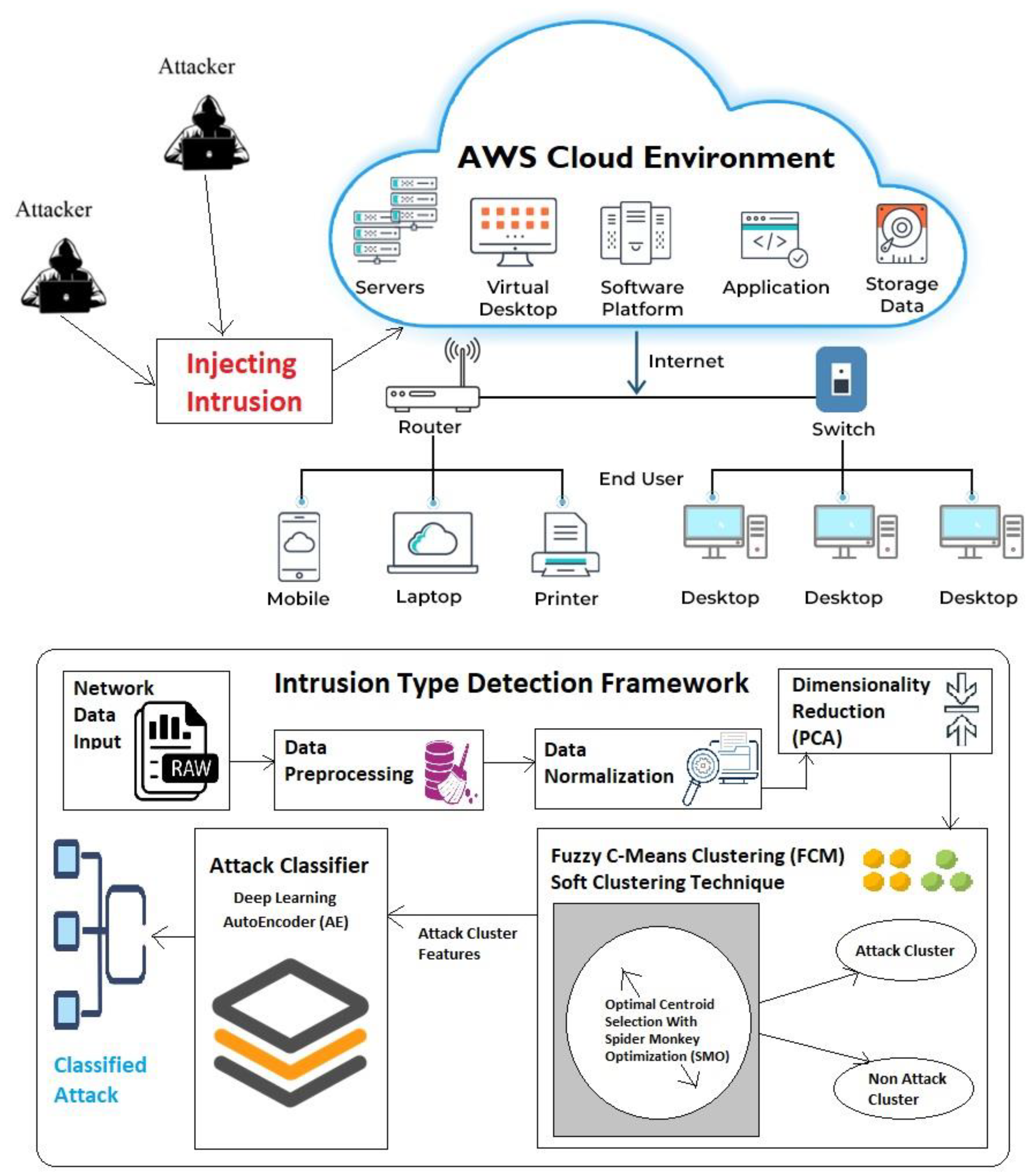
Figure 1. Proposed system (PCA + FCM-SMO + AE) architecture diagram.
Electronics 12 01423 g001
Figure 2. AutoEncoder workflow.
Electronics 12 01423 g002
Figure 3. Specificity and precision comparison graph.
Electronics 12 01423 g003
Figure 4. Sensitivity and accuracy comparison graph.
Electronics 12 01423 g004
Figure 5. FPR and FDR comparision graph.
Electronics 12 01423 g005
Figure 6. FNR comparison graph.
Electronics 12 01423 g006
Figure 7. MCC and NPV comparision graph.
Electronics 12 01423 g007
Figure 8. F-Measure comparison graph.
Electronics 12 01423 g008
Table 2. Nomenclature.
AbbreviationDescription
ANNArtificial Neural Network
CNNConvolution Neural Network
DNNDeep Neural Network
CRESOMConvolution Recursively Enhanced Self-Organizing Map
AEAutoEncoder
CSClassifier System
FCMFuzzy C-Means
DBNDeep Belief Network
SMOSpider Monkey Optimization
DDoSDistributed Denial of Service
DoSDenial of Service
PCAPrincipal Component Analysis
DLDeep learning
DRNNDeep Recurrent Neural Network
DTDecision Trees
SLASea Lion Optimization
FRCFraudulent Resource Consumption
FNRFalse negative rate
FDRFalse discovery rate
FPRFalse positive rate
FSOMDMFuzzy Self-Organizing Maps-based DDOS Mitigation
SVMSupport Vector Machine
GRUGated Recurrent Unit
ICRPUIntensive Care Request Processing Unit
IDSIntrusion Detection System
LEDEMLearning-Driven Detection Mitigation System
LSTMLong Short-Term Memory
MSEMean Square Error
NNNearest Neighbor
RBMRestricted Boltzmann Machine
SDStandard Deviation
SDNMSSoftware Defined Networking-based Mitigation Scheme
FARFloor Area Ratio
Table 3. Learning percentage and testing data.
Learning PercentageTesting Data Considered
60%40%
70%30%
80%20%
90%10%
Table 4. AWS Cloud EC2 computing instance setup.
FeatureDescription
Compute InstanceAWS EC2
Data Storage.csv files in EBS Storage
Instance VPCDefault VPC by AWS
Regionap-south-1
Subnetap-south-1a
Elastic Block Storage Memory8 GB
Instance Architecture64-bit
OSLinux
Security GroupAll Traffic, IPV4 allow anywhere
Client TerminalPutty and putty get for key conversion from.pem to.ppk
FTP Software to transfer datasetFileZila
FTP ConnectionSSH in Port 22
Table 5. Attack details of CSE-CIC-IDS-2018 dataset.
Attacker EnvironmentAttack TypeTools Used for AttackVictim EnvironmentDuration
Kali linuxBruteforce attackFTP—Patator
SSH—Patator
Ubuntu 16.4 (Web Server)One day
Kali linuxDoS attackHulk, GoldenEye,
Slowloris, Slowhttptest
Ubuntu 16.4 (Apache)One day
Kali linuxDoS attackHeartleechUbuntu 12.04 (Open SSL)One day
Kali linuxWeb attackDamn Vulnerable Web App (DVWA)
in-house selenium framework (XSS and brute-force)
Ubuntu 16.4 (Web Server)Two days
Kali linuxInfiltration attackFirst level: dropbox download in a Windows machine.
Second level: Nmap and portscan
Windows Vista and MacintoshTwo days
Kali linuxBotnet attackAres (developed by Python): remote shell, file upload/download, capturing
screenshots and key logging
Windows Vista, 7, 8.1, 10 (32-bit) and 10 (64-bit)One day
Kali linuxDDoS + PortScanLow Orbit Ion Canon (LOIC) for UDP, TCP or HTTP requestsWindows Vista, 7, 8.1, 10 (32-bit) and 10 (64-bit)Two days
Table 6. Existing best technique for intrusion detection of CSE-CIC-IDS-2018 dataset.
Technique ShortformReference Paper NumberTechnique Full Name
SVM classifier[2]Support Vector Machine
LSTM[42]Long-Short Term Memory
DNN[6]Deep Neural Network
DRNN[43]Deep Recurrent Neural Network
CNN[41]Convolution Neural Network
DBN[1]Deep Belief Network
DBN + WOA[1]Deep Belief Network with Whale Optimization Algorithm
DBN + MFO[1]Deep Belief Network with Moth Flame Optimization
DBN + SLO[1]Deep Belief Network with Sea Lion Optimization
DBN + SMO[1]Deep Belief Network with Spider Monkey Optimization
DBN + SMSLO[1]Deep Belief Network with Spider Monkey optimization and Sea Lion Optimization
Table 7. Intrusion detection details with respect to learning percentage.
DDOS AttackDOS AttackBrute-Force AttackBotnet Attack
Learning Percentage: 60% and Test Data: 40%
Predicted Positive3,464,454414,564219,911164,846
Predicted Negative7,356,52410,406,41310,601,06710,656,132
TP3,115,042370,988216,017160,210
TN7,110,7829,729,6959,956,39010,031,606
FP349,41243,57638944636
FN245,742676,718644,677624,526
Learning Percentage: 70% and Test Data: 30%
Predicted Positive4,003,406480,911257,899191,118
Predicted Negative8,621,06812,143,56412,366,57512433,356
TP3,691,901435,110250,951188,314
TN8,410,03611,472,97611,739,36011,852,630
FP311,50445,80169492805
FN211,032670,588627,215580,726
Learning Percentage: 80% and Test Data: 20%
Predicted Positive4,570,926547,518295,964219,795
Predicted Negative9,857,04513,880,45214,132,00714,208,176
TP4,236,896500,409287,717215,674
TN9,631,53613,209,30413,472,90213,631,057
FP334,02947,11082474121
FN225,509671,148659,105577,119
Learning Percentage: 90% and Test Data: 10%
Predicted Positive5,127,458612,425329,867245,981
Predicted Negative11,104,00915,619,04215,901,60015,985,486
TP4,776,398564,726322,994242,118
TN10,891,91215,016,89315,204,67815,494,678
FP351,06047,69868723864
FN212,097602,149696,922490,808
Table 8. Experimental results for considered metrics.
MeasureLSTMDNNCNNDRNNSVMDBNDBN + MFODBN + WOADBN + SMODBM + SLODBM + SMSLOPCA + FCM-SMO + AE
Learning Percentage: 60% and Test Data: 40%
Specificity0.9200.8600.8000.9300.8500.8700.9100.9200.8800.9300.9400.987
Precision0.6500.4000.5800.5800.6000.5900.5700.5900.6300.6200.8000.937
Sensitivity0.6600.4200.5000.5900.3600.6200.6100.6200.6200.6600.8100.434
Accuracy0.8700.7300.6600.8800.7800.8500.8200.8500.8400.8500.9100.940
MCC0.5300.2600.6200.6700.2800.5200.5400.5000.5200.5700.7400.581
F-Measure0.6550.4100.5370.5850.4500.6050.5890.6050.6250.6390.8050.593
NPV0.9300.8300.7600.9000.8600.8700.8500.9400.8000.8000.9700.946
FPR0.0900.1300.5000.0800.1500.1100.0900.1100.0800.0900.0600.013
FDR0.3800.5900.4100.3500.5600.3900.3400.4100.3600.4200.1800.063
FNR0.3700.5800.3800.3300.6000.3900.3000.3200.4000.3600.1802.062
Learning Percentage: 70% and Test Data: 30%
Specificity0.9000.8400.6200.9500.8700.8300.9000.9400.8600.9500.9600.990
Precision0.5400.3400.7200.7800.6200.6300.5900.6200.6800.7300.8100.946
Sensitivity0.6600.3600.7600.7500.4200.6200.5800.6200.6100.6600.8300.468
Accuracy0.8500.8000.5200.9200.7400.8200.7800.8500.8500.8400.9300.951
MCC0.5500.2200.7000.7300.2900.5600.5200.5300.5500.5000.7700.618
F-Measure0.5940.3500.7390.7650.5010.6250.5850.6200.6430.6930.8200.626
NPV0.9200.8300.6900.9500.8800.7900.8700.9600.8100.8100.9500.956
FPR0.0800.1700.7500.0700.1300.0800.1100.0900.0600.0700.0500.010
FDR0.3800.6800.1700.2000.5700.3300.2200.7000.3600.4700.1900.054
FNR0.3900.6800.1800.2000.5800.4300.2400.3800.3600.4100.1901.691
Learning Percentage: 80% and Test Data: 20%
Specificity0.8500.8700.7800.9400.8400.8100.8500.9000.9200.9600.9500.991
Precision0.6000.5400.5900.6800.6500.5800.6300.6300.6800.6200.8100.949
Sensitivity0.5200.4800.5000.7000.4400.6100.5900.6100.6300.6300.8000.488
Accuracy0.8300.7900.5900.9000.7700.8300.8000.8400.8500.7900.9200.956
MCC0.4000.3200.5800.7500.2900.5500.4800.5200.5800.4700.7800.638
F-Measure0.5570.5080.5410.6900.5250.5950.6090.6200.6540.6250.8050.645
NPV0.8500.9000.7500.9500.8700.7800.9000.8600.8300.8600.9500.960
FPR0.1500.1300.6300.0500.1400.0800.0800.0900.0700.0800.0500.009
FDR0.4600.4800.4100.2500.5700.3100.3400.4100.4200.3800.2000.051
FNR0.4500.4900.4200.2600.5600.3800.3000.3700.3600.3600.2001.503
Learning Percentage: 90% and Test Data: 10%
Specificity0.9300.8300.8000.9000.8800.8900.9000.8800.9400.9600.9500.991
Precision0.6500.3200.7100.8000.6500.6000.6100.6400.7300.7500.8200.954
Sensitivity0.6000.3400.6400.8000.5000.6300.6200.6300.6600.6500.8000.522
Accuracy0.8500.7200.6300.8200.7900.8600.8000.8600.9000.8400.9600.963
MCC0.5600.2000.6200.3700.3000.5700.5400.5700.6300.4600.7900.669
F-Measure0.6240.3300.6730.8000.5650.6150.6150.6350.6930.6960.8100.675
NPV0.9000.8400.8000.9200.8300.8000.9400.8800.8800.9300.9700.967
FPR0.0900.1800.6400.0900.1400.0900.1200.0800.0700.0800.0400.009
FDR0.3400.6500.2100.4000.5800.4100.3800.6400.3800.4900.1900.046
FNR0.3500.6500.2200.4100.5400.5600.4400.4500.3600.4300.1901.250
Average Value Results
Specificity0.9000.8500.7500.9300.8600.8500.8900.9100.9000.9500.9500.990
Precision0.6100.4000.6500.7100.6300.6000.6000.6200.6800.6800.8100.947
Sensitivity0.6100.4000.6000.7100.4300.6200.6000.6200.6300.6500.8100.478
Accuracy0.8500.7600.6000.8800.7700.8400.8000.8500.8600.8300.9300.953
MCC0.5100.2500.6300.6300.2900.5500.5200.5300.5700.5000.7700.626
F-Measure0.6080.3990.6230.7100.5100.6100.6000.6200.6540.6640.8100.635
NPV0.9000.8500.7500.9300.8600.8100.8900.9100.8300.8500.9600.957
FPR0.1030.1530.6300.0730.1400.0900.1000.0930.0700.0800.0500.010
FDR0.3900.6000.3000.3000.5700.3600.3200.5400.3800.4400.1900.053
FNR0.3900.6000.3000.3000.5700.4400.3200.3800.3700.3900.1901.627
Disclaimer/Publisher’s Note: The statements, opinions and data contained in all publications are solely those of the individual author(s) and contributor(s) and not of MDPI and/or the editor(s). MDPI and/or the editor(s) disclaim responsibility for any injury to people or property resulting from any ideas, methods, instructions or products referred to in the content.