Distributed Stochastic Model Predictive Control for a Microscopic Interactive Traffic Model

Abstract

Stochastic Model Predictive Control (SMPC) has attracted increasing attention for autonomous driving in recent years, since it enables collision-free maneuvers and trajectory planning and can deal with uncertainties in a non-conservative way. Many promising strategies have been proposed on how to use SMPC to select appropriate maneuvers and plan safe trajectories in uncertain environments. The limitation of these approaches is that they focus on scenarios where only one vehicle is controlled by SMPC and is, thus, reacting to the surrounding vehicles; however, the surrounding vehicles do not react to the SMPC-controlled vehicle, which means there is no mutual interaction. However, when multiple autonomous vehicles are driving on the road, each individual vehicle will take the behavior of the other surrounding vehicles into account and adjust its individual decisions accordingly in trajectory planning. This paper, therefore, examines in simulations how the interactive control system of multiple SMPC-controlled vehicles behave based on a Distributed SMPC (DSMPC) framework. For a three-lane highway scenario, we first investigate the effects of the risk parameter of the collision avoidance probabilistic constraint on non-interactive and interactive vehicle systems and provide insights into how to parameterize the controllers in interactive vehicle systems.

1. Introduction

Recent decades have witnessed rapid development in autonomous driving. Autonomous vehicles driving in dynamic highway environments must be able to manage the uncertainty resulting from the behavior of other traffic participants [1]. Nominal control approaches that cannot deal with system uncertainties might cause hazardous performance [1]. In contrast, robust control approaches can consider uncertainties but are too conservative because they also consider worst-case scenarios [2]. SMPC has been used to control autonomous vehicles because of its ability to consider uncertainties and simultaneously avoid overly conservative behaviors [1,3,4,5].

MPC iteratively solves a constrained optimal-control problem on a finite prediction horizon. That means a cost function is minimized while satisfying multiple constraints [6], including a system dynamic model used for generating predictions and safety constraints. In contrast, SMPC allows constraint violation with a specified small probability by applying probabilistic chance constraints, resulting in non-conservative behaviors [7,8]. Autonomous vehicles controlled by SMPC treat collision-avoidance constraints with adjustable risk parameters as probabilistic constraints [1,4]. However, in previous studies [1,3,4,5], simulations that confirmed the suitability of SMPC-based controllers for autonomous vehicles assumed that the surrounding vehicles used a much simpler controller and, in particular, did not consider predictions of the surrounding vehicles and, thus, also did not react to SMPC-controlled vehicles.

In the simulations of this paper, for simplicity of description, vehicles that react to other vehicles are called reactive vehicles, and those that do not react to other vehicles are non-reactive vehicles. A system consisting of only one reactive vehicle and multiple non-reactive vehicles is a non-interactive system. In real traffic, all vehicles tend to react to the vehicles in the environment. Thus, after designing an individual SMPC algorithm for a vehicle treating all surrounding vehicles as non-reactive vehicles, it is essential to also embed this controlled vehicle system in an environment where all surrounding vehicles are reactive. We, thus, obtain an interactive system. Not only is it important to investigate the performance of the overall interactive control system but the findings from this investigation must be included in the design of the SMPC for an individual autonomous vehicle.

Evaluating the performance of a novel controller requires simulating it in different scenarios employing either microscopic traffic models or macroscopic traffic models. Microscopic traffic models focus on studying the traffic phenomena of individual vehicles and analyzing how they interact with each other [9]. In microscopic traffic models, the dynamics of each traffic participant are individually modeled [10]; this allows us to know each vehicle’s detailed information, including the location, velocity, inertial heading, acceleration, and steering angle [10]. Macroscopic traffic models research the overall characteristics, e.g., the intensity, density, and mean speed, of the traffic flow, in which the details of individual interactions between vehicles are ignored [9,11]. In this paper, we study the performance of individual SMPC-controlled vehicles and the interactions between them and, consequently, select a microscopic traffic model.

In a multi-vehicle highway environment, considering the interactions between reactive vehicles contributes to more precise traffic prediction [12], which is fundamentally required in intelligent transportation systems [11]. Interactions between reactive vehicles have previously been investigated in microscopic traffic simulations [12,13]; however, to the best of our knowledge, the interactions between SMPC-controlled vehicles, where it is of interest to see the impact and the interplay of different risk parameters that determine the aggressiveness/conservativeness level of vehicles when reacting to other vehicles, have not been investigated. This motivated us to examine the interactions between SMPC-controlled vehicles in a multi-vehicle interactive system for a highway environment in this paper.

To do this, we model the multi-vehicle interactive system using a Distributed SMPC (DSMPC) framework [14,15,16]. In this framework, each vehicle interacts with its surrounding vehicles by observing their current states and predicting their future behaviors and avoiding potential collisions. Distributed MPC (DMPC) has been applied to solve vehicle platooning problems [17,18,19,20], where multiple vehicles are typically involved and are controlled to cruise at a constant speed. However, DMPC has not been used for problems where individual vehicles do not have a common driving goal. In this paper, we use a DSMPC framework to model multi-vehicle interactive systems, where individual vehicles have unique driving goals, which are usually different. Here, we assume that all vehicles have the same controller but with different parameterizations. In particular, the risk parameter is chosen differently.

We summarize the contributions of this paper as follows:

• Investigating the effects of SMPC risk parameters on non-interactive and interactive vehicle-control systems on highways.
• Providing guidelines on how to set risk parameters for vehicles in interactive systems.

Our work regarding interactive systems of SMPC-controlled vehicles is based on the hypotheses below:

Hypothesis 1.

The behaviors of a vehicle are determined not only by its own controller but also by the controllers of other vehicles.

Hypothesis 2.

The behaviors of one vehicle can influence the performance of the whole system.

The rest of the paper is organized as follows. Section 2 presents the communication topology used in the distributed framework and formulates the individual SMPC controller and how all individual SMPC controllers are combined together. In Section 3, we introduce elements of these SMPC problems and transform the stochastic optimal-control problem into a deterministic problem. Finally, our simulation results are presented in Section 4 followed by our conclusions in Section 5.

Notation: $\mathbb{R}$ is the set of real numbers. ${\mathbb{R}}^m$ denotes the set of all column vectors with m elements, which are real numbers. ${\mathbb{R}}^{m\times n}$ stands for the set of all $m\times n$ matrices whose elements are real numbers. We use ${\mathbb{S}}^n$ to denote the set of symmetric matrices of order n. ${\parallel \mathit{x}\parallel }_Q^2={\mathit{x}}^{⊺}Q\mathit{x}$.

2. Model of the Multi-Vehicle System

In our multi-vehicle interactive control system model, each vehicle detects the position in the lateral and longitudinal direction, velocity, and inertial heading angle of all currently neighboring vehicles, which we refer to as ’information’ in the following; a graph theoretic time-varying communication topology [19] models this information transmission.

In this section, we introduce the communication topology and the SMPC problem that is solved by an individual vehicle and how all SMPC problems are combined into the distributed SMPC control framework.

2.1. Communication Topology

The communication topology shows which of the surrounding vehicles is considered in the controller of one particular vehicle. We assume that all vehicles are equipped with sensors to detect information about their surrounding vehicles at a specified detectable distance. This distance depends on the detection ability of each vehicle’s sensors. For simplicity, we assume that the sensors of all vehicles have the same detection ability, which means the detectable distance is the same.

Here, we introduce a communication topology at one time step as shown in Figure 1. The communication topology is updated at each time step to account for changing vehicle positions.

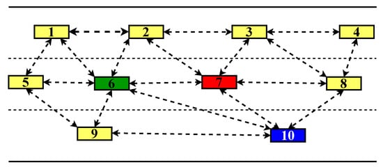
Figure 1. Communication topology at one time step. This topology shows, at one time step, which of the surrounding vehicles is considered in the controller of one particular vehicle. This topology is updated at each time step.

It is modeled as an undirected graph $\mathbb{G}=\{\mathbb{V},\mathbb{E}\}$, where $\mathbb{V}=\{1,2,\dots ,N_v\}$ is the set of nodes, which represent vehicles, and  $\mathbb{E}\subseteq \mathbb{V}\times \mathbb{V}$ is the set of edges describing the information detection among vehicles. The number of nodes (vehicles) in the graph is given by $N_v$. The graph $\mathbb{G}$ can be denoted with an adjacency matrix $\mathcal{A}\in {\mathbb{R}}^{N_v\times N_v}$

$$\mathcal{A}=\left[a_{ij}\right]=\left\{\begin{array}{cc}\hfill a_{ij}& =1,\mathrm{if}\{i,j\}\in \mathbb{E}\hfill \\ \hfill a_{ij}& =0,\mathrm{if}\{i,j\}\notin \mathbb{E}\hfill \end{array}\right.,$$

(1)

where $\{i,j\}\in \mathbb{E}$ means vehicle i senses the information about vehicle j, which is within the detectable distance of vehicle i. Vehicle j is, therefore, a neighbor of vehicle i. The set consisting of the neighbors of vehicle i is denoted by ${\mathbb{N}}_i=\{j\mid a_{ij}=1,j\in \mathbb{V}\}$. We define a dual set ${\mathbb{O}}_i=\{j\mid a_{ji}=1,j\in \mathbb{V}\}$, which includes all vehicles that identify i as a neighbor. The union of the two sets ${\mathbb{N}}_i$ and ${\mathbb{O}}_i$ is ${\mathbb{N}}_i\cup {\mathbb{O}}_i$. All vehicles in ${\mathbb{N}}_i\cup {\mathbb{O}}_i$ categorize i as one of their neighbors and are themselves simultaneously neighbors of vehicle i. The sets ${\mathbb{N}}_i$, ${\mathbb{O}}_i$, and ${\mathbb{N}}_i\cup {\mathbb{O}}_i$ are updated at each sampling time. Assuming that all vehicles have the same detectable distance, the sets ${\mathbb{N}}_i$, ${\mathbb{O}}_i$, and ${\mathbb{N}}_i\cup {\mathbb{O}}_i$ are equal.

Each controlled vehicle will attempt to avoid collisions with its neighboring vehicles, and probabilistic constraints in the optimal-control problem reflect this requirement. Any vehicle i incorporates the information about its neighbors from ${\mathbb{N}}_i$ into its collision-avoidance constraints. All vehicles in ${\mathbb{O}}_i$ take the information of vehicle i into account in their collision-avoidance constraints.

2.2. Vehicle Controllers

The multi-vehicle interactive control system consists of a number of individual vehicles that are interactive because their individual controllers consider information about the current states of surrounding vehicles. We assume that each vehicle is controlled by SMPC; thus, the overall system is modeled using a distributed SMPC framework. The SMPC optimal-control problem that is solved by each vehicle at every sampling time is introduced in this section.

To decide on the current optimal control, each controlled vehicle, denoted as an Ego Vehicle (EV), must consider its predicted behaviors as well as those of vehicles, denoted as Target Vehicles (TVs), within a detectable distance. Simultaneously, an EV might be a TV of other Ego Vehicles (EVs). For each vehicle i ($i\in \mathbb{V}$) and each prediction time step k $(k=0,\dots ,N-1)$, we define the predicted state ${\mathit{\xi }}_{i,k}^{\mathrm{p}}$ and predicted control input ${\mathit{u}}_{i,k}^{\mathrm{p}}$ that will later be optimized over a prediction horizon of length N. Further, we introduce assumed states ${\mathit{\xi }}_{i,k}^{\mathrm{a}}$ and assumed control inputs ${\mathit{u}}_{i,k}^{\mathrm{a}}$ [18,19] to describe what other vehicles (vehicles in ${\mathbb{O}}_i$) assume about the future behaviors of vehicle i. Finally, ${\mathit{\xi }}_{i,k}^{*}$ and ${\mathit{u}}_{i,k}^{*}$ define the optimal trajectories that vehicle i determines by solving the SMPC optimal control problem.

The SMPC optimal-control problem for EV $i\in \mathbb{V}$ is specified by a cost function $J_i$ and constraints. The cost function is minimized over all admissible control input trajectories ${\mathit{u}}_i^{\mathrm{p}}={\left({\mathit{u}}_{i,0}^{\mathrm{p}},{\mathit{u}}_{i,1}^{\mathrm{p}},\dots ,{\mathit{u}}_{i,N-1}^{\mathrm{p}}\right)}^{⊺}$, where admissibility means that the control inputs ${\mathit{u}}_i^{\mathrm{p}}$ as well as the corresponding state trajectory ${\mathit{\xi }}_i^{\mathrm{p}}={\left({\mathit{\xi }}_{i,0}^{\mathrm{p}},{\mathit{\xi }}_{i,1}^{\mathrm{p}},\dots ,{\mathit{\xi }}_{i,N}^{\mathrm{p}}\right)}^{⊺}$, which is found by iterating the system dynamics

$${\mathit{\xi }}_{i,k+1}^{\mathrm{p}}={\mathit{f}}^{\mathrm{p}}\left({\mathit{\xi }}_{i,k}^{\mathrm{p}},{\mathit{u}}_{i,k}^{\mathrm{p}}\right),i\in \mathbb{V},k=0,\dots ,N-1,$$

(2a)

do not violate constraints. The initial predicted state ${\mathit{\xi }}_{i,0}^{\mathrm{p}}$ is the current state of the EV i. A first version of the optimal-control problem is, thus, given by

$$\underset{{\mathit{u}}_i^{\mathrm{p}}}{min}{\mathit{J}}_i\left({\mathit{\xi }}_i^{\mathrm{p}},{\mathit{u}}_i^{\mathrm{p}}\right)$$

(2b)

subject to state and input constraints

$${\mathit{\xi }}_i^{\min }\le {\mathit{\xi }}_{i,k}^{\mathrm{p}}\le {\mathit{\xi }}_i^{\max },k=0,\dots ,N$$

(2c)

$${\mathit{u}}_i^{\min }\le {\mathit{u}}_{i,k}^{\mathrm{p}}\le {\mathit{u}}_i^{\max },k=0,\dots ,N-1.$$

(2d)

Remark: We used only box constraints here, though more general constraints would be allowed.

We still have to add collision-avoidance constraints that involve assumptions on the surrounding vehicles’ behaviors. Summarizing the assumed models of all TVs in

$${\mathit{\xi }}_{\mathrm{TV},k+1}^{\mathrm{a}}={\mathit{f}}_{\mathrm{TV}}^{\mathrm{a}}\left({\mathit{\xi }}_{\mathrm{TV},k}^{\mathrm{a}},{\mathit{u}}_{\mathrm{TV},k}^{\mathrm{a}},{\mathit{\omega }}_{\mathrm{TV},k}^{\mathrm{a}}\right),k=0,\dots ,N-1,$$

(2e)

where ${\mathit{\omega }}_{\mathrm{TV},k}^{\mathrm{a}}$ is the uncertainty in the prediction of TV behaviors, we obtain assumptions for all times in the prediction horizon used to formulate probabilistic collision-avoidance constraints for each TV summed up in

$$\mathrm{Pr}\left({\mathit{\xi }}_{i,k}^{\mathrm{p}}\in {\Xi }_{i,k}^{\mathrm{safe},\mathrm{TV}}\right)\ge p_i,p_i\in [0.5,1],k=1,\dots ,N.$$

(2f)

These constraints are probabilistic constraints in our approach. The requirement ${\mathit{\xi }}_{i,k}^{\mathrm{p}}\in {\Xi }_{i,k}^{\mathrm{safe},\mathrm{TV}}$ means that states ${\mathit{\xi }}_{i,k}^{\mathrm{p}}$ have to be in the safe set ${\Xi }_{i,k}^{\mathrm{safe},\mathrm{TV}}$ to avoid potential collisions with the TVs at prediction step k. The set ${\Xi }_{i,k}^{\mathrm{safe},\mathrm{TV}}$ is determined from the predicted states of EV i and the assumed states of all its TVs ${\mathit{\xi }}_{\mathrm{TV},k}^{\mathrm{a}}$. Employing $\mathrm{Pr}\left(*\right)\ge p_i$, we ensure that the event ∗ occurs with a probability of not less than $p_i$. The probabilistic constraints (2f) are designed to soften the collision-avoidance constraint between the EV i and its TVs.

A small probability of collisions between the EV i and its TVs is acceptable. This softening prevents overly conservative driving behaviors caused by hard constraints in robust MPC. In the following, $p_i$ in constraints (2f) is identified as a risk parameter of EV i and is specified in advance. A smaller risk parameter $p_i$ corresponds to more aggressive driving behaviors, which might increase the probability of collisions. Conversely, a larger $p_i$ results in more conservative behaviors, a defensive driving mode.

We refer to the expressions (2a)–(2f) as ’the SMPC optimal-control problem’ in the following. The model in (2e) collects the system models of all TVs of EV i. If we assume that EV i takes m TVs labeled $i_1,i_2,\dots ,i_m$ ($i_1,i_2,\dots ,i_m\in {\mathbb{N}}_i$) into account, then (2e) summarizes

$$\left\{\begin{array}{c}{\mathit{\xi }}_{i_1,k+1}^{\mathrm{a}}={\mathit{f}}^{\mathrm{a}}\left({\mathit{\xi }}_{i_1,k}^{\mathrm{a}},{\mathit{u}}_{i_1,k}^{\mathrm{a}},{\mathit{\omega }}_{i_1,k}^{\mathrm{a}}\right)\hfill \\ {\mathit{\xi }}_{i_2,k+1}^{\mathrm{a}}={\mathit{f}}^{\mathrm{a}}\left({\mathit{\xi }}_{i_2,k}^{\mathrm{a}},{\mathit{u}}_{i_2,k}^{\mathrm{a}},{\mathit{\omega }}_{i_2,k}^{\mathrm{a}}\right)\hfill \\ ⋮\hfill \\ {\mathit{\xi }}_{i_m,k+1}^{\mathrm{a}}={\mathit{f}}^{\mathrm{a}}\left({\mathit{\xi }}_{i_m,k}^{\mathrm{a}},{\mathit{u}}_{i_m,k}^{\mathrm{a}},{\mathit{\omega }}_{i_m,k}^{\mathrm{a}}\right)\hfill \end{array}\right.,k=0,\dots ,N-1.$$

(3)

The assumed states ${\mathit{\xi }}_{i_1,k}^{\mathrm{a}}$, ${\mathit{\xi }}_{i_2,k}^{\mathrm{a}}$, and ${\mathit{\xi }}_{i_m,k}^{\mathrm{a}}$ correspond to TVs $i_1$, $i_2$, and $i_m$, respectively. Similarly, the assumed control inputs are ${\mathit{u}}_{i_1,k}^{\mathrm{a}}$, ${\mathit{u}}_{i_2,k}^{\mathrm{a}}$, and ${\mathit{u}}_{i_m,k}^{\mathrm{a}}$; the prediction uncertainties are denoted by ${\mathit{\omega }}_{i_1,k}^{\mathrm{a}}$, ${\mathit{\omega }}_{i_2,k}^{\mathrm{a}}$, and ${\mathit{\omega }}_{i_m,k}^{\mathrm{a}}$. The dynamic model of the EV and TVs will be discussed in more detail in Section 3.

In the same way, expression (2f) contains the collision-avoidance constraints between EV i and all its TVs ($i_1,i_2,\dots ,i_m\in {\mathbb{N}}_i$):

$$\left\{\begin{array}{c}\mathrm{Pr}\left({\mathit{\xi }}_{i,k}^{\mathrm{p}}\in {\Xi }_{i,k}^{\mathrm{safe},i_1}\right)\ge p_i\hfill \\ \mathrm{Pr}\left({\mathit{\xi }}_{i,k}^{\mathrm{p}}\in {\Xi }_{i,k}^{\mathrm{safe},i_2}\right)\ge p_i\hfill \\ ⋮\hfill \\ \mathrm{Pr}\left({\mathit{\xi }}_{i,k}^{\mathrm{p}}\in {\Xi }_{i,k}^{\mathrm{safe},i_m}\right)\ge p_i\hfill \end{array}\right.,p_i\in [0.5,1],k=1,\dots ,N.$$

(4)

Here, ${\Xi }_{i,k}^{\mathrm{safe},i_1}$, ${\Xi }_{i,k}^{\mathrm{safe},i_2}$ and ${\Xi }_{i,k}^{\mathrm{safe},i_m}$ are the sets of safe states of EV i for preventing collisions with TVs $i_1$, $i_2$, ⋯, $i_m$ at prediction step k, respectively.

3. Elements of the SMPC Problem

In this section, we introduce the elements of the SMPC optimal-control problem, including the vehicle models in Section 3.1, constraints in Section 3.2, and cost function in Section 3.3.

Additionally, due to the presence of stochastic disturbances ${\mathit{\omega }}_{\mathrm{TV},k}^{\mathrm{a}}$ in the TV model (2e) and the probabilistic chance constraints (2f), the SMPC optimal-control problem cannot be solved directly [1]. To solve this, we transfer the stochastic optimal-control problem into a deterministic one by (1) reformulating the dynamic model of the TV, as shown in Section 3.1.4; and (2) tightening the probabilistic constraints as shown in Section 3.2.3.

3.1. Vehicle Models

A predictive controller requires a system model (2a). Thus, for our application, we need a system model of each EV, which is used by the EV to decide on optimal controls. In addition, we need a system model of each TV, which EVs use to predict TV trajectories to avoid potential collisions.

Vehicle models with different modeling depths have been proposed in the literature, including, e.g., the Fiala tire model, the dynamic bicycle model, and the kinematic bicycle model [1,21,22,23]. In this paper, we use the kinematic bicycle model [24] because it is a relatively coarse model and, thus, contributes to avoiding excessive computational load in optimizations [24].

The kinematic bicycle model consists of nonlinear differential equations (see, e.g., [24]), which are summarized as $\dot{\mathit{\xi }}={\mathit{f}}^{\mathrm{c}}\left(\mathit{\xi },\mathit{u}\right)$ in this paper. The state vector $\mathit{\xi }={\left(x,y,\psi ,v\right)}^{⊺}$ contains the longitudinal position x and lateral position y of the center of mass of the vehicle as well as the velocity of the vehicle v and inertial heading $\psi$. The control inputs $\mathit{u}={\left(a,\delta \right)}^{⊺}$ contain the acceleration a and steering angle $\delta$. The nonlinear differential equations and all notations for describing the kinematic bicycle model can be found in Appendix A. In simulations, we use a linearized, discretized version of the model (see [5,25]).

3.1.1. Linear Discrete-Time Model

The linearized and discretized kinematic bicycle model (see [5]) is denoted as

$${\mathit{\xi }}_{k+1}={\mathit{\xi }}_0+T{\mathit{f}}^{\mathrm{c}}\left({\mathit{\xi }}_0,\mathit{0}\right)+A\left({\mathit{\xi }}_k-{\mathit{\xi }}_0\right)+B{\mathit{u}}_k,k=0,\dots ,N-1,$$

(5)

where the state and control input at prediction step k are represented by ${\mathit{\xi }}_k$ and ${\mathit{u}}_k$, respectively. The initial state is ${\mathit{\xi }}_0$, and the sampling time is T. The system matrices A and B are given in Appendix B.

3.1.2. Model of EVs

We use the model (5) for each EV i to generate predictions:

$${\mathit{\xi }}_{i,k+1}^{\mathrm{p}}={\mathit{\xi }}_{i,0}^{\mathrm{p}}+T{\mathit{f}}^{\mathrm{c}}\left({\mathit{\xi }}_{i,0}^{\mathrm{p}},\mathit{0}\right)+A_i\left({\mathit{\xi }}_{i,k}^{\mathrm{p}}-{\mathit{\xi }}_{i,0}^{\mathrm{p}}\right)+B_i{\mathit{u}}_{i,k}^{\mathrm{p}},i\in \mathbb{V},k=0,\dots ,N-1,$$

(6)

where ${\mathit{\xi }}_{i,k}^{\mathrm{p}}={\left(x_{i,k}^{\mathrm{p}},y_{i,k}^{\mathrm{p}},{\psi }_{i,k}^{\mathrm{p}},v_{i,k}^{\mathrm{p}}\right)}^{⊺}\in {\mathbb{R}}^{N_{\mathit{\xi },i}}$ and ${\mathit{u}}_{i,k}^{\mathrm{p}}={\left({\delta }_{i,k}^{\mathrm{p}},a_{i,k}^{\mathrm{p}}\right)}^{⊺}\in {\mathbb{R}}^{N_{u,i}}$ are the predicted states and control inputs of EV i in prediction step k, respectively.

3.1.3. Model of TVs

For TVs, we choose a slightly adapted version of model (5) to include prediction uncertainty. Let vehicle $\breve{i}$ be one TV of any EV i ($\breve{i}\in {\mathbb{N}}_i$), then ${\mathit{\xi }}_{\breve{i},k}^{\mathrm{a}}$ is the assumed trajectory of TV $\breve{i}$ at prediction step k, and the TV model is

$${\mathit{\xi }}_{\breve{i},k+1}^{\mathrm{a}}={\mathit{\xi }}_{\breve{i},0}^{\mathrm{a}}+T{\mathit{f}}^{\mathrm{c}}\left({\mathit{\xi }}_{\breve{i},0}^{\mathrm{a}},\mathit{0}\right)+A_{\breve{i}}\left({\mathit{\xi }}_{\breve{i},k}^{\mathrm{a}}-{\mathit{\xi }}_{\breve{i},0}^{\mathrm{a}}\right)+B_{\breve{i}}{\mathit{u}}_{\breve{i},k}^{\mathrm{a}}+G_{\breve{i}}{\mathit{\omega }}_{\breve{i},k}^{\mathrm{a}},k=0,\dots ,N-1,$$

(7)

where ${\mathit{\xi }}_{\breve{i},k}^{\mathrm{a}}={\left(x_{\breve{i},k}^{\mathrm{a}},y_{\breve{i},k}^{\mathrm{a}},{\psi }_{\breve{i},k}^{\mathrm{a}},v_{\breve{i},k}^{\mathrm{a}}\right)}^{⊺}\in {\mathbb{R}}^{N_{\mathit{\xi },\breve{i}}}$ and ${\mathit{u}}_{\breve{i},k}^{\mathrm{a}}={\left({\delta }_{\breve{i},k}^{\mathrm{a}},a_{\breve{i},k}^{\mathrm{a}}\right)}^{⊺}\in {\mathbb{R}}^{N_{u,\breve{i}}}$ are the assumed states and control inputs of TV $\breve{i}$ at prediction step k, respectively. The system matrices $A_{\breve{i}}$ and $B_{\breve{i}}$ can be found in [25]. The vector ${\mathit{\omega }}_{\breve{i},k}^{\mathrm{a}}\in {\mathbb{R}}_{\omega ,\breve{i}}^N$ is included to account for the uncertainty at any prediction step k, which comes from the imprecision of the prediction.

The uncertainties ${\mathit{\omega }}_{\breve{i},k}^{\mathrm{a}}\in {\mathbb{R}}_{\omega ,\breve{i}}^N$ are assumed to be subject to a Gaussian distribution with zero mean and covariance matrix ${\sum }_{{\omega }_{\breve{i}}^{\mathrm{a}}}$, and thus ${\mathit{\omega }}_{\breve{i},k}^{\mathrm{a}}\sim \mathcal{N}\left(0,{\sum }_{{\omega }_{\breve{i}}^{\mathrm{a}}}\right)$.

3.1.4. Reformulation of the TV Model

The SMPC optimal-control problem in expressions (2a)–(2f) is replaced by an equivalent deterministic problem that is numerically tractable. Here, we prepare this replacement by splitting the TV model into deterministic and stochastic equations (see [26]).

The state of TV $\breve{i}$ at prediction step k is decomposed into two components: the deterministic, nominal component ${\mathit{z}}_{\breve{i},k}^{\mathrm{a}}$ (${\mathit{z}}_{\breve{i},k}^{\mathrm{a}}={\left({\tilde{x}}_{\breve{i},k}^{\mathrm{a}},{\tilde{y}}_{\breve{i},k}^{\mathrm{a}},{\tilde{\psi }}_{\breve{i},k}^{\mathrm{a}},{\tilde{v}}_{\breve{i},k}^{\mathrm{a}}\right)}^{⊺}\in {\mathbb{R}}^{N_{z,\breve{i}}}$) and a zero-mean stochastic error component ${\mathit{e}}_{\breve{i},k}^{\mathrm{a}}$

$${\mathit{\xi }}_{\breve{i},k}^{\mathrm{a}}={\mathit{z}}_{\breve{i},k}^{\mathrm{a}}+{\mathit{e}}_{\breve{i},k}^{\mathrm{a}}.$$

(8)

The following assumption is made (see [1]):

Assumption 1.

The state feedback is perfect, i.e., ${\mathit{\xi }}_{\breve{i},0}^{\mathrm{a}}={\mathit{z}}_{\breve{i},0}^{\mathrm{a}}$, which suggests ${\mathit{e}}_{\breve{i},0}^{\mathrm{a}}=0$ with a probability of 1.

We incorporate a prestabilizing error feedback (see [7]) into the control input

$${\mathit{u}}_{\breve{i},k}^{\mathrm{a}}=K_{\breve{i}}{\mathit{e}}_{\breve{i},k}^{\mathrm{a}}+{\mathit{v}}_{\breve{i},k}^{\mathrm{a}},$$

(9)

where $K_{\breve{i}}$ is a stabilizing feedback gain that is obtained by applying a linear quadratic control strategy, and ${\mathit{v}}_{\breve{i},k}^{\mathrm{a}}={\left({\tilde{\delta }}_{i,k}^{\mathrm{a}},{\tilde{a}}_{i,k}^{\mathrm{a}}\right)}^{⊺}\in {\mathbb{R}}^{N_{v,\breve{i}}}$ is the assumed control input used for an EV to predict the behaviors of its TV $\breve{i}$. In the following, we set ${\mathit{v}}_{\breve{i},k}^{\mathrm{a}}=\mathit{0}(k=0,\dots ,N-1)$, so that the EVs assume that TVs will drive with almost constant speed in the prediction horizon. The equations for the TV model are summarized as

$${\mathit{z}}_{\breve{i},k+1}^{\mathrm{a}}={\mathit{z}}_{\breve{i},0}^{\mathrm{a}}+T{\mathit{f}}^{\mathrm{c}}\left({\mathit{z}}_{\breve{i},0}^{\mathrm{a}},\mathit{0}\right)+A_{\breve{i}}\left({\mathit{z}}_{\breve{i},k}^{\mathrm{a}}-{\mathit{z}}_{\breve{i},0}^{\mathrm{a}}\right)+B_{\breve{i}}{\mathit{v}}_{\breve{i},k}^{\mathrm{a}},$$

(10a)

$${\mathit{e}}_{\breve{i},k+1}^{\mathrm{a}}={\Phi }_{\breve{i}}{\mathit{e}}_{\breve{i},k}^{\mathrm{a}}+G_{\breve{i}}{\mathit{\omega }}_{\breve{i},k}^{\mathrm{a}},$$

(10b)

where ${\Phi }_{\breve{i}}=A_{\breve{i}}+B_{\breve{i}}{K}_{\breve{i}}$ is strictly stable for the system $\left(A_{\breve{i}},B_{\breve{i}}\right)$ of TV $\breve{i}$. The deterministic equation (10a) will generate predictions of TV behavior, while the stochastic equation (10b) will be used to evaluate the collision-avoidance constraints.

The distribution of all predicted errors ${\mathit{e}}_{\breve{i},k}^{\mathrm{a}}$ is determined iteratively from the distributions of the initial error ${\mathit{e}}_{\breve{i},0}^{\mathrm{a}}$ and the disturbances ${\mathit{\omega }}_{\breve{i},k}^{\mathrm{a}}$. Let ${\mathit{e}}_{\breve{i},k}^{\mathrm{a}}\sim \mathcal{N}\left(0,{\sum }_{\breve{i},k}\right)$, then ${\mathit{e}}_{\breve{i},k+1}^{\mathrm{a}}\sim \mathcal{N}\left(0,{\sum }_{\breve{i},k+1}\right)$, where ${\sum }_{\breve{i},k+1}={\Phi }_{\breve{i}}{\sum }_{\breve{i},k}{\Phi }_{\breve{i}}^{⊺}+G_{\breve{i}}{\sum }_{{\omega }_{\breve{i}}^{\mathrm{a}}}{G}_{\breve{i}}^{⊺}$ (see [1]). From Assumption 1, we find that the covariance of the initial error ${\mathit{e}}_{\breve{i},0}^{\mathrm{a}}$ is 0, and thus ${\sum }_{\breve{i},0}=0$.

3.2. Constraints

In this subsection, we introduce constraints on states and inputs for the SMPC optimal-control problems of EVs. We consider (1) road boundaries, limitations on the inertial heading, speed, and acceleration; and (2) collision avoidance, where collision-avoidance constraints are probabilistic constraints, and all others are hard constraints.

3.2.1. Hard Constraints

For any EV i, we incorporate the following hard constraints into the SMPC problem

$${\mathit{\xi }}_i^{\min }\le {\mathit{\xi }}_{i,k}\le {\mathit{\xi }}_i^{\max }$$

(11a)

$${\mathit{u}}_i^{\min }\le {\mathit{u}}_{i,k}\le {\mathit{u}}_i^{\max }$$

(11b)

where ${\mathit{\xi }}_i^{\min }={\left(0,y^{\mathrm{r},\mathrm{l}}+w_i^{\mathrm{veh}}/2,{\psi }_i^{\min },v_i^{\min }\right)}^{⊺}$, ${\mathit{\xi }}_i^{\max }={\left(l^{\mathrm{road}},y^{\mathrm{r},\mathrm{u}}-w_i^{\mathrm{veh}}/2,{\psi }_i^{\max },v_i^{\max }\right)}^{⊺}$, ${\mathit{u}}_i^{\min }={\left(a_i^{\min },{\delta }_i^{\min }\right)}^{⊺}$, and ${\mathit{u}}_i^{\max }={\left(a_i^{\max },{\delta }_i^{\max }\right)}^{⊺}$. The lower and upper boundaries of the road are represented by $y^{\mathrm{r},\mathrm{l}}$ and $y^{\mathrm{r},\mathrm{u}}$, respectively. The length of the road is denoted by $l^{\mathrm{road}}$. The width of EV i is given by $w_i^{\mathrm{veh}}$. The lower bounds of the inertial heading angle ${\psi }_i^{\min }$, speed $v_i^{\min }$, acceleration $a_i^{\min }$, and front steering angle ${\delta }_i^{\min }$ are considered. We also consider the upper bounds of these states, denoted by ${\psi }_i^{\max }$ and $v_i^{\max }$, and the control inputs, which are represented by $a_i^{\max }$ and ${\delta }_i^{\max }$. The values of these parameters are shown in Table A1 in Appendix D.

3.2.2. Collision-Avoidance Constraints

In the following, we explain the calculation of the safe sets ${\Xi }_{i,k}^{\mathrm{safe},\breve{i}}$ in the collision-avoidance constraints (4), where ellipse regions approximate the occupied area of one vehicle that other vehicles are not allowed to enter (see [1,4]).

The non-accessible region around TV $\breve{i}$ is given by an inequality constraint

$$d_{\breve{i},k}=\frac{{\left(\Delta x_{\breve{i},k}\right)}^2}{s_a^2}+\frac{{\left(\Delta y_{\breve{i},k}\right)}^2}{s_b^2}-1\ge 0$$

(12)

that defines an ellipse where the center of vehicle $\breve{i}$ is the center of the ellipse (see [4]). The size of the ellipse is determined by the semi-major axis $s_a$ and the semi-minor axis $s_b$. The longitudinal distance and lateral distance between EV i and its TV $\breve{i}$ are given by $\Delta x_{\breve{i},k}$ and $\Delta y_{\breve{i},k}$, respectively, and are defined below:

$$\left[\begin{array}{c}\Delta x_{\breve{i},k}\\ \Delta y_{\breve{i},k}\end{array}\right]=\left[\begin{array}{c}{x}_{i,k}^{\mathrm{p}}-{\tilde{x}}_{\breve{i},k}^{\mathrm{a}}\\ y_{i,k}^{\mathrm{p}}-{\tilde{y}}_{\breve{i},k}^{\mathrm{a}}\end{array}\right].$$

(13)

The constraint (12) is usually overly conservative because, when the ellipse region around the TV $\breve{i}$ is larger than the actual vehicle shape, a vehicle might enter the ellipse region without causing a collision. For this reason, we employ the probabilistic chance constraint for collision avoidance that allows vehicles a small probability to enter the safety ellipse of another vehicle:

$$\mathrm{Pr}(d_{\breve{i},k}\ge 0)\ge p_i.$$

(14)

3.2.3. Constraint Tightening

In order to directly solve the SMPC optimal-control problem, we replace the probabilistic chance constraint (2f) by a tightened version of $d_{\breve{i},k}\ge 0$, where the upper bounds of the tightened constraints depend on the risk parameter $p_i$ and the distribution of the prediction uncertainties $\mathit{\omega }$ in the TV models. This allows for replacing the stochastic optimal-control problem with a deterministic optimal-control problem. We adopt the constraint tightening from [1,4] and summarize it as follows.

From (8) in Section 3.1.4, the error between the actual and nominal states of TV $\breve{i}$ is ${\mathit{e}}_{\breve{i},k}^{\mathrm{a}}={\mathit{\xi }}_{\breve{i},k}^{\mathrm{a}}-{\mathit{z}}_{\breve{i},k}^{\mathrm{a}}$. Given (13), the constraint (12) is linearized around the nominal state ${\mathit{z}}_{\breve{i},k}^{\mathrm{a}}$ of TV $\breve{i}$, resulting in

$$d_{\breve{i},k}+\nabla d_{\breve{i},k}{\mathit{e}}_{\breve{i},k}^{\mathrm{a}}\ge 0$$

(15)

where

$$\nabla d_{\breve{i},k}=\frac{\partial d_{\breve{i},k}}{\partial {\mathit{z}}_{\breve{i},k}^{\mathrm{a}}}=\left(\frac{-2\Delta x_{\breve{i},k}}{s_a^2},\frac{-2\Delta y_{\breve{i},k}}{s_b^2},0,0\right).$$

(16)

Using inequality (15), the probabilistic chance constraint (14) is rewritten as

$$\mathrm{Pr}\left(-\nabla d_{\breve{i},k}{\mathit{e}}_{\breve{i},k}^{\mathrm{a}}\le d_{\breve{i},k}\right)\ge p_i,p_i\in [0.5,1],k=1,\dots ,N,$$

(17)

which can be divided into a deterministic inequality and a probabilistic equation:

$$d_{\breve{i},k}\ge {\gamma }_{\breve{i},k}$$

(18a)

$$\mathrm{Pr}\left(-\nabla d_{\breve{i},k}{\mathit{e}}_{\breve{i},k}^{\mathrm{a}}\le {\gamma }_{\breve{i},k}\right)=p_i,p_i\in [0.5,1],k=1,\dots ,N.$$

(18b)

Then, according to Theorem 1 in [4], the probabilistic equation in (18b) is tightened by choosing ${\gamma }_{\breve{i},k}$ as

$${\gamma }_{\breve{i},k}=\sqrt{2\nabla d_{\breve{i},k}{\sum }_{\breve{i},k}{\left(\nabla d_{\breve{i},k}\right)}^{⊺}}{\mathrm{erf}}^{-1}\left(2p_i-1\right).$$

(19)

With the deterministic part of the TV model (10a) and the deterministic constraint (18a), the SMPC optimal-control problem in expressions (2a)–(2f) can be transformed into a deterministic problem (see Appendix C for the deterministic collision-avoidance constraints for multiple TVs).

3.3. Cost Function

In this subsection, we explain how the cost function (2b) in the SMPC optimal-control problem is designed to enable the tracking of reference states as well as to minimize control inputs.

For any EV i, the cost function in expression (2b)  [18] is chosen as

$$J_i\left({\mathit{\xi }}_i^{\mathrm{p}},{\mathit{u}}_i^{\mathrm{p}}\right)=\sum _{k=0}^{N-1}\parallel {\mathit{\xi }}_{i,k}^{\mathrm{p}}-{\mathit{\xi }}_{i,k}^{\mathrm{ref}}{\parallel }_{Q_i}^2+\parallel {\mathit{u}}_{i,k}^{\mathrm{p}}{\parallel }_{R_i}^2+{\parallel {\mathit{\xi }}_{i,N}^{\mathrm{p}}-{\mathit{\xi }}_{i,N}^{\mathrm{ref}}\parallel }_{Q_i}^2.$$

(20)

We define reference states for EV i as ${\mathit{\xi }}_{i,k}^{\mathrm{ref}}$ and ${\mathit{\xi }}_{i,N}^{\mathrm{ref}}$ to command EV i to enter or maintain a target lane at a desired velocity for every prediction step $k(k=1,\dots ,N)$.

The weighting matrices $Q_i\in {\mathbb{S}}^4$ and $R_i\in {\mathbb{S}}^2$ are symmetric and positive definite.

3.4. Control Algorithm for One Vehicle

We summarize the process of solving the SMPC optimal-control problem by any EV i in Algorithm 1.

Note that, in order to simplify the notation, we omitted a symbol for the current time t in the previous sections, when we defined predictions starting from time t. Here, however, in addition to the current time t, we use $t+T$ for the successor time and use ${\mathit{\xi }}_{k|t}$ and ${\mathit{u}}_{k|t}$, instead of ${\mathit{\xi }}_k$ and ${\mathit{u}}_k$ to describe the states and control inputs at prediction step k ahead of current time t. In simulations, we chose the system dynamic (5) as the real dynamics.

Algorithm 1 The SMPC problem for each EV i

Input:  $A_i$, $B_i$, $p_i$, $t_0$, $t_{\mathrm{end}}$, ${\xi }_0$. Output:   ${\mathit{u}}_i^{*}$ 1:  $t=t_0$ 2: while  $t<t_{\mathrm{end}}$ do 3:     Detect the current states of EV i and its TVs 4:     Update ${\mathbb{N}}_i$ 5:     Solve the deterministic SMPC optimal-control problem to find the optimal control input trajectory ${\mathit{u}}_{i,k|t}^{*}(k=0,1,\dots ,N-1)$ 6:     Apply first entry ${\mathit{u}}_{i,0|t}^{*}$ to real dynamics (5) and obtain successor state ${\mathit{\xi }}_{i,1|t}^{*}$ 7:     $t=t+T$ 8: end while

4. Simulation Results

The performance of the multi-vehicle interactive system was examined via simulations of multiple vehicles on a three-lane highway. The right-most lane is the slow lane. For simplicity, in our simulations, we assumed that all three lanes have the same width and that all vehicles are the same size. The simulation setup, including the parameters of the highway, vehicles, and controller, can be found in Table A1 in Appendix D. The simulations were executed in MATLAB on a desktop computer with an Intel (R) Core (TM) i3-7100 CPU @ 3.90GHz 3.91 GHz processor. The solving algorithm for the SMPC is based on the NMPC toolbox [27], in which fmincon is used as a solver.

We first investigated the effects of the risk parameters on the behaviors of individual SMPC-controlled vehicles in non-interactive systems. Then, we examined how various settings of risk parameters of the SMPC-controlled vehicles influence the performance of interactive systems and provide insight into how to set risk parameters.

4.1. The Effects of Risk Parameters on an Individual Vehicle

We studied the effects of risk parameters on the distance between vehicles in a non-interactive system based on a two-vehicle scenario as shown in Figure 2. Here, one vehicle is controlled by SMPC, and the other vehicle is non-reactive. The two vehicles start in different lanes with different initial velocities. Vehicle 1 (the non-reactive vehicle) stays in the center lane, and Vehicle 2 (the SMPC-controlled vehicle) merges into the center lane. The simulation lasts 10 s. The corresponding initial settings, including the initial states $x_0$, $y_0$, ${\psi }_0$, and $v_0$ and reference states $y_{\mathrm{ref}}$ and $v_{\mathrm{ref}}$ for the vehicles, are shown in Table 1.

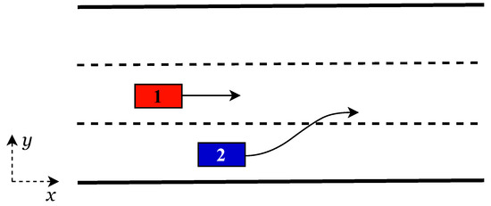
Figure 2. A two-vehicle scenario. There are two vehicles on a three-lane highway. Vehicle 1, in red, is non-reactive in a non-interactive system but reactive in an interactive system and will remain in the center lane. Vehicle 2, in blue, is an SMPC-controlled vehicle, starting in the right, slow lane and later changing into the center lane. The longitudinal and lateral directions are represented by x and y, respectively.

Table 1. Initial settings for a non-interactive two-vehicle scenario.

	${\mathit{x}}_0$	${\mathit{y}}_0$	${\mathit{\psi }}_0$	${\mathit{v}}_0$	${\mathit{y}}_{\mathbf{ref}}$	${\mathit{v}}_{\mathbf{ref}}$
Vehicle 1	50	7.875	0	27	7.875	27
Vehicle 2	72	2.625	0	24	7.875	30

We define the distance $d_{\breve{i},t}$ between EV i and its TV $\breve{i}$ at any iteration $t/T$ (current time t) by the evaluation of the collision-avoidance constraint (12) along the resulting closed-loop trajectories.

$$d_{\breve{i},t}=\sqrt{\frac{{\left(\Delta x_{\breve{i},t}\right)}^2}{s_a^2}+\frac{{\left(\Delta y_{\breve{i},t}\right)}^2}{s_b^2}}$$

(21)

where the distance between EV i and its TV $\breve{i}$ at iteration $t/T$ (time t) in the longitudinal direction is denoted as $\Delta x_{\breve{i},t}$, and its lateral counterpart is $\Delta y_{\breve{i},t}$.

We investigated how the risk parameters influence the distances between vehicles. The risk parameter determines the probability of collision and, thus, controls the distance between two vehicles. Small risk parameters indicate more-aggressive, less-conservative driving with a higher probability of collision and small distances.

To better visualize the influence of the risk parameters on the distances between vehicles, we chose the distance for risk parameter 0.95 as a baseline and evaluated the deviations between the baseline (minuend) and the resulting distances for each of the other risk parameters 0.70, 0.75, 0.80, 0.85, and 0.90. Each risk parameter setting was simulated 100 times, and in each simulation, the initial states of the vehicles were slightly different.

They were generated from a normal distribution with the initial states $\left(x_0,y_0,{\psi }_0,v_0\right)$, as presented in Table 1, as the mean values and a covariance matrix $\mathrm{diag}(0.1,0.01,0,0.01)$. The simulation results are presented in Figure 3, and it was confirmed that the greater the risk parameter of the SMPC-controlled vehicle (the more conservative), the smaller the average distance deviations—meaning larger distances between the two vehicles.

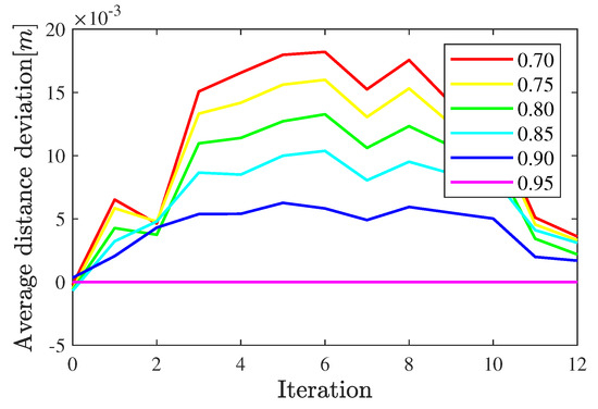
Figure 3. Distance deviations in a non−interactive two−vehicle scenario. The six colored lines represent deviations between the distances for all risk parameters (0.70, 0.75, 0.80, 0.85, 0.90, and 0.95) and the distance for the risk parameter 0.95 during the whole 12 iterations, respectively. The iteration is represented by $t/T$, where t is the time, and T denotes the sampling time.

4.2. The Effects of Risk Parameters on Interactive Systems

In principle, the risk parameter will also determine the distance between vehicles in an interactive system during close interaction. The performance of an individual vehicle depends not only on its own risk parameter but also on the risk parameters of its surrounding vehicles.

4.2.1. The Same vs. Different Risk Parameters

We investigated the state trajectories of two vehicles for different pairs of risk parameters $(p_1,p_2)$, including $(0.70,0.70)$, $(0.70,0.95)$, $(0.95,0.70)$, and $(0.95,0.95)$, based on the two vehicle scenario in Figure 2. Here, both vehicles were reactive and controlled by SMPC. In order to simulate a highly interactive scenario, we slightly adjusted the initial settings of Vehicle 2, as described in Table 1, by (1) moving the longitudinal initial position $x_0$ of Vehicle 2 to 67 $\mathrm{m}$, (2) increasing the initial velocity to 25 ${\mathrm{m}\mathrm{s}}^{-1}$, and (3) decreasing the reference velocity $v_{\mathrm{ref}}$ of Vehicle 2 to 27 ${\mathrm{m}\mathrm{s}}^{-1}$ as summarized in Table 2. We depict the lateral position y of these two vehicles as shown in Figure 4.

Table 2. Initial settings for an interactive two-vehicle scenario.

	${\mathit{x}}_0$	${\mathit{y}}_0$	${\mathit{\psi }}_0$	${\mathit{v}}_0$	${\mathit{y}}_{\mathbf{ref}}$	${\mathit{v}}_{\mathbf{ref}}$
Vehicle 1	50	7.875	0	27	7.875	27
Vehicle 2	67	2.625	0	25	7.875	27

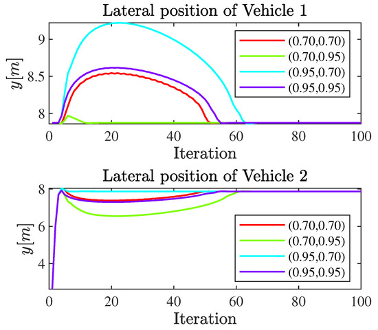
Figure 4. Lateral positions in an interactive two-vehicle scenario. The risk parameter pairs $(p_1,p_2)$ for Vehicle 1 and Vehicle 2 are specified in the legend of the figures.

Figure 4 shows that both Vehicle 1 and Vehicle 2 finally reach their target lanes. We first studied the performance for if both vehicles use the same risk parameter by comparing their lateral positions for risk parameter pairs $(0.70,0.70)$ (red) and $(0.95,0.95)$ (purple). Both vehicles reach their target lane slightly earlier when the common risk parameter is $0.70$. Thus, setting a smaller risk parameter helped the vehicles reach the target lane earlier but not significantly. In total, the resulting trajectories for the risk parameter $(0.70,0.70)$ did not differ too much from those with $(0.95,0.95)$.

We next investigated how the vehicles behave if they use different risk parameters. Comparing the trajectories for the risk parameter pair $(0.70,0.70)$ (red) with that for $(0.95,0.70)$ (blue), we see that if Vehicle 1 chooses a small risk parameter (driving more aggressively), it only slightly adjusts its behavior to avoid potential collisions before reaching the target lane. Vehicle 2 behaves similarly when Vehicle 1 has a greater risk parameter (driving more conservatively). These results are comparable to those for adjusting the risk parameter of Vehicle 2, which can be found in the comparison of the plots for $(0.70,0.70)$ (red) and $(0.70,0.95)$ (green). These results align with the symmetric roles that the two vehicles play in the two-vehicle interactive system, where both vehicles are EVs and treat the other vehicle as a TV.

We summarize the findings for the two-vehicle interactive system as follows:

• When two vehicles have the same risk parameters:
  • Driving more aggressively can help both to reach the target lane slightly earlier.
  • Changing the risk parameters for all vehicles in the same way does not affect the resulting trajectories significantly and only introduces slightly more or less distance between vehicles.
• When two vehicles have different risk parameters:
  • The more aggressive that an EV drives, the fewer collision avoidance adjustments to its behavior are required before reaching the target lane.
  • An EV’s more-aggressive driving style can contribute to reaching its target lane earlier.
  • A TV’s more-conservative driving style can help the EV to reach the target lane earlier with fewer collision avoidance adjustments.

4.2.2. Resolving Conflicts

We now examine the role of the risk parameters in conflict situations. These conflicts were observed in the simulations of the previous subsection where two vehicles could not decide which of them had a higher priority to enter the target lane. This resulted in unnecessarily long lane change durations with oscillations around the target lane. We see that the aggressive vehicle typically dominated the behavior and reached the target lane earlier. When both vehicles had the same risk parameter, target lane and reference velocity, conflict situations often occurred.

We created this kind of conflict by (1) moving Vehicle 2 closer to Vehicle 1 in the longitudinal direction of the initial settings, adjusting the longitudinal initial position $x_0$ of Vehicle 2, as described in Table 2, from 67 to 66 $\mathrm{m}$; and (2) setting the same risk parameter $0.95$ for both vehicles. Thus, the vehicles were initially close to each other, shared the same target velocity of 27 ${\mathrm{m}\mathrm{s}}^{-1}$, and had the same target lane, the center lane; thus, they competed to occupy the center lane.

We investigated how the choice of risk parameters affects vehicle dominance by observing the position and the steering angle $\delta$ of the vehicles for different risk parameter pairs, including $(0.95,0.95)$, $(0.95,0.75)$, and $(0.75,0.95)$ as shown in Figure 5. We mark the time periods where an obvious conflict appears in gray. The oscillating behavior, which is seen in the steering angles in particular, indicates that both vehicles repetitively switched between attempting to approach the target lane and moving away from the target lane to avoid collisions.

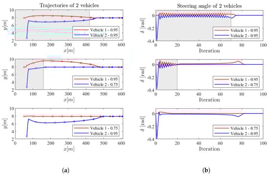
Figure 5. The trajectories and steering angles of Vehicles 1 and 2 for different risk parameter pairs in an interactive scenario. The gray regions in the plots mark time periods of conflict. In sub-figure (a), to display the relative positions of vehicles, we drew the vehicles as small squares every 10 iterations and colored the squares in different shades of red and blue. (a) The trajectories of the vehicles. (b) The steering angles of the vehicles.

Figure 5a displays the trajectories of the vehicles for different risk parameter pairs. Figure 5b shows the corresponding steering angles. When both vehicles used the same risk parameter $0.95$, they remained in conflict until they longitudinally reached around 420 m at approximately iteration 70 and then exited the conflict situation. Reducing the risk parameter of Vehicle 2 from $0.95$ to $0.75$ helped both vehicles escape from the conflict situation even earlier—at around 160 m in the longitudinal direction and after around 20 iterations. Later, Vehicle 2 occupied the target lane most of the time, playing the dominant role (see the trajectories for $(0.95,0.75)$). However, if we reduced the risk parameter of Vehicle 1 from $0.95$ to $0.75$, the conflict situation did not appear anymore, and Vehicle 1 played the dominant role in terms of occupying the target lane (see the trajectories for $(0.75,0.95)$).

Therefore, we can conclude that (1) reducing the risk parameter of one vehicle in the two-vehicle interactive system shortened or fully eliminates conflict; (2) the vehicle with a smaller risk parameter (more aggressive) tended to be the dominant one; additionally, (3) the same amount of risk parameter reduction for Vehicle 1 and Vehicle 2 had different effects on the conflict situations.

4.2.3. Risk Differences

In the previous discussion in Section 4.2.2, we found that maintaining a difference between the risk parameters of the two vehicles helped to either shorten or completely avoid conflict. However, it is also important to know whether the absolute value of the difference matters because this determines how much a vehicle should adjust its behaviors to escape from a conflict situation. Consequently, we decided to further investigate how gradually adjusting the risk parameters of one vehicle affected the resolution of the conflict.

We incrementally increased the risk parameter of Vehicle 1 from $0.75$ to $0.95$, and the risk parameter of Vehicle 2 remained unchanged, $0.95$, resulting in the following risk parameter pairs: $(0.75,0.95)$, $(0.80,0.95)$, $(0.85,0.95)$, $(0.90,0.95)$, and $(0.95,0.95)$. We evaluated the effects of these risk parameter pairs employing two metrics, the Distance Deviation (DD) and State Deviation (SD), introduced as follows:

• DD: We consider the Euclidean distance between the centers of the two vehicles (different from the distance definition in Section 4.1). The DD is defined as the deviation between the Euclidean distances for any risk parameter pair and the Euclidean distance for the risk parameter pair $(0.75,0.95)$.
• SD: The deviation between states and reference states, as defined below:

  $${\mathbf{err}}_{\xi }=\sqrt{\frac{1}{N_{\mathrm{ite}}+1}\sum _{n=0}^{N_{\mathrm{ite}}}{\left({\mathit{\xi }}_n-{\mathit{\xi }}_n^{\mathrm{ref}}\right)}^2}$$

  (22)

  where ${\mathbf{err}}_{\xi }$ (${\mathbf{err}}_{\xi }={\left({\mathrm{err}}_x,{\mathrm{err}}_y,{\mathrm{err}}_{\psi },{\mathrm{err}}_v\right)}^{⊺}$) represents the deviation between the real states ${\mathit{\xi }}_n$ and the corresponding reference states ${\mathit{\xi }}_n^{\mathrm{ref}}$ during all $N_{\mathrm{ite}}$ iterations.

The results for DD and SD are illustrated in Figure 6 and Figure 7, respectively.

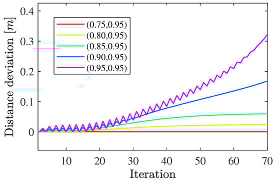
Figure 6. Distance Deviations (DDs) for the vehicles with different pairs of risk parameters, $(0.75,0.95)$, $(0.80,0.95)$, $(0.85,0.95)$, $(0.90,0.95)$, and $(0.95,0.95)$ in an interactive scenario. To better see the details, we enlarged the first 32 iterations of the plot and show them on the top left side of the figure.

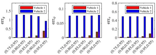
Figure 7. State Deviations (SDs) for the vehicles with different risk parameter pairs, $(0.75,0.95)$, $(0.80,0.95)$, $(0.85,0.95)$, $(0.90,0.95)$, and $(0.95,0.95)$ in an interactive scenario.

In Figure 6, the oscillations reflect conflict where both vehicles are struggling between reaching/maintaining the common target lane and moving away from the target lane to ensure safety, which causes variations in the distances between them. We conclude from the figure that: (1) the greater the risk parameter of Vehicle 1 (the more conservative), the larger the distance between the two vehicles, which is safer; and (2) a smaller risk parameter of Vehicle 1 can help the two-vehicle interactive system escape from the conflict situation earlier as demonstrated by the results that, for the risk parameter pairs $(0.85,0.95)$, $(0.90,0.95)$, and $(0.95,0.95)$, the conflict situations end roughly after 14, 30, and 68 iterations, respectively.

We show the effect of different pairs of the risk parameters on the SD, including the deviations of the lateral position ${\mathrm{err}}_y$, inertial heading ${\mathrm{err}}_{\psi }$, and velocity ${\mathrm{err}}_v$, in Figure 7. A greater risk parameter of Vehicle 1 (more conservative) causes larger state deviations for Vehicle 1, smaller deviations in the lateral positions and velocities for Vehicle 2, and larger inertial heading deviations for Vehicle 2. Therefore, when Vehicle 1 drives more conservatively, Vehicle 2 can benefit from the conservatism more in terms of reaching the target lane and reference velocity (see the first and third sub-figures in Figure 7). In contrast, this results in larger inertial heading deviations for both vehicles (see the second sub-figure in Figure 7) because they are trapped in the conflict situations for a longer time.

The effects of one vehicle’s driving style on the two-vehicle interactive system in conflict situations when the other vehicle drives conservatively are summarized as follows:

• The vehicles benefit from the conservative driving style in terms of safety.
• An aggressive driving style can help the two-vehicle interactive system escape conflict situations.
• A vehicle driving more aggressively tends to reach its target lane and reference velocity earlier.

5. Conclusions and Future Work

In this paper, we introduced a Distributed Stochastic Model Predictive Control (DSMPC) framework for a system of vehicles that are coupled through their interactive controllers. Within this framework, each vehicle is controlled by Stochastic Model Predictive Control (SMPC), and each SMPC-controlled vehicle interacts with its TVs, attempting to drive safely at a certain level through the consideration of probabilistic collision-avoidance constraints. Based on this distributed control framework, we studied the effects of risk parameters, which decide vehicles’ driving styles, on non-interactive and interactive systems and provide insights into how to set risk parameters in a multi-SMPC-vehicle interactive system.

The simulation in non-interactive systems showed that, when an SMPC-controlled vehicle drives more conservatively, with a greater risk parameter, safety is increased. We found the same results in the simulations in interactive systems. Further, in interactive systems, an aggressive vehicle can reach its driving goals earlier, thus, requiring fewer adjustments to its behaviors. An individual vehicle driving conservatively can also help another vehicle to reach its driving goals earlier. Moreover, one vehicle can also influence the whole system by adjusting its own risk parameter. Vehicles might be trapped in conflict situations; therefore, they cannot decide which one has the higher priority to attain one’s driving goals if there are conflicts among the goals. Modifying the risk parameters of one vehicle can help both escape conflict situations; however, the vehicle with a smaller risk parameter tends to dominate the situations.

The results in interactive systems confirmed our hypotheses that the behaviors of one vehicle are not only determined by its own control and influenced by other vehicles’ behaviors but also can influence the performance of the whole system. These results can be generalized to vehicles that are controlled by other controllers in the future.

In our future controller design, incorporating a more realistic prediction of TV’s behaviors into the SMPC optimal-control problem will also be considered. In our current SMPC optimal-control problem, any EV assumes that its TVs will stay in their current lanes and maintain their current velocities. This is overly simplified and might cause huge deviations between the TVs’ real trajectories and the assumed ones from the perspective of the EV. Therefore, methods that provide more precise predictions of TV behaviors are required. Research into this will be performed in the future.

We performed simulations with two vehicles. In the future, we will research more complicated scenarios with multiple vehicles interacting with the surrounding vehicles.

References

- Carvalho, A.; Gao, Y.; Lefevre, S.; Borrelli, F. Stochastic predictive control of autonomous vehicles in uncertain environments. In Proceedings of the 12th International Symposium on Advanced Vehicle Control, Tokyo, Japan, 22–26 September 2014; pp. 712–719. [Google Scholar]
- Soloperto, R.; Köhler, J.; Allgöwer, F.; Müller, M.A. Collision avoidance for uncertain nonlinear systems with moving obstacles using robust Model Predictive Control. In Proceedings of the 2019 18th European Control Conference (ECC), Naples, Italy, 25–28 June 2019; pp. 811–817. [Google Scholar] [CrossRef]
- Suh, J.; Chae, H.; Yi, K. Stochastic Model-Predictive Control for Lane Change Decision of Automated Driving Vehicles. IEEE Trans. Veh. Technol. 2018, 67, 4771–4782. [Google Scholar] [CrossRef]
- Brüdigam, T.; Olbrich, M.; Leibold, M.; Wollherr, D. Combining Stochastic and Scenario Model Predictive Control to Handle Target Vehicle Uncertainty in an Autonomous Driving Highway Scenario. In Proceedings of the 2018 21st International Conference on Intelligent Transportation Systems (ITSC), Maui, HI, USA, 4–7 November 2018; pp. 1317–1324. [Google Scholar] [CrossRef]
- Brüdigam, T.; Olbrich, M.; Wollherr, D.; Leibold, M. Stochastic Model Predictive Control with a Safety Guarantee for Automated Driving. IEEE Trans. Intell. Veh. 2023, 8, 22–36. [Google Scholar] [CrossRef]
- Dang, N.; Brüdigam, T.; Leibold, M.; Buss, M. Combining Event-Based Maneuver Selection and MPC Based Trajectory Generation in Autonomous Driving. Electronics 2022, 11, 1518. [Google Scholar] [CrossRef]
- Heirung, T.A.N.; Paulson, J.A.; O’Leary, J.; Mesbah, A. Stochastic model predictive control—How does it work? Comput. Chem. Eng. 2018, 114, 158–170. [Google Scholar] [CrossRef]
- Kouvaritakis, B.; Cannon, M.; Raković, S.V.; Cheng, Q. Explicit use of probabilistic distributions in linear predictive control. In Proceedings of the UKACC International Conference on Control 2010, Coventry, UK, 7–10 September 2010; pp. 1–6. [Google Scholar] [CrossRef]
- Maroto, J.; Delso, E.; Felez, J.; Cabanellas, J.M. Real-Time Traffic Simulation with a Microscopic Model. IEEE Trans. Intell. Transp. Syst. 2006, 7, 513–527. [Google Scholar] [CrossRef]
- Zambrano-Martinez, J.L.; Calafate, C.T.; Soler, D.; Cano, J.C.; Manzoni, P. Modeling and Characterization of Traffic Flows in Urban Environments. Sensors 2018, 18, 2020. [Google Scholar] [CrossRef]
- Min, W.; Wynter, L. Real-time road traffic prediction with spatio-temporal correlations. Transp. Res. Part C Emerg. Technol. 2011, 19, 606–616. [Google Scholar] [CrossRef]
- Althoff, M.; Stursberg, O.; Buss, M. Model-Based Probabilistic Collision Detection in Autonomous Driving. IEEE Trans. Intell. Transp. Syst. 2009, 10, 299–310. [Google Scholar] [CrossRef]
- Yang, B.; Monterola, C. A simple distributed algorithm for lightless intersection control based on non-linear interactions between vehicles. In Proceedings of the 2017 IEEE 20th International Conference on Intelligent Transportation Systems (ITSC), Yokohama, Japan, 16–19 October 2017; pp. 1–6. [Google Scholar] [CrossRef]
- Dai, L.; Xia, Y.; Gao, Y.; Kouvaritakis, B.; Cannon, M. Cooperative distributed stochastic MPC for systems with state estimation and coupled probabilistic constraints. Automatica 2015, 61, 89–96. [Google Scholar] [CrossRef]
- Dai, L.; Xia, Y.; Gao, Y.; Cannon, M. Distributed Stochastic MPC of Linear Systems with Additive Uncertainty and Coupled Probabilistic Constraints. IEEE Trans. Autom. Control 2017, 62, 3474–3481. [Google Scholar] [CrossRef]
- Zhao, G.; Yang, S. Distributed stochastic MPC for linear systems with probabilistic constraints and quantisation. IET Control Theory Appl. 2020, 14, 396–404. [Google Scholar] [CrossRef]
- Dunbar, W.B.; Murray, R.M. Distributed receding horizon control for multi-vehicle formation stabilization. Automatica 2006, 42, 549–558. [Google Scholar] [CrossRef]
- Dunbar, W.B.; Caveney, D.S. Distributed Receding Horizon Control of Vehicle Platoons: Stability and String Stability. IEEE Trans. Autom. Control 2012, 57, 620–633. [Google Scholar] [CrossRef]
- Zheng, Y.; Li, S.E.; Li, K.; Borrelli, F.; Hedrick, J.K. Distributed Model Predictive Control for Heterogeneous Vehicle Platoons Under Unidirectional Topologies. IEEE Trans. Control Syst. Technol. 2017, 25, 899–910. [Google Scholar] [CrossRef]
- Liu, P.; Kurt, A.; Ozguner, U. Distributed Model Predictive Control for Cooperative and Flexible Vehicle Platooning. IEEE Trans. Control Syst. Technol. 2019, 27, 1115–1128. [Google Scholar] [CrossRef]
- Gao, Y.; Lin, T.; Borrelli, F.; Tseng, E.; Hrovat, D. Predictive Control of Autonomous Ground Vehicles with Obstacle Avoidance on Slippery Roads. In Proceedings of the ASME 2010 Dynamic Systems and Control Conference, Cambridge, MA, USA, 12–15 September 2010. [Google Scholar] [CrossRef]
- Levinson, J.; Askeland, J.; Becker, J.; Dolson, J.; Held, D.; Kammel, S.; Kolter, J.Z.; Langer, D.; Pink, O.; Pratt, V.; et al. Towards fully autonomous driving: Systems and algorithms. In Proceedings of the 2011 IEEE Intelligent Vehicles Symposium (IV), Baden-Baden, Germany, 5–9 June 2011; pp. 163–168. [Google Scholar] [CrossRef]
- Carvalho, A.; Gao, Y.; Gray, A.; Tseng, H.E.; Borrelli, F. Predictive control of an autonomous ground vehicle using an iterative linearization approach. In Proceedings of the 16th International IEEE Conference on Intelligent Transportation Systems (ITSC 2013), Hague, The Netherlands, 6–9 October 2013; pp. 2335–2340. [Google Scholar] [CrossRef]
- Kong, J.; Pfeiffer, M.; Schildbach, G.; Borrelli, F. Kinematic and dynamic vehicle models for autonomous driving control design. In Proceedings of the 2015 IEEE Intelligent Vehicles Symposium (IV), Seoul, Republic of Korea, 28 June–1 July 2015; pp. 1094–1099. [Google Scholar]
- Brüdigam, T.; Olbrich, M.; Wollherr, D.; Leibold, M. Stochastic Model Predictive Control with a Safety Guarantee for Automated Driving: Extended Version. arXiv 2020, arXiv:2009.09381. [Google Scholar] [CrossRef]
- Lorenzen, M.; Dabbene, F.; Tempo, R.; Allgöwer, F. Constraint-Tightening and Stability in Stochastic Model Predictive Control. IEEE Trans. Autom. Control 2017, 62, 3165–3177. [Google Scholar] [CrossRef]
- Grüne, L.; Pannek, J. Nonlinear Model Predictive Control: Theory and Algorithms, 2nd ed.; Communications and Control Engineering; Springer: Cham, Switzerland, 2017. [Google Scholar]
Disclaimer/Publisher’s Note: The statements, opinions and data contained in all publications are solely those of the individual author(s) and contributor(s) and not of MDPI and/or the editor(s). MDPI and/or the editor(s) disclaim responsibility for any injury to people or property resulting from any ideas, methods, instructions or products referred to in the content. |
© 2023 by the authors. Licensee MDPI, Basel, Switzerland. This article is an open access article distributed under the terms and conditions of the Creative Commons Attribution (CC BY) license (https://creativecommons.org/licenses/by/4.0/).