NGDCNet: Noise Gating Dynamic Convolutional Network for Image Denoising

Abstract

Deep convolution neural networks (CNNs) have become popular for image denoising due to their robust learning capabilities. However, many methods tend to increase the receptive field to improve performance, which leads to over-smoothed results and loss of critical high-frequency information such as edges and texture. In this research, we introduce an innovative end-to-end denoising network named the noise gating dynamic convolutional network (NGDCNet). By integrating dynamic convolution and noise gating mechanisms, our approach effectively reduces noise while retaining finer image details. Through a series of experiments, we conduct a comprehensive evaluation of NGDCNet by comparing it quantitatively and visually against state-of-the-art denoising methods. Additionally, we provide an ablation study to analyze the contributions of dynamic convolutional blocks and noise gating blocks. Our experimental findings demonstrate that NGDCNet excels in noise reduction while preserving essential texture information.

1. Introduction

Due to the intricate acquisition processes involving capturing, transmitting, and compressing images through digital devices, the acquired images are susceptible to variations in lighting conditions and sensor noise [1]. Image noise, which manifests as random fluctuations in brightness or color, poses a challenge to image observation and accurate information extraction in image processing. The detrimental effects of noise can impact a range of image processing tasks, such as video processing, image analysis, and segmentation, potentially leading to erroneous judgments [2]. In response to this challenge, image denoising techniques have been devised.

Image denoising techniques are specifically designed to mitigate the impact of noise. They aim to remove unwanted noise, allowing for the accurate representation and storage of a clean image based on a degenerate model $y=c+n$, where c represents a potentially clean image, n is the noise, and y corresponds to the noisy image [3]. Building on this understanding, filter methods have gained significant traction for effectively suppressing noise in noisy images [4]. Spatial domain filters, for example, employ pixel averaging within specific regions to enhance the quality of predicted images [5]. Furthermore, combining compensation functions and bilateral filtering can augment edges to extract more detailed information, thus bolstering denoising efficiency [6]. Additionally, based on image characteristics, transforming the image to the transform domain has proven effective in noise removal [7]. Block Matching 3D (BM3D) leverages block comparability assessments to perform transform domain filtering in image denoising [8]. This process involves grouping similar patches, condensing the 3D transform domain for collaborative filtering, and then reconstructing the original position by aggregating these acquired patches. Given BM3D’s outstanding performance, various variants have been developed for denoising tasks [9]. Moreover, perceptual concepts have been employed to extract noisy information from a given noisy image, contributing to denoising techniques [10]. Total variation, an approach involving minimizing the total variation of an image, was introduced in image denoising and has demonstrated effectiveness [11]. Additionally, the partial differential equation (PDE) algorithm treats the denoising process as solving an equation through multiple iterations, approaching a solution close to a potentially clean image [12]. Due to PDE’s properties, its variants are advantageous in preserving edge and texture information during image denoising [13]. Another approach, weighted kernel paradigm minimization (WNNM), utilizes low-rank clustering correlation concepts to filter noise and recover high-quality images [14]. Other popular denoising methods encompass Markov random fields [15] and gradient methods [16].

With the rapid advancement of deep learning, particularly the widespread adoption of convolutional neural networks (CNNs) known for their high speed of execution and strong learning capabilities, the domain of image denoising has witnessed a significant transformation [17]. Over the past decade, numerous CNN-based denoising methods have surfaced, including IRCNN [18], DnCNN [19], and complex-valued deep CNN [20]. However, a common challenge faced by these methods is the depth of the network which makes training arduous. To address the training issue, Tian et al. [21] introduced an enhanced convolutional neural denoising network (ECNDNet), incorporating residual learning [22], dilation convolution, and batch normalization [23] to expedite network convergence. Additionally, combining CNNs with other deep learning techniques has shown promise in achieving improved denoising results. For instance, Zhao et al. [24] proposed a hybrid denoising model that integrates a transformer encoder and a convolutional decoder network, effectively leveraging the strengths of both networks for the successful denoising of real images. Kumwilaisak et al. [25] devised a novel approach based on deep CNNs and multidirectional long short-term memory networks to eliminate pine tree noise from images. Moreover, the fusion of unsupervised learning with CNNs has paved the way for even more versatile applications. Pang et al. [26] introduced an unsupervised deep noise reducer to tackle the issue of overfitting due to the lack of real images.

Despite the success of various deep CNN-based methods in image denoising, many recent approaches [27] aim to achieve enhanced performance by increasing the receptive field. However, this potentially leads to over-smoothed results and loss of critical high-frequency information such as edges and textures [28,29]. Therefore, this paper introduces a novel denoising method called NGDCNet to achieve effective image denoising while being able to better preserve the texture information of the image. The method is based on deep CNN and replaces the traditional static convolution with dynamic convolution [30]. This transformation can aggregate dynamic kernels during the convolution operation to fully utilize the correlation within the deep features [30], giving the network the ability to recover complex high-frequency information. However, dynamic convolution is sensitive to noise [31]. Therefore, this paper proposes a residue-like structure that combines a noise gating mechanism with skip connections. This residual-like structure can effectively control the propagation of low-level features to higher levels through the learning process, thus reducing the interference of low-level redundant features on dynamic convolution.

The main contributions of this study can be summarized as follows:

• We propose a residual-like structure that combines the noise gating mechanism with skip connections. The residual-like structure effectively refines the ordinary skip connection.
• We combine dynamic convolution and noise gating mechanisms to propose a simple and effective network architecture that can achieve excellent denoising performance.

This paper follows a structured organization. Section 2 provides a comprehensive review of the related work. Section 3 presents our denoising framework in detail. In Section 4, we conduct a series of comparative experiments to showcase the effectiveness of the proposed denoising methods. Section 5 concludes the work presented in this paper.

2. Related Work

Recently, denoising models founded on CNNs have garnered significant attention, largely owing to their outstanding performance [32,33]. CNN-based denoising models typically involve a manageable number of hyperparameters, reducing the need for extensive manual intervention and often ensuring relatively fast operation speeds [34,35,36]. One notable denoising model is the denoising CNN proposed by Zhang et al. [19] (DnCNN). By integrating residual learning [22] and batch normalization [23], the training process of DnCNN is accelerated, significantly improving denoising performance. Building upon DnCNN, Helou et al. [37] introduced a blind universal image fusion denoiser (BUIFD) that incorporates a noise level estimation network into the model. This addition allows BUIFD to process images with a broad range of noise levels effectively. Zhang et al. [18] designed the image recovery CNN (IRCNN) for blind image denoising, utilizing dilated convolution [38] to expand the receptive field. A fast and flexible denoising network (FFDNet) was proposed in [39] for generalized image denoising to address inflexible denoising models. FFDNet utilizes an adjustable noise level map as a network input, enabling it to handle various noise levels and effectively remove spatially varying noise.

Furthermore, Ref. [40] introduced a deep residual CNN (DRCNN) for image denoising, leveraging residual learning to enhance denoising performance. Xu et al. [41] developed a noise fusion CNN (NFCNN) with a multi-level architecture for image denoising, incorporating two branches to predict potentially clean and residual images, which are then fused to generate results for the subsequent stage. DeamNet [42] introduced adaptive consistency prior (ACP) to augment traditional consistency priors. Li et al. [43] proposed an all-in-one image recovery network (AirNet) capable of recovering various degraded images using a single network for unknown corruptions, rendering it flexible and effective for image recovery. DRUNet [44], a combination of U-Net and ResNet [22], offers pre-trained denoisers that are both flexible and highly effective, showcasing state-of-the-art denoising performance. Despite their impressive performance, these models tend to be overly complex for practical denoising scenarios. A robust deformable denoising CNN (RDDCNN) was proposed by Tian et al. [45]. The RDDCNN comprises three blocks: the deformable block (DB), the enhanced block (EB), and the residual block (RB). The DB extracts more representative noise features by utilizing a deformable learnable kernel and a stacked convolutional architecture based on the relationship of surrounding pixels. The EB promotes contextual interactions through a novel combination of dilated convolution, convolutional layers, batch normalization, and ReLU, enhancing the learning capacity of the RDDCNN. To address the challenge of long-term dependencies, the RB is employed to augment the ability of shallow layers to remember deep-layer information, facilitating the construction of clean images. Shen et al. [31] introduced an efficient denoising network named ADFNet, leveraging improved dynamic convolution. In particular, Ref. [31] devised a spatially enhanced kernel generation (SEKG) module to enhance dynamic convolution. This enhancement facilitates the learning of spatial context information while maintaining minimal computational complexity. Tian et al. [46] introduced a multistage image denoising CNN called MWDCNN which operates through three stages: dynamic convolution block (DCB), two cascaded wavelet transforms with enhancement blocks (WEBs), and a residual block (RB). The DCB utilizes dynamic convolution to adaptively adjust the parameters of multiple convolutions, achieving a balance between denoising performance and computational cost. WEB leverages a combination of signal processing techniques such as wavelet transforms and discriminative learning to suppress noise, consequently recovering more intricate information during image denoising. To further eliminate redundant features, RB is employed to refine the obtained features, enhancing denoising and enabling the reconstruction of clean images through an improved residual dense architecture.

3. Proposed Method

In this subsection, we present our proposed denoising network model, comprising noise gating dynamic convolutional block (NGDCB) and residual block (RB). NGDCB is composed of two crucial components: dynamic convolution block (DCB) [30] and noise gating block (NGB). Our main focus for improving the image denoising effect revolves around these two blocks: DCB and NGB.

To elaborate, DCB plays a pivotal role in enabling the network to recover intricate high-frequency information effectively. It achieves this by incorporating five stacked dynamic convolutions. On the other hand, NGB effectively controls the flow of lower features to higher levels, optimizing skip connections. In the subsequent sections, we provide a detailed description of the network model, its constituent blocks, and the pertinent functions involved.

3.1. Network Model

This paper introduces a network model named NGDCNet, which is composed of NGDCB and RB as depicted in Figure 1. To provide a clearer representation of the operational process, we present it in the following equation:

$$I_c=NGDCNet\left(I_n\right)=RB\left(NGDCB\left(NGDCB\left(NGDCB\left(I_n\right)\right)\right)\right)$$

(1)

where $I_c$ denotes the predicted clean image, $NGDCNet$ denotes the function of NGDCNet, and $I_n$ denotes the given noisy image. Also, $RB$ and $NGDCB$ are functions of RB and NGDCB, respectively.

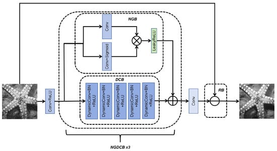
Figure 1. Network model of the proposed NGDCNet.

3.2. Loss Function

To enhance the credibility of our denoising network, we chose the $L_1$ as the loss function for training the model parameters. This process can be expressed using the following formula:

$$L_1\left(\theta \right)=\frac{1}{N}\sum _{i=1}^N|y_i-NGDCNet\left(x_i\right)|$$

(2)

where $x_i$ and $y_i$ denote the i-th noisy images and given clean images, respectively, and $\theta$ denotes the parameters in training the denoising model. In addition, N stands for the total of noisy images.

3.3. Noise Gating Dynamic Convolutional Block

3.3.1. Noise Gating Block

In general, residual learning is usually implemented using simple skip connections. This can be used in many tasks [22]. However, during the denoising process, skip connections may be counterproductive by passing lower redundant features to higher levels. Therefore, this study utilizes a noise gating mechanism [47,48], which controls the transmission of trivial features by learning spatial feature correlations. The noise gating mechanism is obtained as follows:

$$Gat{e}_{i,j}=\sum _{i=1}^H\sum _{j=1}^W{W}_g·I$$

(3)

$$Feature{s}_{i,j}=\sum _{i=1}^H\sum _{j=1}^W{W}_f·I$$

(4)

$$Outpu{t}_{i,j}=\delta (Gat{e}_{i,j}\odot \theta \left(Feature{s}_{i,j}\right))$$

(5)

where $\delta$ is the LeakyReLU activation function, and $\theta$ is the sigmoid function.

In this paper, we combine the noise gating mechanism with a skip connection to form a residual-like structure named NGB. The NGB comprises two branches: one with a standard convolutional layer denoted as Conv and the other with Conv + Sigmoid. These branches individually process the input features, and their results are combined through element-wise multiplication (represented as ⊗ in Figure 1. Subsequently, the combined features undergo processing by LeakyReLU and are then summed with the output from $DCB$. To provide a clearer representation of this process, we use the following equation to describe it:

$$O_{NGB}=NGB\left(I\right)=LR(C\left(I\right)\ast CS\left(I\right))$$

(6)

where $LR$ denotes LeakyReLU, $CS$ denotes $3\times 3$ kernel size of Conv + Sigmoid, and $NGB$ denotes noise gating convolutional block. For the first $NGB$, I denotes the image disturbed by noise. For the middle stacked $NGB$, I is the result of summing the outputs of the previous $NGB$ and the $DCB$. $O_{NGB}$ is the output of $NGB$.

3.3.2. Dynamic Convolutional Block

The main component consists of three stacked DCBs, with each DCB comprising five dynamic convolutional layers [30]. These are primarily aimed at extracting finer high-frequency information. Specifically, the first layer consists of a standard convolutional layer and ReLU to extract lower-level features. It has a kernel size of $3\times 3$, with input and output channels of 1 and 64, respectively (or 3 for color image denoising). ReLU is responsible for transforming linear features into nonlinear features. Each DCB consists of five DynamicConv + BN + ReLU layers. Each DCB has both input and output channels set at 64 where the end of each DCB is connected to a skip connection improved by NGB. To provide a clearer representation of this process, we use the following equation to describe it:

$$\begin{array}{cc}\hfill O_{DCB}& =DCB\left(I\right)\hfill \\ & =DCBR\left(DCBR\right(DCBR\left(DCBR\right(DCBR\left(CR\right(I\left)\right)\left)\right)\left)\right)\hfill \end{array}$$

(7)

where $CR$ denotes the $3\times 3$ kernel size of Conv + ReLU and $DCBR$ denotes the $3\times 3$ kernel size of DynamicConv + BN + ReLU. For the first $DCB$, I denotes the image disturbed by noise. For the middle stacked $DCB$, I is the result of summing the outputs of the previous $NGB$ and the $DCB$. $O_{DCB}$ is the output of $DCB$.

3.4. Residual Block

The residual block is employed to construct a latent clean image. It encompasses a single convolutional layer, denoted as Conv in Figure 1. The residual block employs a residual learning operation to eliminate noise from the provided image in the following manner:

$$I_c=RB\left(C\left(O_{NGDCB}\right)\right)=I_n-\left(C(O_{DCB}+O_{NGB})\right)$$

(8)

where − is the ⊖ in Figure 1. C means that the kernel size of the convolution is $3\times 3$. $O_{NGDCB}$ is the output of the last $NGDCB$.

4. Experiments

4.1. Datasets and Implementation Details

For grayscale Gaussian image denoising, the train set was established by converting the 432 training images sourced from the BSD68 [49] dataset into grayscale images. For the subsequent evaluation, we utilized two distinct test sets. The first test set comprised 68 test images from BSD68, while the second test set was derived from the Set12 [50] dataset. We compared the peak signal-to-noise ratio (PSNR) [51] and structural similarity (SSIM) [52] under varying noise conditions, benchmarking these results against the outcomes obtained from other denoising methods.

For color Gaussian image denoising, we utilized the same 432 training images from the BSD68 dataset. We constructed two test sets: the first set consisted of 68 test images from BSD68, and the second set was derived from the Set5 [53] dataset. Within this context, we performed a comparative analysis by comparing the PSNR and SSIM under diverse noise conditions, analyzing them in relation to various denoising methods.

The hardware platform for this experiment is a Tesla V100 with 16 GB of RAM; the software is Ubuntu18.04.5, CUDA10.1, python3.7.0; the deep learning framework is Pytorch1.5.0; the batch processing is 4; the Adam algorithm is used to update the gradient; the initial learning rate is $0.001$, and the learning rate decreases with the number of training times.

4.2. Evaluation Metrics

After image denoising, image quality evaluation criteria are usually introduced to evaluate the merits of denoising models. In this paper, PSNR and SSIM are used for evaluation and analysis.

4.2.1. PSNR

PSNR is a metric that quantifies the ratio of the maximum possible power of a signal to the power of the noise in an image. A higher PSNR value implies that the image has a greater proportion of signal compared to noise, resulting in better image quality. It is measured in decibels (dB), and in general, if the PSNR exceeds 40 dB, the image quality is very good. If $MA{X}_i$ denotes the maximum gray value and $MSE$ [54] denotes the mean square error, the $PSNR$ is expressed by the following formula:

$$PSNR=10{\log }_{10}(\frac{MA{X}_i^2}{MSE})$$

(9)

$$MSE=\frac{1}{M\times N}\sum _{i=0}^{M-1}\sum _{j=0}^{N-1}{[c(i,j)-n(i,j)]}^2$$

(10)

where $M\times N$ is the total number of pixel values of the two images, respectively, $c(i,j)$ is the real clean image, and $n(i,j)$ is the denoised image. A smaller $MSE$ value means that the difference between the predicted value and the real value is smaller, which implies that the denoising effect is better and the performance of the model is better.

4.2.2. SSIM

SSIM measures the similarity of two images and is a common metric for image quality assessment [55]. Assuming input images X and Y, the $SSIM$ of images X and Y is computed as follows:

$$SSIM(X,Y)=\frac{(2{\mu }_X{\mu }_Y+a_1)(2{\sigma }_{XY}+a_2)}{({\mu }_X^2+{\mu }_Y^2+a_3)({\sigma }_X^2+{\sigma }_Y^2+a_4)}$$

(11)

where ${\mu }_X$ and ${\mu }_Y$ are the standard deviation of X and Y, ${\sigma }_X^2$ and ${\sigma }_Y^2$ are the variance of X and Y, ${\sigma }_{XY}$ is the covariance of X and Y, and $a_1$, $a_2$, $a_3$ and $a_4$ are constants. Generally, the SSIM value is in the range of $[-1,1]$, and the larger the SSIM value, the better the image denoising.

4.3. Experimental Result and Analysis

4.3.1. Comparison with State-of-the-Art Denoising Methods

• Gray Gaussian Image Denoising

To evaluate the effectiveness of the proposed NGDCNet for denoising gray Gaussian noisy images, we compared it with five existing methods: DnCNN [19], FFDNet [39], IRCNN [18], DRUNet [56], and NIFBGDNet [57]. The image blind denoising experiments, presented in Table 1, involved testing these methods across three noise levels (15, 25, and 50). The quantitative results demonstrate that NGDCNet achieved notably high PSNR and SSIM values on both datasets, indicating its superior denoising performance.

Table 1. Average PSNR (dB) and SSIM of different methods on BSD68 with noise levels of 15, 25, and 50.

Methods	15		25		50
	PSNR	SSIM	PSNR	SSIM	PSNR	SSIM
FFDNet	31.43	0.8862	29.04	0.8246	26.18	0.7205
DnCNN	31.61	0.8866	29.15	0.8242	26.22	0.7161
DRUNet	31.90	0.8951	29.47	0.8369	26.58	0.7376
IRCNN	31.63	0.8881	29.14	0.8246	26.18	0.7167
NIFBGDNet	31.19	0.8754	28.82	0.8101	25.98	0.7008
NGDCNet	32.60	0.9195	30.85	0.8869	28.28	0.8040

The results presented in Table 1 demonstrate the superior performance of NGDCNet in terms of PSNR and SSIM values when compared to the five other methods across the three distinct noise levels. Particularly at a noise level of $\sigma =15$, our model exhibited substantially higher PSNR and SSIM scores than the other methods. Impressively, even at a higher noise level ($\sigma =50$), our model consistently maintained outstanding performance. It is worth noting that our model achieved these impressive results without needing an additional training set. This robust performance across varying noise levels underscores the NGDCNet’s formidable capability to recover corrupted images effectively.

Table 2 and Table 3 display the test results of NGDCNet in comparison to the other five methods on the Set12 dataset. The results in Table 2 show that NGDCNet consistently achieves higher average PSNR at noise levels of 15, 25, and 50 compared to the other models. Particularly noteworthy is the performance at a noise level of 50, where NGDCNet’s PSNR value surpasses the second-ranked method by $1.04$ dB. These results underscore the exceptional denoising effect of NGDCNet at low and medium noise levels, demonstrating its superior ability to maintain image quality in such scenarios. Even at higher noise levels, NGDCNet maintains excellent performance, showcasing its effectiveness across various noise conditions.

Table 2. Average PSNR (dB) of different methods on Set12 with noise levels of 15, 25, and 50.

Images	C.man	House	Peppers	Starfish	Monarch	Airplane	Parrot	Lena	Barbara	Boat	Man	Couple	Average
Noise Level	15
FFDNet	31.95	34.64	32.54	31.55	32.62	31.21	31.46	34.38	31.83	32.15	32.19	32.17	32.39
DnCNN	32.14	34.96	33.09	31.92	33.08	31.54	31.64	34.52	32.03	32.36	32.37	32.38	32.67
DRUNet	32.91	35.83	33.56	32.44	33.61	31.99	32.13	34.93	33.44	32.71	32.61	32.78	33.25
IRCNN	32.53	34.88	33.21	31.96	32.98	31.66	31.88	34.50	32.41	32.36	32.36	32.37	32.76
NIFBGDNet	31.44	34.52	32.66	31.56	32.63	31.08	31.21	34.27	31.42	32.10	32.14	31.99	32.25
NGDCNet	32.96	35.59	33.86	32.25	33.51	32.51	32.68	35.24	32.89	32.76	33.28	33.21	33.40
Noise Level	25
FFDNet	29.76	32.83	30.37	29.00	30.10	28.80	29.19	32.33	29.42	30.02	29.96	29.91	30.14
DnCNN	30.03	33.04	30.73	29.24	30.37	29.06	29.36	32.40	29.67	30.19	30.06	30.05	30.35
DRUNet	30.61	33.93	31.22	29.88	30.89	29.35	29.72	32.97	31.23	30.58	30.30	30.56	30.94
IRCNN	30.12	33.02	30.81	29.21	30.20	29.05	29.47	32.40	29.93	30.17	30.02	30.05	30.37
NIFBGDNet	29.45	32.60	30.26	28.97	30.04	28.67	29.02	32.13	28.97	29.91	29.87	29.65	29.96
NGDCNet	31.19	34.05	32.28	30.14	32.31	30.68	30.94	33.79	30.95	31.57	31.80	31.64	31.78
Noise Level	50
FFDNet	27.04	29.90	27.20	25.49	26.76	25.68	26.36	29.39	25.82	27.12	27.17	26.84	27.06
DnCNN	27.26	29.91	27.35	25.60	26.85	25.82	26.48	29.34	26.32	27.18	27.17	26.87	27.18
DRUNet	27.80	31.26	27.87	26.49	27.31	26.08	26.92	30.15	28.16	27.66	27.46	27.59	27.90
IRCNN	27.16	29.90	27.33	25.48	26.66	25.78	26.48	29.36	26.17	27.17	27.14	26.86	27.12
NIFBGDNet	26.75	29.40	26.82	25.45	26.59	25.48	26.19	29.07	25.43	26.92	27.00	26.45	26.80
NGDCNet	29.03	28.23	30.06	28.49	27.49	28.39	28.85	30.54	28.10	29.53	29.47	29.10	28.94

Table 3. Average SSIM of different methods on Set12 with noise levels of 15, 25, and 50.

Images	C.man	House	Peppers	Starfish	Monarch	Airplane	Parrot	Lena	Barbara	Boat	Man	Couple	Average
Noise Level	15
FFDNet	0.9075	0.8830	0.9069	0.9085	0.9459	0.9034	0.8999	0.8975	0.9122	0.8552	0.8762	0.8777	0.8978
DnCNN	0.9025	0.8866	0.9103	0.9121	0.9480	0.9055	0.8995	0.8996	0.9162	0.8594	0.8795	0.8807	0.9000
DRUNet	0.9168	0.9080	0.9155	0.9184	0.9537	0.9116	0.9100	0.9077	0.9310	0.8690	0.8852	0.8908	0.9098
IRCNN	0.9113	0.8831	0.9107	0.9123	0.9477	0.9064	0.9039	0.8985	0.9175	0.8589	0.8782	0.8785	0.9006
NIFBGDNet	0.8895	0.8795	0.9060	0.9074	0.9427	0.8999	0.8938	0.8952	0.9049	0.8543	0.8739	0.8710	0.8932
NGDCNet	0.9217	0.9030	0.9305	0.9267	0.9526	0.9257	0.9290	0.9128	0.9277	0.8777	0.9065	0.9044	0.9182
Noise Level	25
FFDNet	0.8711	0.8585	0.8750	0.8618	0.9166	0.8669	0.8592	0.8683	0.8689	0.8059	0.8194	0.8247	0.8580
DnCNN	0.8659	0.8613	0.8766	0.8658	0.9177	0.8681	0.8584	0.8689	0.8757	0.8109	0.8215	0.8286	0.8599
DRUNet	0.8828	0.8718	0.8857	0.8764	0.9288	0.8759	0.8692	0.8833	0.9045	0.8240	0.8294	0.8472	0.8732
IRCNN	0.8715	0.8591	0.8775	0.8646	0.9171	0.8670	0.8608	0.8684	0.8763	0.8088	0.8194	0.8268	0.8598
NIFBGDNet	0.8522	0.8541	0.8700	0.8596	0.9097	0.8610	0.8520	0.8626	0.8555	0.8006	0.8134	0.8131	0.8503
NGDCNet	0.8978	0.8808	0.9121	0.8911	0.9440	0.9030	0.9023	0.8916	0.8988	0.8533	0.8785	0.8757	0.8941
Noise Level	50
FFDNet	0.8113	0.8215	0.8115	0.7715	0.8525	0.7982	0.7977	0.8148	0.7569	0.7176	0.7235	0.7244	0.7834
DnCNN	0.8044	0.8164	0.8065	0.7715	0.8484	0.7935	0.7934	0.8088	0.7744	0.7176	0.7204	0.7245	0.7816
DRUNet	0.8267	0.8412	0.8271	0.8013	0.8724	0.8093	0.8098	0.8392	0.8423	0.7440	0.7372	0.7651	0.8096
IRCNN	0.8028	0.8159	0.8044	0.7675	0.8454	0.7953	0.7953	0.8096	0.7704	0.7155	0.7193	0.7238	0.7804
NIFBGDNet	0.7901	0.8032	0.7979	0.7640	0.8388	0.7820	0.7842	0.8000	0.7309	0.7035	0.7111	0.6993	0.7671
NGDCNet	0.8161	0.6730	0.8538	0.8603	0.7955	0.8369	0.8379	0.7974	0.8225	0.7916	0.8039	0.8075	0.8083

In Table 3, it is apparent that NGDCNet achieves higher SSIM values than the other methods at noise levels of 15 and 25. While at a noise level of 50, the SSIM value of NGDCNet is slightly lower than that of DRUNet, indicating NGDCNet’s ability to maintain image structure effectively in most situations.

• Color Gaussian Image Denoising

Table 4 displays the test results of NGDCNet in comparison with other methods on the CBSD68 [49] dataset. It is evident that NGDCNet exhibits remarkable performance in color Gaussian image denoising. NGDCNet consistently outperforms other methods, as indicated by its higher PSNR and SSIM values across various noise levels. Notably, NGDCNet achieves an impressive SSIM of $0.8717$ at a noise level of 50, showcasing its ability to preserve image structure even under very high noise conditions.

Table 4. Average PSNR (dB) and SSIM of different methods on CBSD68 with noise levels of 15, 25, and 50.

Methods	15		25		50
	PSNR	SSIM	PSNR	SSIM	PSNR	SSIM
FFDNet	33.88	0.9290	31.22	0.8821	27.97	0.7887
DnCNN	33.90	0.9290	31.24	0.8830	27.95	0.7896
DRUNet	34.30	0.9344	31.69	0.8926	28.51	0.8103
IRCNN	33.87	0.9285	31.18	0.8824	27.88	0.7898
NIFBGDNet	33.67	0.9260	31.00	0.8769	27.70	0.7767
NGDCNet	35.34	0.9562	33.34	0.9339	29.85	0.8717

Table 5 demonstrates the test results of NGDCNet compared to other methods on the Set5 dataset. These results reveal that NGDCNet consistently achieves higher average PSNR and SSIM values compared to other methods at noise levels of 15 and 25. This underscores the exceptional performance of NGDCNet, particularly in situations involving low to medium noise levels. Impressively, at the noise level of 50, NGDCNet achieves a PSNR value of $30.52$ dB, surpassing DRUNet by $0.65$ dB.

Table 5. Average PSNR (dB) of different methods on Set5 with noise levels of 15, 25, and 50.

Images	Baby	Bird	Butterfly	Head	Woman	Average
Noise Level	15
FFDNet	35.48	35.45	33.65	31.67	35.31	34.31
DnCNN	35.39	34.62	33.61	31.35	35.25	34.05
DRUNet	35.79	35.93	34.85	32.13	35.81	34.90
IRCNN	35.47	35.28	33.64	31.63	35.27	34.26
NIFBGDNet	35.28	34.60	33.36	31.18	35.21	33.93
NGDCNet	36.88	35.91	34.84	31.24	36.86	35.15
Noise Level	25
FFDNet	33.31	33.00	31.04	30.30	32.91	32.11
DnCNN	33.21	32.33	31.08	30.16	32.79	31.91
DRUNet	33.67	33.57	32.31	30.65	33.44	32.73
IRCNN	33.22	32.69	30.95	30.28	32.77	31.98
NIFBGDNet	33.04	32.20	30.84	30.07	32.72	31.78
NGDCNet	35.24	34.13	32.87	30.95	34.74	33.59
Noise Level	50
FFDNet	30.52	29.41	27.77	28.70	29.80	29.24
DnCNN	30.28	28.83	27.69	28.51	29.48	28.96
DRUNet	31.01	30.17	28.79	29.06	30.34	29.87
IRCNN	30.34	29.03	27.54	28.54	29.55	29.00
NIFBGDNet	30.04	28.77	27.44	28.45	29.40	28.82
NGDCNet	31.68	30.75	29.67	29.54	30.98	30.52

Table 6 further supports the superiority of NGDCNet, with its SSIM values outperforming other methods across all three noise levels. Even at the noise level of 50, the SSIM value of NGDCNet exceeds the second-ranked method by $0.0336$, indicating NGDCNet’s ability to effectively preserve image structure under varying noise conditions.

Table 6. Average SSIM of different methods on Set5 with noise levels of 15, 25, and 50.

Images	Baby	Bird	Butterfly	Head	Woman	Average
Noise Level	15
FFDNet	0.9259	0.9384	0.9573	0.8116	0.9531	0.9173
DnCNN	0.9235	0.9312	0.9560	0.7938	0.9521	0.9113
DRUNet	0.9309	0.9466	0.9641	0.8320	0.9580	0.9263
IRCNN	0.9261	0.9377	0.9558	0.8069	0.9521	0.9157
NIFBGDNet	0.9226	0.9264	0.9540	0.7808	0.9521	0.9072
NGDCNet	0.9583	0.9726	0.9730	0.8761	0.9723	0.9505
Noise Level	25
FFDNet	0.8936	0.9080	0.9379	0.7427	0.9314	0.8827
DnCNN	0.8898	0.8994	0.9360	0.7372	0.9281	0.8781
DRUNet	0.9008	0.9229	0.9501	0.7663	0.9394	0.8959
IRCNN	0.8918	0.9037	0.9342	0.7455	0.9276	0.8806
NIFBGDNet	0.8872	0.8910	0.9348	0.7269	0.9274	0.8735
NGDCNet	0.9402	0.9567	0.9614	0.8632	0.9593	0.9362
Noise Level	50
FFDNet	0.8346	0.8406	0.8963	0.6676	0.8871	0.8252
DnCNN	0.8227	0.8226	0.8902	0.6618	0.8758	0.8146
DRUNet	0.8481	0.8705	0.9172	0.6892	0.8997	0.8449
IRCNN	0.8284	0.8268	0.8859	0.6668	0.8783	0.8172
NIFBGDNet	0.8165	0.8126	0.8869	0.6539	0.8725	0.8085
NGDCNet	0.8766	0.8925	0.9176	0.8064	0.8992	0.8785

Table 7 compares the parameter-based denoising methods. It is worth noting that DRUNet has the largest number of parameters and IRCNN has the smallest number of parameters. The number of parameters of FFDNet, DnCNN, NIFBGDNet, and NGDCNet are in the middle of the range. From the experimental results, DRUNet has the best denoising performance compared to FFDNet, DnCNN, NIFBGDNet, and IRCNN, while DRUNet also has the highest model complexity. NGDCNet surpasses these methods in denoising performance and achieves a desirable balance between model complexity and denoising effect.

Table 7. The number of parameters of different denoising methods.

Methods	Model Parameters
	Gray	Color
FFDNet [39]	485 k	852 k
DnCNN [19]	666 k	668 k
DRUNet [56]	32,639 k	33,641 k
IRCNN [18]	186 k	188 k
NIFBGDNet [57]	327 k	-
NGDCNet	245 k	246 k

4.3.2. Comparison of Visual Effects

To assess the denoising performance of NGDCNet, we conducted a visual comparison with several competing methods, including FFDNet [39], DnCNN [19], DRUNet [56], IRCNN [18], and NIFBGDNet [57]. Our method was evaluated by selecting specific images from the test set and zooming into a region of the predicted image for visual observation. A clearer observation region indicated superior denoising performance for the corresponding method.

For grayscale Gaussian image denoising, a visual comparison was conducted using selected images from the BSD68 [49] and Set12 [50] datasets. As shown in the results presented in Figure 2, at a noise level of 25, most of the other denoising methods were effective in reducing noise. However, these methods tended to overly smooth textured areas, compromising the texture details. When the noise level was increased to 50, as depicted in Figure 3, the limitations of other methods became more apparent. The enlarged portion of the images revealed that the results from these methods were unsatisfactory, with significant corruption of texture information. While DRUNet achieved clarity in the overall view, a closer examination revealed distortion in some of the smaller textures. In contrast, NGDCNet, while appearing slightly blurred overall, effectively preserved the original texture information in the image, as evident from the enlarged portion.

Figure 2. Denoising results of a gray noisy image from BSD68 [49] with $\sigma$ = 25. (a) Clean image, (b) Noisy image (20.43 dB/0.3973), (c) FFDNet (29.24 dB/0.8028), (d) DnCNN (29.38 dB/0.8040), (e) IRCNN (29.32 dB/0.8015), (f) NIFBGDNet (29.09 dB/0.7930), (g) DRUNet (29.66 dB/0.8150), (h) Ours (31.24 dB/0.8674).

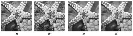
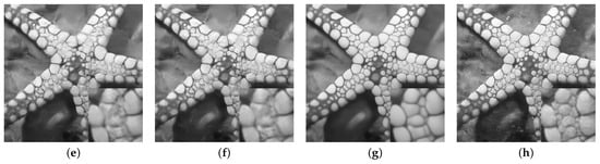
Figure 3. Denoising results of a gray noisy image from Set12 with $\sigma$ = 50. (a) Clean image, (b) Noisy image (14.90 dB/0.2869), (c) FFDNet (25.49 dB/0.7715), (d) DnCNN (25.60 dB/0.7715), (e) IRCNN (25.48 dB/0.7675), (f) NIFBGDNet (25.45 dB/0.7640), (g) DRUNet (26.49 dB/0.8013), (h) Ours (28.49 dB/0.8603).

For color Gaussian image denoising, the comparative denoising results are presented in Figure 4 and Figure 5. Upon closer examination, it was evident that our model effectively removed the majority of noise while preserving more detailed texture information, a feat not achieved by other methods. These visual comparisons further underscore the superior denoising performance of NGDCNet.

Figure 4. Denoising results of a color noisy image from Set5 with $\sigma$ = 25. (a) Clean image, (b) Noisy image (20.47 dB/0.6689), (c) FFDNet (31.04 dB/0.9379), (d) DnCNN (31.08 dB/0.9360), (e) IRCNN (30.95 dB/0.9342), (f) NIFBGDNet (30.84 dB/0.9348), (g) DRUNet (32.31 dB/0.9501), (h) Ours (32.87 dB/0.9614).

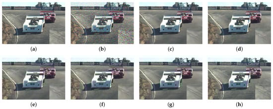
Figure 5. Denoising results of a color noisy image from CBSD68 with $\sigma$ = 50. (a) Clean image, (b) Noisy image (14.68 dB/0.3197), (c) FFDNet (28.29 dB/0.7577), (d) DnCNN (28.24 dB/0.7603), (e) IRCNN (28.19 dB/0.7614), (f) NIFBGDNet (27.96 dB/0.7507), (g) DRUNet (28.81 dB/0.7814), (h) Ours (30.27 dB/0.8541).

4.3.3. Ablation Experiments

In this section, the effects of DCB and NGB on NGDCNet’s performance were studied. Experiments were conducted on grayscale and color Gaussian images with noise levels of 15, 25, and 50. In order to evaluate the contributions of DCB and NGB, these components were individually removed from NGDCNet’s architecture for comparison. Specifically, for DCB, × means replacing the dynamic convolution in DCB with the standard convolution using the $3\times 3$ kernel. For NGB, × means to remove NGB and just do a normal skip connection.

Table 8 and Table 9 present the results of these ablation experiments for grayscale and color Gaussian images, respectively. The tables demonstrate that using either DCB or NGB alone results in improved performance for NGDCNet in both tasks. This suggests that DCB’s capacity to efficiently extract high-frequency information from features enhances the model’s performance in image denoising. NGB is effective in controlling the propagation of low-level feature information to higher levels, contributing to performance improvements in the denoising task.

Table 8. Study of ablation experiments of different components in gray scale image denoising on BSD68 [49] test set.

DCB	GB	15		25		50
		PSNR	SSIM	PSNR	SSIM	PSNR	SSIM
×	×	32.25	0.9138	30.23	0.8787	26.06	0.7507
✓	×	32.38	0.9154	30.49	0.8803	26.13	0.7772
×	✓	32.46	0.9163	30.78	0.8837	26.25	0.7827
✓	✓	32.60	0.9195	30.85	0.8869	28.28	0.8040

Table 9. Study of ablation experiments of different components in color scale image denoising on CBSD68 test set.

DCB	GB	15		25		50
		PSNR	SSIM	PSNR	SSIM	PSNR	SSIM
×	×	34.63	0.9520	32.84	0.9281	28.64	0.8337
✓	×	34.82	0.9522	32.85	0.9290	29.13	0.8392
×	✓	35.12	0.9539	33.20	0.9312	29.26	0.8654
✓	✓	35.34	0.9562	33.34	0.9339	29.85	0.8717

From the results in these tables, it can be observed that NGDCNet using DCB alone provides limited improvements in denoising performance because dynamic convolution is sensitive to noise [31]. In contrast, NGB can effectively filter information in the lower layers. When both DCB and NGB are combined, NGDCNet’s denoising performance is significantly enhanced. The last row in these tables shows the results of NGDCNet with combined DCB and NGB, demonstrating the effectiveness of this combined approach.

5. Conclusions

In this paper, we introduced a novel image denoising method, NGDCNet, which leverages a noise gating mechanism and dynamic convolution. NGDCNet is constructed through a collaboration of dynamic convolution blocks, noise gating blocks, and residual blocks. The dynamic convolution blocks employ stacked dynamic convolutions to capture high-frequency information within the features. The noise gating blocks effectively manage the flow of low-level feature information to higher layers, enhancing the model’s ability to process noise. Additionally, the residual blocks leverage residual operations to generate a denoised image.

Our proposed NGDCNet demonstrates impressive denoising performance, particularly in preserving image structure and fine details, even in high noise conditions. In future work, we aim to further evaluate NGDCNet in real image denoising tasks, extending its application to various practical scenarios. We believe that NGDCNet holds great promise for enhancing image quality and addressing real-world denoising challenges.

References

- Healey, G.E.; Kondepudy, R. Radiometric CCD camera calibration and noise estimation. IEEE Trans. Pattern Anal. Mach. Intell. 1994, 16, 267–276. [Google Scholar] [CrossRef]
- Diwakar, M.; Kumar, M. A review on CT image noise and its denoising. Biomed. Signal Process. Control 2018, 42, 73–88. [Google Scholar] [CrossRef]
- Gurrola-Ramos, J.; Dalmau, O.; Alarcón, T.E. A residual dense u-net neural network for image denoising. IEEE Access 2021, 9, 31742–31754. [Google Scholar] [CrossRef]
- Lee, J.S. Digital image enhancement and noise filtering by use of local statistics. IEEE Trans. Pattern Anal. Mach. Intell. 1980, PAMI-2, 165–168. [Google Scholar] [CrossRef] [PubMed]
- Kuan, D.T.; Sawchuk, A.A.; Strand, T.C.; Chavel, P. Adaptive noise smoothing filter for images with signal-dependent noise. IEEE Trans. Pattern Anal. Mach. Intell. 1985, PAMI-7, 165–177. [Google Scholar] [CrossRef] [PubMed]
- Zhang, B.; Allebach, J.P. Adaptive bilateral filter for sharpness enhancement and noise removal. IEEE Trans. Image Process. 2008, 17, 664–678. [Google Scholar] [CrossRef]
- Alkinani, M.H.; El-Sakka, M.R. Patch-based models and algorithms for image denoising: A comparative review between patch-based images denoising methods for additive noise reduction. EURASIP J. Image Video Process. 2017, 2017, 58. [Google Scholar] [CrossRef]
- Dabov, K.; Foi, A.; Katkovnik, V.; Egiazarian, K. Image denoising by sparse 3-D transform-domain collaborative filtering. IEEE Trans. Image Process. 2007, 16, 2080–2095. [Google Scholar] [CrossRef]
- Yang, D.; Sun, J. BM3D-Net: A convolutional neural network for transform-domain collaborative filtering. IEEE Signal Process. Lett. 2017, 25, 55–59. [Google Scholar] [CrossRef]
- Alrudaini, J.K.; Hayder, D.M.; Hamzah, A.K.; Ruhaina, A.A. Visual Perception Method for Medical Image De-noising. Malay. J. Med. Health Sci. 2022, 18, 40–44. [Google Scholar]
- Chambolle, A. An algorithm for total variation minimization and applications. J. Math. Imaging Vis. 2004, 20, 89–97. [Google Scholar]
- Perona, P.; Malik, J. Scale-space and edge detection using anisotropic diffusion. IEEE Trans. Pattern Anal. Mach. Intell. 1990, 12, 629–639. [Google Scholar] [CrossRef]
- Li, Q.; Jiang, L. A novel variable-separation method based on sparse and low rank representation for stochastic partial differential equations. SIAM J. Sci. Comput. 2017, 39, A2879–A2910. [Google Scholar] [CrossRef]
- Gu, S.; Zhang, L.; Zuo, W.; Feng, X. Weighted nuclear norm minimization with application to image denoising. In Proceedings of the IEEE Conference on Computer Vision and Pattern Recognition, Columbus, OH, USA, 23–28 June 2014; pp. 2862–2869. [Google Scholar]
- Lan, X.; Roth, S.; Huttenlocher, D.; Black, M.J. Efficient belief propagation with learned higher-order markov random fields. In Computer Vision, Proceedings of the ECCV 2006: 9th European Conference on Computer Vision, Graz, Austria, 7–13 May 2006; Proceedings, Part II 9; Springer: Berlin/Heidelberg, Germany, 2006; pp. 269–282. [Google Scholar]
- Li, P.; Liang, J.; Zhang, M.; Fan, W.; Yu, G. Joint image denoising with gradient direction and edge-preserving regularization. Pattern Recognit. 2022, 125, 108506. [Google Scholar] [CrossRef]
- Tian, C.; Fei, L.; Zheng, W.; Xu, Y.; Zuo, W.; Lin, C.W. Deep learning on image denoising: An overview. Neural Netw. 2020, 131, 251–275. [Google Scholar] [CrossRef]
- Zhang, K.; Zuo, W.; Gu, S.; Zhang, L. Learning deep CNN denoiser prior for image restoration. In Proceedings of the IEEE Conference on Computer Vision and Pattern Recognition, Honolulu, HI, USA, 21–26 July 2017; pp. 3929–3938. [Google Scholar]
- Zhang, K.; Zuo, W.; Chen, Y.; Meng, D.; Zhang, L. Beyond a gaussian denoiser: Residual learning of deep cnn for image denoising. IEEE Trans. Image Process. 2017, 26, 3142–3155. [Google Scholar] [CrossRef]
- Quan, Y.; Chen, Y.; Shao, Y.; Teng, H.; Xu, Y.; Ji, H. Image denoising using complex-valued deep CNN. Pattern Recognit. 2021, 111, 107639. [Google Scholar] [CrossRef]
- Tian, C.; Xu, Y.; Fei, L.; Wang, J.; Wen, J.; Luo, N. Enhanced CNN for image denoising. CAAI Trans. Intell. Technol. 2019, 4, 17–23. [Google Scholar] [CrossRef]
- He, K.; Zhang, X.; Ren, S.; Sun, J. Deep residual learning for image recognition. In Proceedings of the IEEE Conference on Computer Vision and Pattern Recognition, Las Vegas, NV, USA, 27–30 June 2016; pp. 770–778. [Google Scholar]
- Ioffe, S.; Szegedy, C. Batch normalization: Accelerating deep network training by reducing internal covariate shift. In Proceedings of the International Conference on Machine Learning, PMLR, Lille, France, 6–11 July 2015; pp. 448–456. [Google Scholar]
- Zhao, M.; Cao, G.; Huang, X.; Yang, L. Hybrid transformer-CNN for real image denoising. IEEE Signal Process. Lett. 2022, 29, 1252–1256. [Google Scholar] [CrossRef]
- Kumwilaisak, W.; Piriyatharawet, T.; Lasang, P.; Thatphithakkul, N. Image denoising with deep convolutional neural and multi-directional long short-term memory networks under Poisson noise environments. IEEE Access 2020, 8, 86998–87010. [Google Scholar] [CrossRef]
- Pang, T.; Zheng, H.; Quan, Y.; Ji, H. Recorrupted-to-recorrupted: Unsupervised deep learning for image denoising. In Proceedings of the IEEE/CVF Conference on Computer Vision and Pattern Recognition, Nashville, TN, USA, 20–25 June 2021; pp. 2043–2052. [Google Scholar]
- Zhang, Y.; Li, K.; Li, K.; Zhong, B.; Fu, Y. Residual non-local attention networks for image restoration. arXiv 2019, arXiv:1903.10082. [Google Scholar]
- Zou, X.; Xiao, F.; Yu, Z.; Li, Y.; Lee, Y.J. Delving deeper into anti-aliasing in convnets. Int. J. Comput. Vis. 2023, 131, 67–81. [Google Scholar] [CrossRef]
- Zhang, Y.; Li, K.; Li, K.; Sun, G.; Kong, Y.; Fu, Y. Accurate and fast image denoising via attention guided scaling. IEEE Trans. Image Process. 2021, 30, 6255–6265. [Google Scholar] [CrossRef] [PubMed]
- Chen, Y.; Dai, X.; Liu, M.; Chen, D.; Yuan, L.; Liu, Z. Dynamic convolution: Attention over convolution kernels. In Proceedings of the IEEE/CVF Conference on Computer Vision and Pattern Recognition, Seattle, WA, USA, 13–19 June 2020; pp. 11030–11039. [Google Scholar]
- Shen, H.; Zhao, Z.Q.; Zhang, W. Adaptive dynamic filtering network for image denoising. In Proceedings of the AAAI Conference on Artificial Intelligence, Washington, DC, USA, 7–14 February 2023; Volume 37, pp. 2227–2235. [Google Scholar]
- Ma, R.; Li, S.; Zhang, B.; Fang, L.; Li, Z. Flexible and generalized real photograph denoising exploiting dual meta attention. IEEE Trans. Cybern. 2022, 53, 6395–6407. [Google Scholar] [CrossRef] [PubMed]
- Ma, R.; Li, S.; Zhang, B.; Hu, H. Meta PID attention network for flexible and efficient real-world noisy image denoising. IEEE Trans. Image Process. 2022, 31, 2053–2066. [Google Scholar] [CrossRef] [PubMed]
- Ma, R.; Li, S.; Zhang, B.; Li, Z. Towards fast and robust real image denoising with attentive neural network and PID controller. IEEE Trans. Multimed. 2021, 24, 2366–2377. [Google Scholar] [CrossRef]
- Ma, R.; Hu, H.; Xing, S.; Li, Z. Efficient and fast real-world noisy image denoising by combining pyramid neural network and two-pathway unscented Kalman filter. IEEE Trans. Image Process. 2020, 29, 3927–3940. [Google Scholar] [CrossRef]
- Ma, R.; Li, S.; Zhang, B.; Li, Z. Generative adaptive convolutions for real-world noisy image denoising. In Proceedings of the AAAI Conference on Artificial Intelligence, Vancouver, BC, Canada, 20–27 February 2022; Volume 36, pp. 1935–1943. [Google Scholar]
- El Helou, M.; Süsstrunk, S. Blind universal Bayesian image denoising with Gaussian noise level learning. IEEE Trans. Image Process. 2020, 29, 4885–4897. [Google Scholar] [CrossRef]
- Yu, F.; Koltun, V. Multi-scale context aggregation by dilated convolutions. arXiv 2015, arXiv:1511.07122. [Google Scholar]
- Zhang, K.; Zuo, W.; Zhang, L. FFDNet: Toward a fast and flexible solution for CNN-based image denoising. IEEE Trans. Image Process. 2018, 27, 4608–4622. [Google Scholar] [CrossRef]
- Lan, R.; Zou, H.; Pang, C.; Zhong, Y.; Liu, Z.; Luo, X. Image denoising via deep residual convolutional neural networks. Signal Image Video Process. 2021, 15, 1–8. [Google Scholar] [CrossRef]
- Xu, M.; Xie, X. NFCNN: Toward a noise fusion convolutional neural network for image denoising. Signal Image and Video Process. 2022, 16, 175–183. [Google Scholar] [CrossRef]
- Ren, C.; He, X.; Wang, C.; Zhao, Z. Adaptive consistency prior based deep network for image denoising. In Proceedings of the IEEE/CVF Conference on Computer Vision and Pattern Recognition, Nashville, TN, USA, 20–25 June 2021; pp. 8596–8606. [Google Scholar]
- Li, B.; Liu, X.; Hu, P.; Wu, Z.; Lv, J.; Peng, X. All-in-one image restoration for unknown corruption. In Proceedings of the IEEE/CVF Conference on Computer Vision and Pattern Recognition, New Orleans, LA, USA, 18–24 June 2022; pp. 17452–17462. [Google Scholar]
- Zhang, K.; Li, Y.; Zuo, W.; Zhang, L.; Van Gool, L.; Timofte, R. Plug-and-play image restoration with deep denoiser prior. IEEE Trans. Pattern Anal. Mach. Intell. 2021, 44, 6360–6376. [Google Scholar] [CrossRef] [PubMed]
- Zhang, Q.; Xiao, J.; Tian, C.; Chun-Wei Lin, J.; Zhang, S. A robust deformed convolutional neural network (CNN) for image denoising. CAAI Trans. Intell. Technol. 2023, 8, 331–342. [Google Scholar] [CrossRef]
- Tian, C.; Zheng, M.; Zuo, W.; Zhang, B.; Zhang, Y.; Zhang, D. Multi-stage image denoising with the wavelet transform. Pattern Recognit. 2023, 134, 109050. [Google Scholar] [CrossRef]
- Yu, J.; Lin, Z.; Yang, J.; Shen, X.; Lu, X.; Huang, T.S. Free-form image inpainting with gated convolution. In Proceedings of the IEEE/CVF International Conference on Computer Vision, Long Beach, CA, USA, 15–20 June 2019; pp. 4471–4480. [Google Scholar]
- Chang, Y.L.; Liu, Z.Y.; Lee, K.Y.; Hsu, W. Free-form video inpainting with 3d gated convolution and temporal patchgan. In Proceedings of the IEEE/CVF International Conference on Computer Vision, Long Beach, CA, USA, 15–20 June 2019; pp. 9066–9075. [Google Scholar]
- Roth, S.; Black, M.J. Fields of experts: A framework for learning image priors. In Proceedings of the 2005 IEEE Computer Society Conference on Computer Vision and Pattern Recognition (CVPR’05), San Diego, CA, USA, 20–25 June 2005; Volume 2, pp. 860–867. [Google Scholar]
- Mairal, J.; Bach, F.; Ponce, J.; Sapiro, G.; Zisserman, A. Non-local sparse models for image restoration. In Proceedings of the 2009 IEEE 12th International Conference on Computer Vision, Kyoto, Japan, 29 September–2 October 2009; pp. 2272–2279. [Google Scholar]
- Hore, A.; Ziou, D. Image quality metrics: PSNR vs. SSIM. In Proceedings of the 2010 20th International Conference on Pattern Recognition, Istanbul, Turkey, 23–26 August 2010; pp. 2366–2369. [Google Scholar]
- Wang, Z.; Bovik, A.C.; Sheikh, H.R.; Simoncelli, E.P. Image quality assessment: From error visibility to structural similarity. IEEE Trans. Image Process. 2004, 13, 600–612. [Google Scholar] [CrossRef] [PubMed]
- Bevilacqua, M.; Roumy, A.; Guillemot, C.; Alberi-Morel, M.L. Low-complexity single-image super-resolution based on nonnegative neighbor embedding. In Proceedings of the 23rd British Machine Vision Conference (BMVC), Surrey, UK, 3–7 September 2012. [Google Scholar]
- Ephraim, Y.; Malah, D. Speech enhancement using a minimum-mean square error short-time spectral amplitude estimator. IEEE Trans. Acoust. Speech Signal Process. 1984, 32, 1109–1121. [Google Scholar] [CrossRef]
- Ding, K.; Ma, K.; Wang, S.; Simoncelli, E.P. Image quality assessment: Unifying structure and texture similarity. IEEE Trans. Pattern Anal. Mach. Intell. 2020, 44, 2567–2581. [Google Scholar] [CrossRef]
- Devalla, S.K.; Renukanand, P.K.; Sreedhar, B.K.; Subramanian, G.; Zhang, L.; Perera, S.; Mari, J.M.; Chin, K.S.; Tun, T.A.; Strouthidis, N.G.; et al. DRUNET: A dilated-residual U-Net deep learning network to segment optic nerve head tissues in optical coherence tomography images. Biomed. Opt. Express 2018, 9, 3244–3265. [Google Scholar] [CrossRef]
- Thakur, R.K.; Maji, S.K. Multi scale pixel attention and feature extraction based neural network for image denoising. Pattern Recognit. 2023, 141, 109603. [Google Scholar] [CrossRef]
Disclaimer/Publisher’s Note: The statements, opinions and data contained in all publications are solely those of the individual author(s) and contributor(s) and not of MDPI and/or the editor(s). MDPI and/or the editor(s) disclaim responsibility for any injury to people or property resulting from any ideas, methods, instructions or products referred to in the content. |
© 2023 by the authors. Licensee MDPI, Basel, Switzerland. This article is an open access article distributed under the terms and conditions of the Creative Commons Attribution (CC BY) license (https://creativecommons.org/licenses/by/4.0/).