LiDAR Localization by Removing Moveable Objects

Abstract

In this study, we propose reliable Light Detection and Ranging (LiDAR) mapping and localization via the removal of moveable objects, which can cause noise for autonomous driving vehicles based on the Normal Distributions Transform (NDT). LiDAR measures the distances to objects such as parked and moving cars and objects on the road, calculating the time of flight required for the sensor’s beam to reflect off an object and return to the system. The proposed localization system uses LiDAR to implement mapping and matching for the surroundings of an autonomous vehicle. This localization is applied to an autonomous vehicle, a mid-size Sports Utility Vehicle (SUV) that has a 64-channel Velodyne sensor, detecting moveable objects via modified DeepLabV3 and semantic segmentation. LiDAR and vision sensors are popular perception sensors, but vision sensors have a weakness that does not allow for an object to be detected accurately under special circumstances, such as at night or when there is a backlight in daylight. Even if LiDAR is more expensive than other detecting sensors, LiDAR can more reliably and accurately sense an object with the right depth because a LiDAR sensor estimates an object’s distance using the time of flight required for the LiDAR sensor’s beam to detect the object and return to the system. The cost of a LiDAR product will decrease dramatically in the case of skyrocketing demand for LiDAR in the industrial areas of autonomous vehicles, humanoid robots, service robots, and unmanned drones. As a result, this study develops a precise application of LiDAR localization for a mid-size SUV, which gives the best performance with respect to acquiring an object’s information and contributing to the appropriate, timely control of the mid-size SUV. We suggest mapping and localization using only LiDAR, without support from any other sensors, such as a Global Positioning System (GPS) or an Inertial Measurement Unit (IMU) sensor; using only a LiDAR sensor will be beneficial for cost competitiveness and reliability. With the powerful modified DeepLabV3, which is faster and more accurate, we identify and remove a moveable object through semantic segmentation. The improvement rate of the mapping and matching performance of our proposed NDT, by removing the moveable objects, was approximately 12% in terms of the Root-Mean-Square Error (RMSE) for the first fifth of the test course, where there were fewer parked cars and more moving cars.

1. Introduction

A GPS sensor error is shown in Figure 1; errors occur because GPS signals from satellites can be blocked by many tall buildings and refracted by the buildings’ glass. The solid red line shows the GPS sensor’s latitude and longitude on a satellite map; the line is disconnected in spite of a closed-loop course. The experimental vehicle was an autonomous mid-size SUV that was driven by a human driver, and the yellow-highlighted cells indicate both the real starting point and the real end point. In the blue circle, a GPS error was detected; the GPS signal diverged, and the red line was not closed. My personal experience was that when using Google Maps on my mobile phone, the GPS location froze and oscillated in a new city, which has the tallest buildings in the world. In these areas, in the centers of large cities that have taller buildings, GPS sensor errors can occur, and we need to correct the GPS sensor or develop another reliable system. Figure 1 shows the rationale for why we use LiDAR NDT mapping and location in the case of a city with taller buildings and underground parking lots.

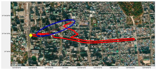
Figure 1. Global Positioning System (GPS) error at Seoul City Hall, Seoul, Republic of Korea.

A GPS error analysis is important for understanding how a GPS works and the magnitude of the prediction error. The satellite positioning system corrects incoming clock errors and other effects, but there are some remaining uncorrected errors. A GPS receiver’s position is calculated based on data received from a satellite. A GPS receiver requires the current time, the satellite’s position, and the measurement delay of the received signal. Location accuracy depends primarily on the satellite’s position and signal delay.

In the case of a general road environment with more moveable objects, there are impacts on the localization performance caused by large differences between mapping data and LiDAR sensing data. In order to solve the performance decline problem, we removed the moveable objects via the application of a deep-learning-based semantic segmentation method. As a result, an improvement in the test result is confirmed for mapping and map matching after removing moveable objects in the original LiDAR sensor data. In order to remove the moveable objects, we needed to identify each object’s classification through semantic segmentation, using modified DeepLabV3 (which was developed based on a Python deep learning process) and Velodyne LiDAR learning data, and extract the frozen parameters first. The moveable objects identified using semantic segmentation and frozen parameters were removed using the Robot Operating System (ROS), and the performance was improved compared to the previous NDT logic by removing noise, such as moveable objects, once the NDT program was running.

2. Related Works

Important and meaningful data are acquired from various sensors, which are LiDAR, camera, and IMU sensors, through the communication of multiple autonomous vehicles. We can obtain important information, such as the vehicle’s identification number, current position, moving speed, and informed orientation. From deep learning post-processing, we can extract useful information for object identification and detection and the filter noise level and remove outliers. The refined generated High-Definition (HD) map is to be used for multiple purposes in transportation research and to study autonomous vehicles [1].

Due to environmental transitions, such as the seasonal change from summer to winter, the performance for mapping and map matching is decreased, and this creates an accuracy problem. The changing environment has a significant impact on the localization accuracy due to uncertain noise. The inertial dead reckoning compensates LiDAR NDT mapping and localization. Even though autonomous vehicles are tested in two seasons, summer and winter, which have completely different environments, the accuracy merit of integration with inertial dead reckoning has been determined, with a good result for the reduction of computation complexity [2].

Autonomous vehicles require a lot of sensors to secure safety, which is a very important factor for increasing the autonomous vehicle economy. In terms of securing both safety and cost effectiveness, we propose only LiDAR mapping and map localization by confirming the safety factor. The other GPS sensor is only used for ground truth in this paper.

GPS errors happen due to time delays and unidentified reasons, and it is difficult to localize an autonomous vehicle using only GPS. Therefore, sensor fusion is required to overcome the drawbacks of GPS in terms of the hardware perspective, and we need to apply a fast and reliable filter, such as a Kalman filter or the Unscented Kalman Filter (UKF), in terms of the software perspective [3]. Therefore, we introduce LiDAR localization by removing moveable objects in the NDT in specific areas where GPS does not operate in an appropriate amount of time and in special situations in cities where a lot of moving objects, such as vehicles and bicycles, are regarded as noise. The performance is expected to be improved in cities compared to rural areas.

From the perspective of processing speed, we use the NDT for a faster processing speed rather than the Iterative Closest Point (ICP), which has a heavy calculation process, but the NDT program is updated and changed for various environmental situations. In the NDT, each cell is split from the LiDAR scan data, and the normal distribution character of each cell is matched with new input data based on the reference cell. The proposed NDT is improved in the case of the removal of moveable objects compared to the original NDT.

Laser scan mapping and localization based on the NDT are essential for a moveable robot system, and they are popular due to their higher reliability and accuracy. The designed robot was tested for around 80 m in the lab and out of the lab without using odometry, and it showed the ability to build a reliable map [4]. The eigen valve modification improves the NDT high-resolution grid map. The NDT is efficient for a large grid, but it is difficult to build a small grid map due to errors for small objects around walls, the surfaces of walls, and the edges of objects. Through the modified eigen valve, we eliminate these errors and build NDT scan matching properly [5]. Simultaneous Localization and Mapping (SLAM) consists of front-process odometry and back-process optimization based on the LiDAR NDT. It adjusts the weighted factor in each cell according to the range’s value and the surface’s characteristics, and an updated cost function is constructed, which give the values for both accuracy and efficiency [6].

There are a lot of methods to identify the objects in an image, categorized into vehicles, people, riders, and so on. The representative methods are semantic segmentation, instance segmentation, and panoptic segmentation, which combines both semantic segmentation and instance segmentation. Instance segmentation is divided into two groups; one is the foreground image, and the other is the background image. It extracts semantic segmentation only from the foreground, which contains important countable objects. In this paper, we use the sematic segmentation method and the modified DeepLabV3, which has a fast processing speed and better accuracy than other methods when identifying moveable objects and removing them.

Image identification is one of the key components of cognitive systems in autonomous vehicles, such as self-driving cars or delivery robots. An autonomous vehicle’s cognitive system acquires information from LiDAR, cameras, and radar sensors. Scene understanding includes object detection and segmentation [7]. Object detection detects the objects’ classifications and locations in the images. Segmentation obtains object classification information in each pixel and is split into the instance, semantic, and panoptic segmentations. Instance segmentation includes the classification information of important objects and segmented information. Semantic segmentation contains the classification information of all pixels in the scene. Panoptic segmentation obtains synthesized information from instance segmentation and semantic segmentation [8]. Scene understanding is essential for the environmental awareness of autonomous vehicles. Scene comprehension started with the early methods of finding and analyzing features and has been continuously developed through the application of deep learning [9]. The goal of scene recognition in computer vision is to recognize all elements of images. Images are divided into the foreground and background. The background, which is uncountable, and the foreground object, which is countable, are considered important objects. An object detection algorithm, such as You Only Look Once (YOLO) proposed by Redmon, is used to find these important objects. YOLO has been studied up to V5 due to its consistent popularity [10]. Methods for detecting objects in pixel units in an image are separated into instance, semantic, and panoptic segmentations. Mask r-cnn, a representative study of instance segmentation, added the Mask branch to the Region Proposal Network (RPM) structure proposed by Fast r-cnn [11]. Instance segmentation segments only the important objects. Semantic segmentation segments the entire scene. DeepLab was proposed [12]. Panoptic segmentation aims for a more complete scene understanding by including the results of both methods. A Feature Pyramid Network (FPN) was used for panoptic segmentation, and a structure was proposed to predict the foreground and background by dividing them into an instance segmentation head and a semantic segmentation head, combining the prediction results in the panoptic segmentation head [13]. A system based on LiDAR uses a single network for object detection and classification. The DeepLabV3+ network from a previous study was modified to be appropriate for the LiDAR data used in this study. The system provides object detection and classification data for LiDAR data [14]. We contribute state-of-the-art semantic segmentation for LIDAR and give this categorized information to the vehicle. This approach performs semantic segmentation using LiDAR point clouds [15].

In autonomous vehicles, there are three steps for them to move. The first is perception, the second is to decide where to go, and the last is to control the steering and handling, operating well. Perception is very important to control the vehicle, similar to the human eye. Humans cannot go anywhere without eyes, and there is a similar situation for vehicles. In particular, we call LiDAR the center of an autonomous vehicle’s detection of objects [16]. LiDAR, like the human eye, is used to localize autonomous vehicles and move them to the locations where they want to go, controlling the steering and braking systems [17].

There are three kinds of localization methods. The first is vison localization, which has had a problem with accuracy until now, and the second is GPS localization, which has a disadvantage due to the inability to receive GPS signals in specific areas near the tallest buildings and in tunnels. The third is LiDAR localization to overcome the disadvantage of GPS localization. However, current LiDAR localization could cause some errors in situations with more moving objects, generating noise. Therefore, we suggest the updated LiDAR localization by removing possible noise and moveable objects using the modified DeepLabV3.

A novel 3D LiDAR localization with curb detection was proposed, but autonomous vehicles failed to be localized once the curb detection was blocked by other objects [18]. Reliable LiDAR localization is a fundamental factor in the autonomous vehicle industry. We implemented a surfel map using Velodyne LiDAR rotating source data and estimated the pose by computing an optimization through a comparison between the current scan and the next scan in the surfel map [19]. We made a spherical projection from the LiDAR source data, and semantic segmentation information was extracted from a convolutional neural network. The calculated semantic segmentation with labeled surfels allowed us to filter the moving objects reliably and improve the scan matching to clear the noise. The experiment was implemented using a highway sequence from the Karlsruhe Institute of Technology and Toyota Technological Institute (KITTI) dataset, and moving cars gave merit to our sematic segmentation Simultaneous Localization and Mapping (SLAM) [20]. With 3D LiDAR, we measured and analyzed the special behavior of professional caregivers helping patients and testing in a hospital. An observer carried the attached 3D LiDAR system on his back and followed them. A 3D LiDAR map was built, and the system simultaneously detected and tracked the position while calculating the sensor’s position [21]. An HD map is required to localize autonomous vehicles, and localization performance could decline without an HD map. On the other hand, an HD map requires an extremely large capacity, and the large storage space will impact real-time computation and the actual performance. A lower-resolution map could make the computation speed faster, but it would cause a performance problem where the localization would not match properly. As a result, we can obtain accuracy and efficiency using the Vehicle to Infrastructure (V2I)-based LiDAR localization method [22].

Dynamic objects in a laser scan degrade the localization accuracy, and a novel and robust method to remove dynamic objects is proposed. The speed of building an occupancy map is increased using object detection and the voxel traversal process [23]. The robustness of a LiDAR lateral localization system was improved, and its application with the fusion of a camera was tested in central Oxford. This system can leverage a method to detect an occluded road boundary and improve LiDAR lateral localization compared to a GPS initialization of the lateral localization [24]. Dynamic objects degrade the map’s quality performance, and the proposed baseline is to remove the dynamic objects for loop closure detection and to give a superior performance compared to the conventional process, using LiDAR Iris on the pre-processed data [25]. In order to build a clean map, it is necessary to remove the dynamic objects, and ground segmentation is used to separate dynamic objects and static road backgrounds. A static map generation result shows a perfect performance when generating a clean map [26].

The Interacting Multiple Model (IMM) program is used to track and measure an object’s velocity, assuming that it is linear. However, we needed to modify the IMM algorithm in the case of a nonlinear model to track objects accurately and properly. We replaced the Extended Kalman Filter (EKF) with the UKF for more efficient performance due to the nonlinear environment, and the Joint Probabilistic Data Association (JPDA) was integrated with the IMM-UKF algorithm in order to solve the data association problem [27]. We plan to use the JPDA-IMM-UKF algorithm in future work to filter moving objects, and we expect further performance improvements.

3. Materials

We analyzed NDT mapping and localization through an experiment to acquire LiDAR cloud data and GPS data using the remodeled autonomous mid-size SUV in Figure 2.

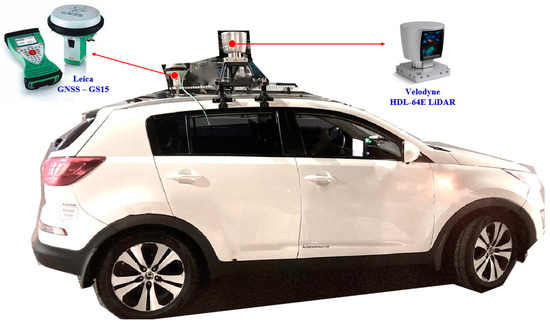
Figure 2. The platform of the remodeled mid-size SUV.

Figure 3 shows a diagram of the LiDAR detection range, and the LiDAR sensor detection range was about 50 m, which is highlighted in the blue circle.

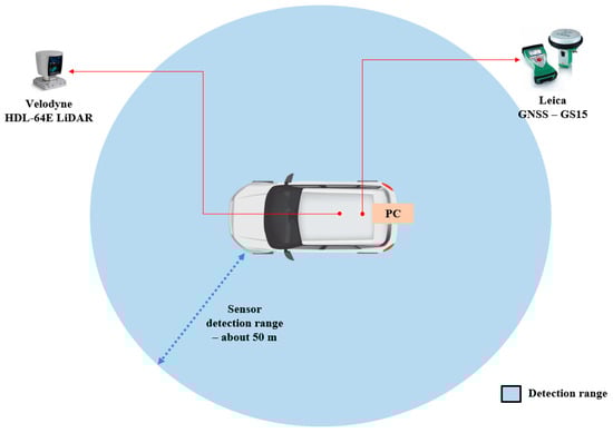
Figure 3. Diagram of LiDAR detection range.

The detailed specifications of the experimental hardware of the sensors and equipment are described in Table 1. There were two sensors attached to the test vehicle. One sensor was a 64-channel Velodyne LiDAR on the top of the vehicle, and the other sensor was a Leica GS15 GPS sensor on the top of the vehicle. The test’s desktop PC used the Melodic Robot Operation System (ROS) in Ubuntu 18.04 LTS. Real-time data were acquired from the LiDAR and GPS by the ROS via a communication method in the master management module. The LiDAR and GPS topics were subscribed from the master PC, which was installed in the autonomous vehicle in an ROS environment. The ROS contains a powerful software library and helps users to communicate sensor data well when building robot applications. The ROS is open-source from the drivers to the accurate and reliable algorithms for robot developers and autonomous vehicle engineers.

Table 1. Experimental hardware specifications.

Item	Manufacturer	Model	Specification	Remarks
Sensor	Velodyne (San Jose, CA, USA)	HDL-64E	64 channels Vertical FOV: 26.9 degrees Vertical resolution: 0.4 degrees Horizontal resolution: 0.08–0.35 degrees	Top
PC		Desktop	Ubuntu 18.04 ROS Melodic Intel i9-9940X CPU @ 3.30 GHz Nvidia RTX-2080Ti×3 pieces RAM: 128 GB
Vehicle	Kia (Seoul, Republic of Korea)	Sportage	Size: 4400 × 1855 × 1635 mm Weight: 1548 kg Displacement: 1955cc Maximum power: 184 HP Maximum torque: 41.0 kg×m Steering angle: −520°~ +540° Steering speed: 112.3 deg/s Steering ratio: 16/4:1
GPS	Leica (Wetzlar, Germany)	Leica GS15	Weight: 1.34 kg Error range: 8 mm horizontal, 15 mm vertical Number of satellites: up to 60 satellites Reaction time: under 1 s	Top

4. Method

This study aimed to develop exact and on-time mapping and localization with 64-channel Velodyne LiDAR, removing moveable objects, such as vehicles and bicycles. Raw LiDAR data were detected at a frequency of 10 Hz. Figure 4 shows the concept of LiDAR mapping and localization by removing moveable objects. The proposed mapping and localization consists of two categories. One is moveable object elimination, and the other is NDT processing. Moveable object elimination is a key factor in our paper. Moveable object elimination means that we identify moveable objects using the semantic segmentation method and DeepLabV3 and remove the moveable objects in the ROS.

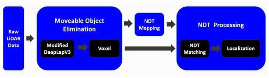
Figure 4. The concept of LiDAR mapping and localization by removing moveable objects.

We failed NDT mapping first due to a delayed process, which required heavier optimization and transformation calculation. Therefore, we applied a voxel filter in the proposed system. NDT mapping was successful with the voxel filter (filter size: 1 m), as shown in the right picture of Figure 5.

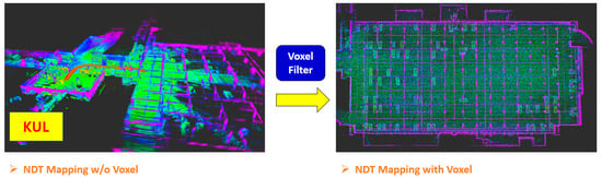
Figure 5. NDT mapping comparison with and without voxel filter.

Assuming that there are no rotations, the transformation matrix represents only the translation movement to point P and its translation matrix. This equation is only described for joint-position linear movement, not rotated movement. Based on a Cartesian coordinate system, the translation matrix describes the linear slide cylinder and is used for both the forward and inverse kinematic equations for the position of each robot joint. The P vector length is a key factor when the scale factor is one, and the matrix is described as a 3 × 4 matrix in the case of no scale factors, which is generally not the case [28].

$$T_{cart}=\left[\begin{array}{c}\\ 000P_x\\ 010P_y\\ 001P_z\\ 0001\\ \end{array}\right]$$

(1)

Three rotations normally exist in an autonomous vehicle based on the gravity center reference frame. The first rotation is ${\varnothing }_a$, which we generally call roll, and the reference axis is the vehicle heading axis. The second rotation is ${\varnothing }_o$, which we generally call pitch, and the reference axis is the lateral axis. The third rotation is ${\varnothing }_n$, which we generally call yaw, and the reference axis is the vertical axis from the ground to the sky. The RPY orientation consists of three kinds of roll, pitch, and yaw, totally integrating and describing the three rotations in sequence. The symbol ‘S’ is expressed for sine, the symbol ‘C’ is expressed for cosine, and the total combined matrix integrates three rotations, which has been described [28].

$$\begin{gathered} RPY\left({\varnothing }_{a,}{\varnothing }_{o,}{\varnothing }_n\right)=Rot\left(a,{\varnothing }_a\right)\ast Rot\left(o,{\varnothing }_o\right)\ast Rot\left(n,{\varnothing }_n\right)= \\ \left[\begin{array}{c}\\ C{ø}_a{\mathrm{C}ø}_{o}C{ø}_a{\mathrm{S}ø}_{o}S{ø}_n-S{ø}_a{\mathrm{C}ø}_{n}C{ø}_a{\mathrm{S}ø}_{o}C{ø}_n+S{ø}_a{\mathrm{C}ø}_{n}0\\ S{ø}_a{\mathrm{C}ø}_{o}S{ø}_a{\mathrm{S}ø}_{o}S{ø}_n+C{ø}_a{\mathrm{C}ø}_{n}S{ø}_a{\mathrm{S}ø}_{o}C{ø}_n-C{ø}_a{\mathrm{S}ø}_{n}0\\ {-\mathrm{S}ø}_{o}C{ø}_o{\mathrm{S}ø}_{n}C{ø}_o{\mathrm{C}ø}_{n}0\\ 0001\\ \end{array}\right] \end{gathered}$$

(2)

Once we express the coordinates of the $i_{th}$ points in the grid as ‘$x_i$’, the distribution mean ($\mu$) and distribution covariance ($\mathsf{\Sigma }$) are expressed in the following equation.

$$\mu =\frac{1}{n}{\displaystyle \sum }_{i=1}^n{x}_i$$

(3)

$$\mathsf{\Sigma }=\frac{1}{n}{\displaystyle \sum }_{i=1}^n\left(x_i-\mu \right){\left(x_i-\mu \right)}^T$$

(4)

The normal distribution probability ($p\left(x\right)$) is expressed in the following equation.

$$p\left(x\right)~e^{-\frac{{\left(x-\mu \right)}^T{\mathsf{\Sigma }}^{-1}\left(x-\mu \right)}{2}}$$

(5)

In terms of two dimensions, the spatial mapping (T) for the coordinate transformation is expressed in the following equation.

$$\begin{gathered} \mathbf{T}:\left(\begin{array}{c}{x}^{\prime }\\ y^{\prime }\end{array}\right)=\left(\begin{array}{cc}\cos \varphi & -\sin \varphi \\ \sin \varphi & \cos \varphi \end{array}\right)\left(\begin{array}{c}x\\ y\end{array}\right)+\left(\begin{array}{c}{t}_x\\ t_y\end{array}\right) \\ =\left(\begin{array}{c}x\cos \varphi -y\sin \varphi +t_x\\ x\sin \varphi +y\cos \varphi +t_y\end{array}\right) \end{gathered}$$

(6)

$\mathrm{where}{t}_x$ and $t_y$ express the translation movement, and $\varphi$ describes the rotation movement of two scan data in a sequence in terms of the time perspective. The mapping implementation is completed between the first scan datapoint and the next scan datapoint, making a calculation of the normal distribution and completing the optimization using the score equation (Equation (7)). $x_i$ describes a sample of the scanned LiDAR points, and $x_i^{\prime }$ indicates that $x_i$ is sorted by the parameters in $\mathrm{P}$. The equation is $x_i^{\prime }=T\left(x_i,\mathrm{P}\right)$. The $\mathrm{P}$ score describes the matching optimization value in the following equation.

$$\mathrm{Score}\left(\mathrm{P}\right)={\displaystyle \sum }_{i=1}^n{e}^{-\frac{{\left(x_i^{\prime }-{\mu }_i\right)}^T{\mathsf{\Sigma }}^{-1}\left(x_i^{\prime }-{\mu }_i\right)}{2}}$$

(7)

For mapping optimization, we need to determine the optimal parameters (P) to minimize the function ($f$) using the Newton algorithm. The parameters (P) minimize the function using the gradient ($\mathit{g}$) of the function ($f$) and the Hessian matrix (H). $s$ is described as follows.

$$H\Delta \mathrm{p}=-\mathit{g}$$

(8)

$$g_i=\frac{\partial f}{\partial p_i}$$

(9)

$$H_{ij}=\frac{\partial f}{\partial p_i\partial p_j}$$

(10)

$$\mu =x_i^{\prime }-{\mu }_i, s=-e^{\frac{-{\mu }^T{\mathsf{\Sigma }}^{-1}\mu }{2}}$$

(11)

In terms of $P_i$, the partial derivative of $\mu$ can be described by $x_i^{\prime }$, and the score function gradient is completed using Equation (11) as a summand. Therefore, the partial derivative of $\mu$ is estimated as the Jacobian matrix ($J_T$) of T. The Hessian matrix is estimated using the score function partial derivatives in terms of every parameter.

$${\tilde{g}}_i=-\frac{\partial s}{\partial p_i}=-\frac{\partial s\partial \mu }{\partial \mu \partial p_i}={\mu }^T{\mathsf{\Sigma }}^{-1}\frac{\partial \mu }{\partial p_i}{e}^{\frac{-{\mu }^T{\mathsf{\Sigma }}^{-1}\mu }{2}}$$

(12)

$$J_T=\left(\begin{array}{ccc}1& 0& -x\sin \varphi -y\cos \varphi \\ 1& 1& x\cos \varphi -y\sin \varphi \end{array}\right)$$

(13)

The Hessian matrix (H) is described in Equation (14), and the second partial derivative of $\mu$ is described using Equation (15).

$${\tilde{H}}_{ij}=-\frac{\partial s}{\partial p_i\partial p_j}=-e^{\frac{-{\mu }^T{\mathsf{\Sigma }}^{-1}\mu }{2}}\left(\left(-{\mu }^T{\mathsf{\Sigma }}^{-1}\frac{\partial \mu }{\partial p_i}\right)\left(-{\mu }^T{\mathsf{\Sigma }}^{-1}\frac{\partial \mu }{\partial p_j}\right)+\left(-{\mu }^T{\mathsf{\Sigma }}^{-1}\frac{{\partial }^2\mu }{\partial p_i\partial p_j}\right)+\left(-\frac{\partial {\mu }^T}{\partial p_j}{\mathsf{\Sigma }}^{-1}\frac{\partial \mu }{\partial p_i}\right)\right)$$

(14)

$$\frac{{\partial }^2\mu }{\partial p_i\partial p_j}=\left\{\begin{array}{c}\left(\begin{array}{c}-x\cos \varphi +y\sin \varphi \\ -x\sin \varphi -y\cos \varphi \end{array}\right), i=j=3\\ \left(\begin{array}{c}0\\ 0\end{array}\right) , otherwise\end{array}\right\}$$

(15)

The Hessian matrix is used for NDT function optimization and position estimation. Using the Hessian matrix, we calculate the derivatives of the NDT function and make a correction for position estimation. The Hessian matrix gives curvature information and the NDT function’s second-order derivative. It optimizes the function efficiently and refines the forecasted position [22].

The spherical coordinate system in Figure 6 can be used to convert to the image coordinate system, as shown in Equation (16).

$$\left(\begin{array}{c}u\\ v\end{array}\right)=\left(\begin{array}{c}1/2\left[1-\arctan \left(y,x\right){\pi }^{-1}\right]W\\ \left[1-\left(\arcsin \left(z{r}^{-1}\right)+f_{up}\right)f^{-1}\right]H\end{array}\right)$$

(16)

$\mathrm{where}H$ is the height of an image, and $W$ is the width of an image, while x, y, and z represent the LiDAR data. $f$ is the Field of View (FOV) of the sensor, as shown in Equation (17).

$$f=f_{up}+f_{down}$$

(17)

where $r$ is the distance from the sensor to the point, as shown in Equation (18).

$$r=\sqrt{x^2+y^2+z^2}$$

(18)

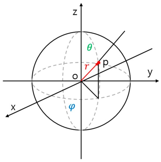
Figure 6. Spherical coordinates.

The LiDAR data and $r$ are projected onto a transformed coordinate system to generate an image [14]. The converted data are shown in Figure 7. The moveable objects, such as vehicles, were removed from the lower picture, and the vehicles are categorized in blue. The raw LiDAR data were changed for the lower picture, removing the moveable objects such as vehicles, categorized in blue through semantic segmentation.

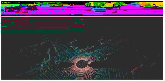
Figure 7. Point cloud and LiDAR data projected by removing objects.

5. Experiments and Results

We drove a mid-size SUV in a closed loop near the National Assembly. The red circle indicates that we started and finished the journey in the same position. Both absolute coordinate latitude and longitude GPS data are described in Figure 8. The experiment’s resulting data are the extracted averages from four closed-loop journeys in the blue triangle line around the National Assembly in the Republic of Korea.

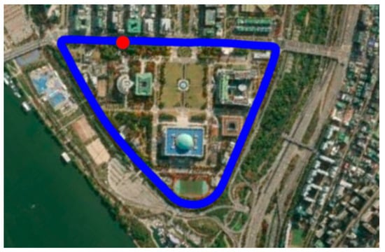
Figure 8. Latitude and longitude GPS data near National Assembly, Seoul, Republic of Korea.

We mapped the closed-loop course using the NDT program, and the calculated trajectory is shown in Figure 9. Both Figure 10 and Figure 11 show similar trajectories for the test line, and they have triangular shapes.

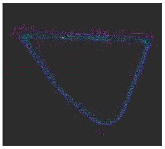
Figure 9. NDT map near National Assembly, Seoul, Republic of Korea.

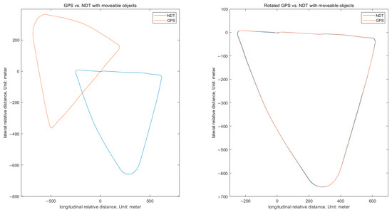
Figure 10. Comparison between NDT matching with moveable objects and GT (GPS).

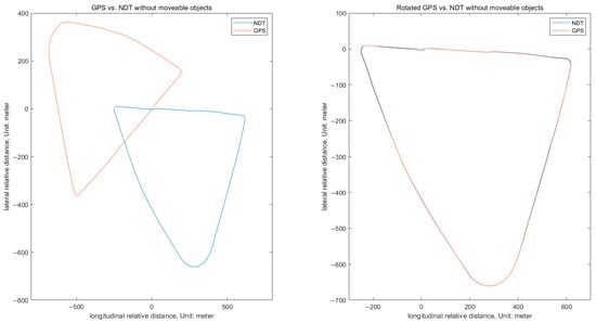
Figure 11. Comparison between NDT matching by removing moveable objects and GPS.

The ground truth is the red solid line (GPS data), which is based on the global absolute coordinates for latitude and longitude, and the blue solid line is NDT matching with moveable vehicles. However, NDT-matching coordinates are relative, and the origin is almost zero. In order to match the GPS absolute coordinates with the NDT coordinates, we moved the first GPS point to the origin (x = 0, y = 0) using the Equation (1) translation transformation matrix through the parallel movement in the left picture in Figure 10. However, the two trajectories were not yet comparable to determine the Root-Mean-Square Error (RMSE), and the trajectory needed to be rotated. First, we determined each unit vector between the start point and the next point to calculate the rotation angle between the GPS trajectory and the NDT-matching trajectory in the right picture of Figure 9 using Equation (2) (RPY orientation).

Figure 11 shows a performance comparison between GPS data and NDT matching by removing moveable objects in converted raw LiDAR data using the modified DeepLabV3.

As a result, we compared the RMSE between NDT matching with moveable objects and NDT matching removing moveable objects, as shown in Table 2. The RMSE of all trajectories of NDT matching with moveable objects is 0.9870, and the RMSE of all trajectories of NDT matching without moveable objects is 1.1623. The performance of our proposed NDT was inferior to normal NDT matching because one lane was full of parked cars, which are a good feature for NDT mapping and matching, after the first fifth of the course in the test area.

Table 2. Comparison of RMSE between proposed and previous NDTs.

Model	RMSE in the First 1/5 of the Course	RMSE in the Entire Course	Moveable	GT
Proposed NDT	0.1752	1.1623	Excluded	GPS
Previous NDT	0.1970	0.9870	Included	GPS

We operated the SUV four times by configuring the closed loop with the same starting and stopping positions. The data described in Table 3 are the RMSE of each iteration for the proposed NDT, which was run four times. Figure 12 shows the same position for every iteration with different surroundings, such as vehicles.

Table 3. RMSE for every iteration of proposed NDT.

Model	RMSE in the First 1/5 of the Course	RMSE in the Entire Course	Moveable	Iteration
Proposed NDT	0.1837	1.1807	Excluded	1
	0.1799	1.1724		2
	0.1676	1.1456		3
	0.1697	1.1503		4

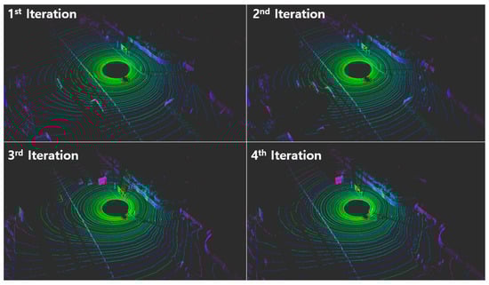
Figure 12. LiDAR scan for each iteration with different surroundings.

Comparing the RMSE in the first fifth of the course, where there were fewer parked cars and more moving cars, the RMSE of NDT matching with moveable objects was 0.1970, and the RMSE of NDT matching without moveable objects was 0.1752. The improvement rate of the mapping and matching performance of our proposed NDT was approximately 12%. The improvement rate is expected to increase in circumstances where there are more moving vehicles and fewer parked vehicles.

6. Conclusions

We cannot perform GPS-based localization accurately in certain areas, such as underground, in tunnels, and in cities with tall buildings. Therefore, we propose LiDAR-based NDT mapping and localization, which have reliable performance in areas where GPS errors are possible. The proposed method of NDT localization by removing moveable objects had 12% better performance for a specific test area with more moving vehicles.

In the future, we plan to implement the updated NDT algorithm, removing only moving objects and not deleting whole moveable objects, especially parked cars, which are a good feature for NDT mapping. We expect that the new updated algorithm, combining the JPDA-IMM-UKF algorithm, could bring out the best performance.

References

- Xia, X.; Meng, Z.; Han, X.; Li, H.; Tsukiji, T.; Xu, R.; Ma, J. An automated driving systems data acquisition and analytics platform. Transp. Res. Part C Emerg. Technol. 2023, 151, 104120. [Google Scholar] [CrossRef]
- Xia, X.; Bhatt, N.; Khajepour, A.; Hashemi, E. Integrated inertial-LiDAR-based map matching localization for varying environments. IEEE Trans. Intell. Veh. 2023. [Google Scholar] [CrossRef]
- Jo, K.; Chu, K.; Sunwoo, M. GPS-Bias Correction for Precise Localization of Autonomous Vehicles. In Proceedings of the 2013 IEEE Intelligent Vehicles Symposium (IV), Gold Coast, Australia, 23–26 June 2013; pp. 636–641. [Google Scholar]
- Peter, B.; Wolfgang, S. The Normal Distributions Transform: A New Approach to Laser Scan Matching. In Proceedings of the 2003 IEEE/RSJ International Conference on Intelligent Robots and Systems (IROS 2003) (Cat. No.03CH37453), Las Vegas, NV, USA, 27–31 October 2003; Volume 3, pp. 2743–2748. [Google Scholar]
- Takubo, T.; Kaminade, T.; Mae, Y.; Ohara, K.; Arai, T. NDT scan matching method for high resolution grid map. In Proceedings of the 2009 IEEE/RSJ International Conference on Intelligent Robots and Systems, St. Louis, MO, USA, 10–15 October 2009; pp. 1517–1522. [Google Scholar]
- Chen, S.; Ma, H.; Jiang, C. NDT-LOAM: A Real-Time LiDAR Odometry and Mapping with Weighted NDT and LFA. IEEE Sens. J. 2022, 22, 3660–3671. [Google Scholar] [CrossRef]
- Kang, D.; Wong, A.; Lee, B.; Kim, J. Real-Time Semantic Segmentation of 3D Point Cloud for Autonomous Driving. Electronics 2021, 10, 1960. [Google Scholar] [CrossRef]
- Kirillov, A.; He, K.; Girshick, R.; Rother, C.; Dollár, P. Panoptic segmentation. In Proceedings of the IEEE/CVF Conference on Computer Vision and Pattern Recognition, Long Beach, CA, USA, 15–20 June 2019; pp. 9404–9413. [Google Scholar]
- Baek, S.; Kim, M.; Suddamalla, U.; Wong, A.; Lee, B.; Kim, J. Real-Time Lane Detection Based on Deep Learning. J. Electr. Eng. Technol. 2022, 17, 655–664. [Google Scholar] [CrossRef]
- Redmon, J.; Divvala, S.; Girshick, R.; Farhadi, A. You only look once: Unified, real-time object detection. In Proceedings of the IEEE Conference on Computer Vision and Pattern Recognition, Las Vegas, NV, USA, 27–30 June 2016; pp. 779–788. [Google Scholar]
- Girshick, R. Fast r-cnn. In Proceedings of the IEEE International Conference on Computer Vision, Santiago, Chile, 11–18 December 2015; pp. 1440–1448. [Google Scholar]
- Chen, L.; Papandreou, G.; Kokkinos, I.; Murphy, K.; Yuille, A. Deeplab: Semantic image segmentation with deep convolutional nets, atrous convolution, and fully connected crfs. IEEE Trans. Pattern Anal. Mach. Intell. 2017, 40, 834–848. [Google Scholar] [CrossRef] [PubMed]
- Xiong, Y.; Liao, R.; Zhao, H.; Hu, R.; Bai, M.; Yumer, E.; Urtasun, R. Upsnet: A Unified Panoptic Segmentation Network. In Proceedings of the IEEE/CVF Conference on Computer Vision and Pattern Recognition, Long Beach, CA, USA, 15–20 June 2019; pp. 8818–8826. [Google Scholar]
- Kang, D. Object Detection by Matching Data Representation of LiDAR and Camera. Ph.D. Thesis, Graduate School of Automotive Engineering, Kookmin University, Seoul, Republic of Korea, 2023. [Google Scholar]
- Milioto, A.; Vizzo, I.; Behley, J.; Stachniss, C. RangeNet++: Fast and Accurate LiDAR Semantic Segmentation. In Proceedings of the IEEE/RSJ International Conference on Intelligent Robots and Systems (IROS), Macau, China, 3–8 November 2019; pp. 4213–4220. [Google Scholar]
- Pendleton, S.D.; Andersen, H.; Du, X.; Shen, X.; Meghjani, M.; Eng, Y.H.; Rus, D.; Ang, M.H. Perception, Planning, Control, and Coordination for Autonomous Vehicles. Machines 2017, 5, 6. [Google Scholar] [CrossRef]
- Laconte, J.; Kasmi, A.; Aufrère, R.; Vaidis, M.; Chapuis, R. A Survey of Localization Methods for Autonomous Vehicles in Highway Scenarios. Sensors 2022, 22, 247. [Google Scholar] [CrossRef] [PubMed]
- Yihuan, Z.; Liang, W.; Jun, W. Real-time localization method for autonomous vehicle using 3DLIDAR. Dyn. Veh. Roads Tracks 2017, 1, 271–276. [Google Scholar]
- Jens, B.; Cyrill, S. Efficient Surfel-Based SLAM using 3D Laser Range Data in Urban Environments. In Proceeding of Robotics: Science and System XIV, Pittsburgh, PA, USA, 26–30 June 2018; pp. 59–69. [Google Scholar]
- Andres, M.; Ignacio, V.; Jens, B.; Cyrill, S. SuMa++: Efficient LiDAR-based Semantic SLAM. In Proceedings of the IEEE/RSJ International Conference on Intelligent Robots and Systems (IROS), Macau, China, 3–8 November 2019; pp. 4530–4537. [Google Scholar]
- Kenji, K.; Jun, M.; Emanuele, M. A Portable 3D LiDAR-based System for Long-term and Wide-area People Behavior Measurement. Int. J. Adv. Robot. Syst. 2019, 16, 1729881419841532. [Google Scholar]
- Kim, M.; Kwon, O.; Kim, J. Vehicle to Infrastructure-Based LiDAR Localization Method for Autonomous Vehicles. Electronics 2023, 12, 2684. [Google Scholar] [CrossRef]
- Pagad, S.; Agarwal, D.; Narayanan, S.; Rangan, K.; Kim, H.; Yalla, G. Robust method for removing dynamic objects from point clouds. In Proceedings of the 2020 IEEE International Conference on Robotics and Automation (ICRA), Paris, France, 31 May–31 August 2020; pp. 10765–10771. [Google Scholar]
- Suleymanov, T.; Gadd, M.; Kunze, L.; Newman, P. LiDAR lateral localisation despite challenging occlusion from traffic. In Proceedings of the 2020 IEEE/ION Position, Location and Navigation Symposium (PLANS), Portland, OR, USA, 20–23 April 2020; pp. 334–341. [Google Scholar]
- Ding, P.; Wang, Z. 3D LiDAR point cloud loop detection based on dynamic object removal. In Proceedings of the 2021 IEEE International Conference on Real-time Computing and Robotics (RCAR), Xining, China, 15–19 July 2021; pp. 980–985. [Google Scholar]
- Arora, M.; Wiesmann, L.; Chen, X.; Stachniss, C. Mapping the static parts of dynamic scenes from 3D LiDAR point clouds exploiting ground segmentation. In Proceedings of the 2021 European Conference on Mobile Robots (ECMR), Bonn, Germany, 31 August–3 September 2021; pp. 1–6. [Google Scholar]
- Wissem, S.; Yacine, M.; Mohand, S.D. Multiple Sensors and JPDA-IMM-UKF Algorithm for Tracking Multiple Maneuvering Targets. Int. J. Electr. Comput. Eng. 2007, 1, 1494–1499. [Google Scholar]
- Niku, S.N. Introduction to Robotics Analysis, Systems, Applications; Pearson Education: San Luis Obispo, CA, USA, 2001; pp. 55–61. [Google Scholar]
Disclaimer/Publisher’s Note: The statements, opinions and data contained in all publications are solely those of the individual author(s) and contributor(s) and not of MDPI and/or the editor(s). MDPI and/or the editor(s) disclaim responsibility for any injury to people or property resulting from any ideas, methods, instructions or products referred to in the content. |
© 2023 by the authors. Licensee MDPI, Basel, Switzerland. This article is an open access article distributed under the terms and conditions of the Creative Commons Attribution (CC BY) license (https://creativecommons.org/licenses/by/4.0/).