

Prex-Net: Progressive Exploration Network Using Efficient Channel Fusion for Light Field Reconstruction


Abstract
:1. Introduction
- The proposed Prex-Net not only does not perform warping using depth images but also does not require pre-processing for initial feature extraction or post-processing for LF image improvement; thus, it quickly reconstructs LF images;
- For high-quality LF reconstruction, we use 3D convolution for initial feature extraction and progressively explore successive fusion groups to efficiently retrieve meaningful information existing between channels.
2. Related Works
2.1. Depth-Dependent LF Reconstruction
2.2. Depth-Independent LF Reconstruction
3. Proposed Network
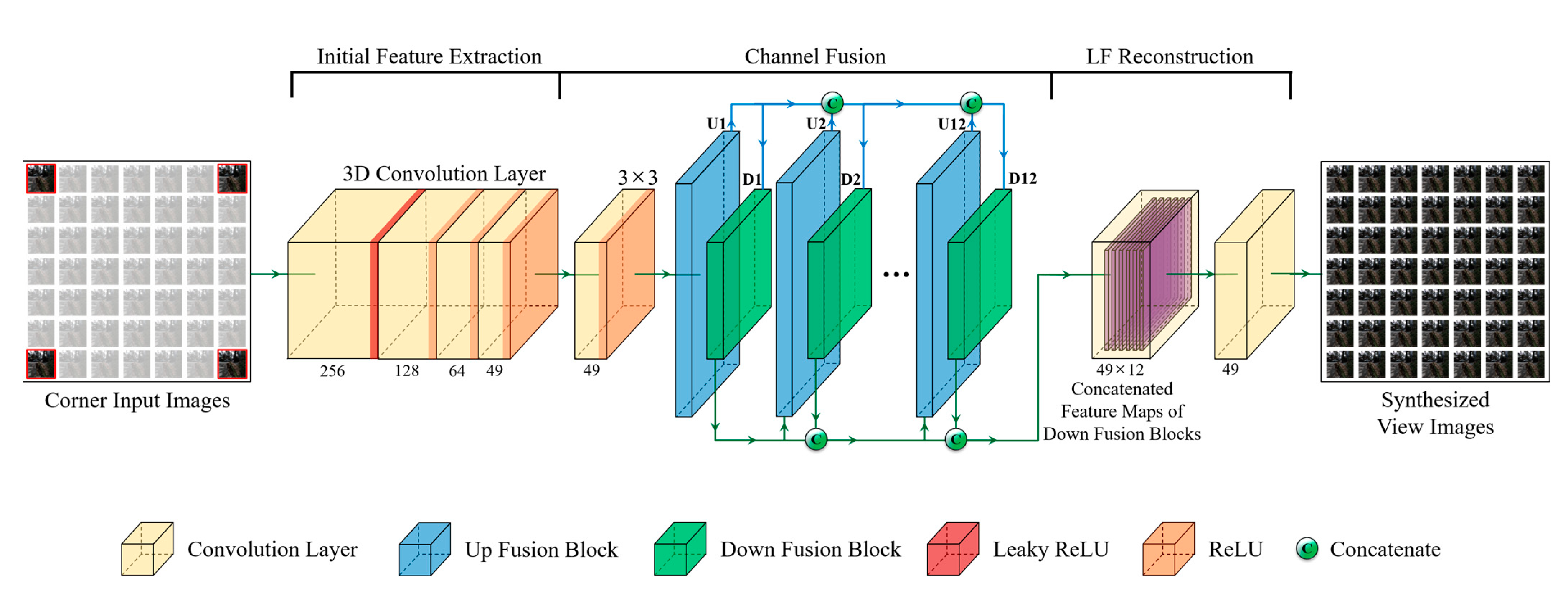
3.1. Overview
3.2. Initial Feature Extraction
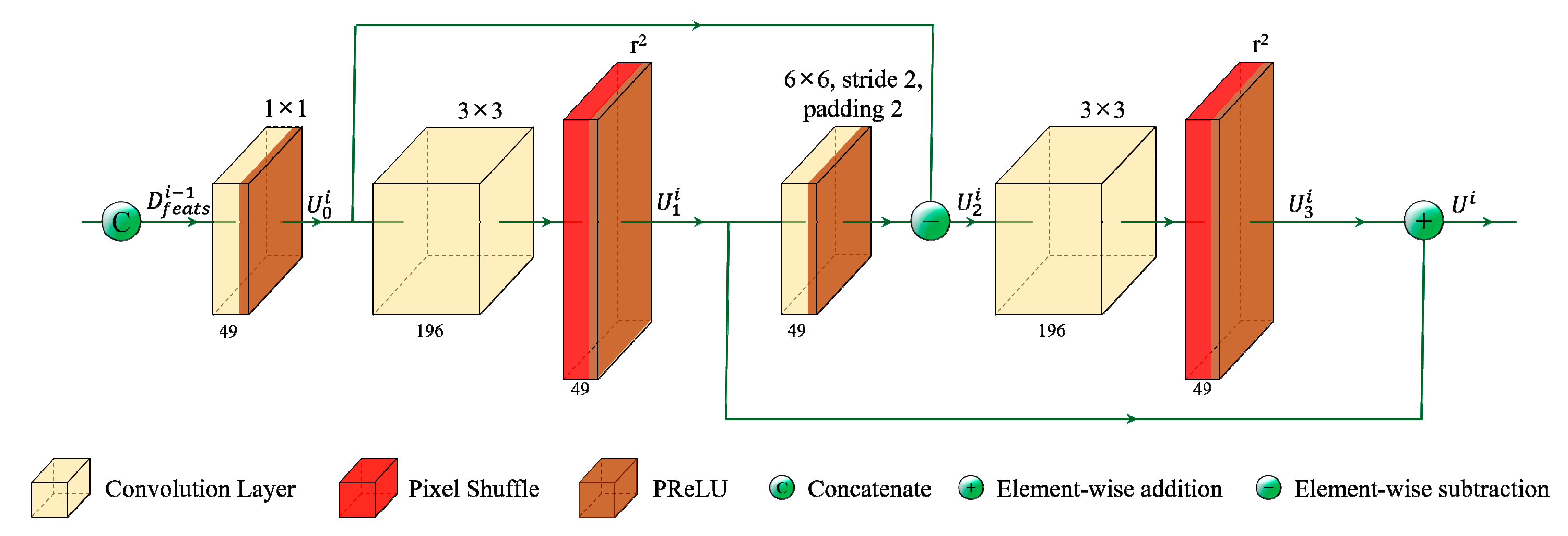
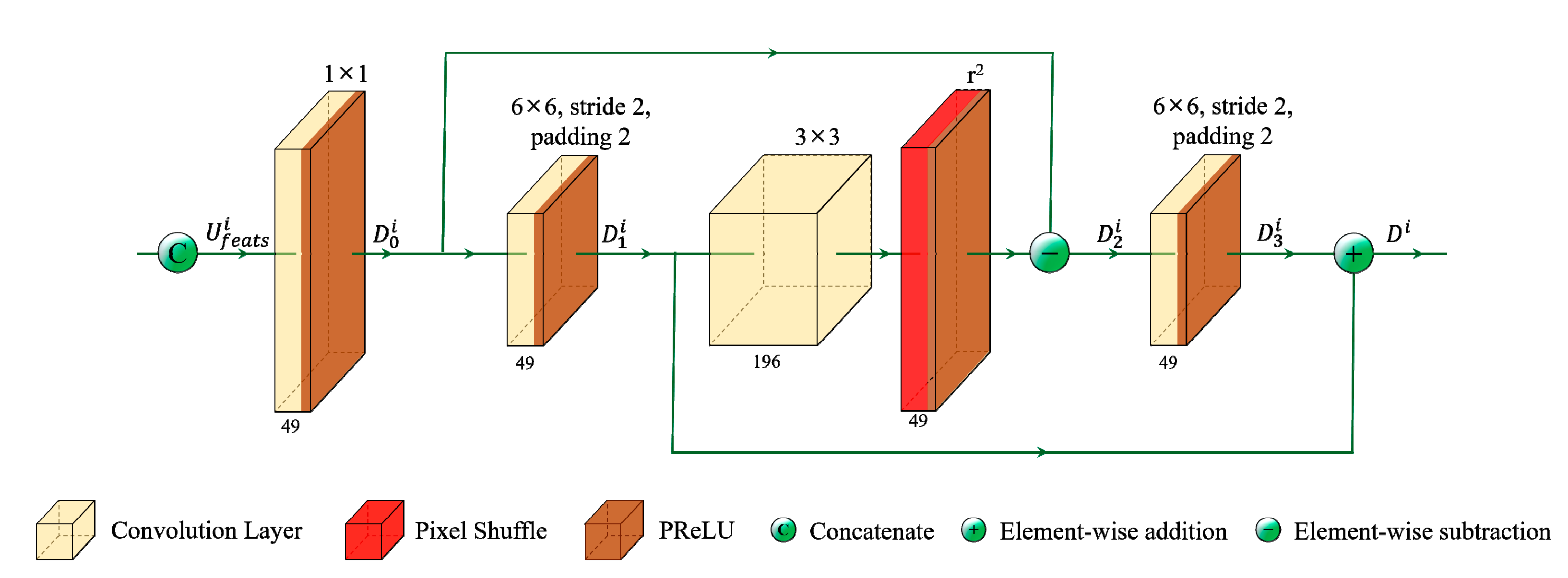
3.3. Channel Fusion Module
3.4. LF Reconstruction
4. Experimental Results
4.1. Datasets and Implementation Details
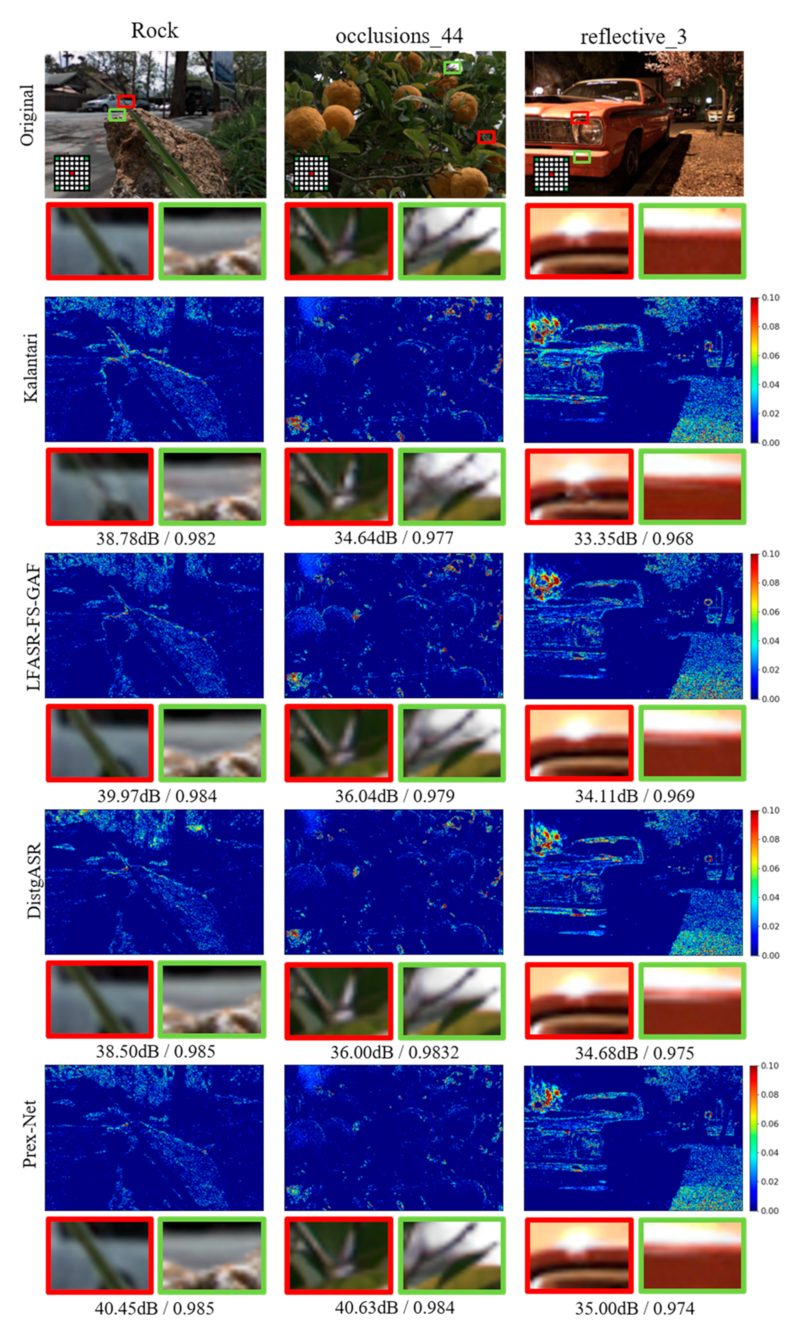
4.2. Comparison with State-of-the-Art Methods
4.3. Runtime Evaluation
4.4. Ablation Study
4.4.1. Number of Fusion Groups
4.4.2. Filter Size
5. Conclusions
Author Contributions
Funding
Institutional Review Board Statement
Informed Consent Statement
Data Availability Statement
Acknowledgments
Conflicts of Interest
References
- Wang, Y.; Yang, J.; Guo, Y.; Xiao, C.; An, W. Selective light field refocusing for camera arrays using bokeh rendering and superresolution. IEEE Signal Process. Lett. 2018, 26, 204–208. [Google Scholar] [CrossRef]
- Zhang, C.; Hou, G.; Zhang, Z.; Sun, Z.; Tan, T. Efficient auto-refocusing for light field camera. Pattern Recognit. 2018, 81, 176–189. [Google Scholar] [CrossRef]
- Kim, C.; Zimmer, H.; Pritch, Y.; Sorkine-Hornung, A.; Gross, M.H. Scene reconstruction from high spatio-angular resolution light fields. ACM Trans. Graph. 2013, 32, 73:1–73:12. [Google Scholar] [CrossRef]
- Jeon, H.G.; Park, J.; Choe, G.; Park, J.; Bok, Y.; Tai, Y.W.; So Kweon, I. Accurate depth map estimation from a lenslet light field camera. In Proceedings of the IEEE Conference on Computer Vision and Pattern Recognition, Boston, MA, USA, 7–12 June 2015; pp. 1547–1555. [Google Scholar] [CrossRef]
- Wang, T.C.; Efros, A.A.; Ramamoorthi, R. Occlusion-aware depth estimation using light-field cameras. In Proceedings of the IEEE International Conference on Computer Vision, Santiago, Chile, 7–13 December 2015; pp. 3487–3495. [Google Scholar] [CrossRef]
- Wanner, S.; Goldluecke, B. Variational light field analysis for disparity estimation and super-resolution. IEEE Trans. Pattern Anal. Mach. Intell. 2013, 36, 606–619. [Google Scholar] [CrossRef] [PubMed]
- Mitra, K.; Veeraraghavan, A. Light field denoising, light field superresolution and stereo camera based refocussing using a GMM light field patch prior. In Proceedings of the 2012 IEEE Computer Society Conference on Computer Vision and Pattern Recognition Workshops, Providence, RI, USA, 16–21 June 2012; pp. 22–28. [Google Scholar] [CrossRef]
- Le Pendu, M.; Guillemot, C.; Smolic, A. A fourier disparity layer representation for light fields. IEEE Trans. Image Process. 2019, 28, 5740–5753. [Google Scholar] [CrossRef] [PubMed]
- Flynn, J.; Neulander, I.; Philbin, J.; Snavely, N. Deepstereo: Learning to predict new views from the world’s imagery. In Proceedings of the IEEE Conference on Computer Vision and Pattern Recognition, Las Vegas, NV, USA, 27–30 June 2016; pp. 5515–5524. [Google Scholar] [CrossRef]
- Kalantari, N.K.; Wang, T.C.; Ramamoorthi, R. Learning-based view synthesis for light field cameras. ACM Trans. Graph. 2016, 35, 1–10. [Google Scholar] [CrossRef]
- Jin, J.; Hou, J.; Yuan, H.; Kwong, S. Learning light field angular super-resolution via a geometry-aware network. In Proceedings of the AAAI Conference on Artificial Intelligence, New York, NY, USA, 7–12 February 2020; pp. 11141–11148. [Google Scholar] [CrossRef]
- Jin, J.; Hou, J.; Chen, J.; Zeng, H.; Kwong, S.; Yu, J. Deep coarse-to-fine dense light field reconstruction with flexible sampling and geometry-aware fusion. IEEE Trans. Pattern Anal. Mach. Intell. 2020, 44, 1819–1836. [Google Scholar] [CrossRef] [PubMed]
- Shi, L.; Hassanieh, H.; Davis, A.; Katabi, D.; Durand, F. Light field reconstruction using sparsity in the continuous fourier domain. ACM Trans. Graph. 2014, 34, 1–13. [Google Scholar] [CrossRef]
- Vagharshakyan, S.; Bregovic, R.; Gotchev, A. Light field reconstruction using shearlet transform. IEEE Trans. Pattern Anal. Mach. Intell. 2017, 40, 133–147. [Google Scholar] [CrossRef] [PubMed]
- Yoon, Y.; Jeon, H.G.; Yoo, D.; Lee, J.Y.; Kweon, I.S. Light-field image super-resolution using convolutional neural network. IEEE Signal Process. Lett. 2017, 24, 848–852. [Google Scholar] [CrossRef]
- Gul, M.S.K.; Gunturk, B.K. Spatial and angular resolution enhancement of light fields using convolutional neural networks. IEEE Trans. Image Process. 2018, 27, 2146–2159. [Google Scholar] [CrossRef] [PubMed]
- Wang, Y.; Liu, F.; Wang, Z.; Hou, G.; Sun, Z.; Tan, T. End-to-end view synthesis for light field imaging with pseudo 4DCNN. In Proceedings of the European Conference on Computer Vision (ECCV), Munich, Germany, 8–14 September 2018; pp. 333–348. [Google Scholar] [CrossRef]
- Yeung, H.W.F.; Hou, J.; Chen, J.; Chung, Y.Y.; Chen, X. Fast light field reconstruction with deep coarse-to-fine modeling of spatial-angular clues. In Proceedings of the European Conference on Computer Vision (ECCV), Munich, Germany, 8–14 September 2018; pp. 137–152. [Google Scholar] [CrossRef]
- Wu, G.; Zhao, M.; Wang, L.; Dai, Q.; Chai, T.; Liu, Y. Light field reconstruction using deep convolutional network on EPI. In Proceedings of the IEEE Conference on Computer Vision and Pattern Recognition, Honolulu, HI, USA, 21–26 July 2017; pp. 6319–6327. [Google Scholar] [CrossRef]
- Wu, G.; Liu, Y.; Dai, Q.; Chai, T. Learning sheared EPI structure for light field reconstruction. IEEE Trans. Image Process. 2019, 28, 3261–3273. [Google Scholar] [CrossRef] [PubMed]
- Wang, Y.; Wang, L.; Wu, G.; Yang, J.; An, W.; Yu, J.; Guo, Y. Disentangling light fields for super-resolution and disparity estimation. IEEE Trans. Pattern Anal. Mach. Intell. 2022, 45, 425–444. [Google Scholar] [CrossRef] [PubMed]
- Kim, D.M.; Kang, H.S.; Hong, J.E.; Suh, J.W. Light field angular super-resolution using convolutional neural network with residual network. In Proceedings of the 2019 Eleventh International Conference on Ubiquitous and Future Networks (ICUFN), Zagreb, Croatia, 2–5 July 2019; pp. 595–597. [Google Scholar] [CrossRef]
- Haris, M.; Shakhnarovich, G.; Ukita, N. Deep back-projection networks for super-resolution. In Proceedings of the IEEE Conference on Computer Vision and Pattern Recognition, Salt Lake City, UT, USA, 18–23 June 2018; pp. 1664–1673. [Google Scholar] [CrossRef]
- Tran, D.; Bourdev, L.; Fergus, R.; Torresani, L.; Paluri, M. Learning spatiotemporal features with 3d convolutional networks. In Proceedings of the IEEE International Conference on Computer Vision, Santiago, Chile, 7–13 December 2015; pp. 4489–4497. [Google Scholar] [CrossRef]
- Sakkos, D.; Liu, H.; Han, J.; Shao, L. End-to-end video background subtraction with 3d convolutional neural networks. Multimed. Tools Appl. 2018, 77, 23023–23041. [Google Scholar] [CrossRef]
- Maqsood, R.; Bajwa, U.I.; Saleem, G.; Raza, R.H.; Anwar, M.W. Anomaly recognition from surveillance videos using 3D convolution neural network. Multimed. Tools Appl. 2021, 80, 18693–18716. [Google Scholar] [CrossRef]
- Xu, B.; Wang, N.; Chen, T.; Li, M. Empirical evaluation of rectified activations in convolutional network. arXiv 2015, arXiv:1505.00853. [Google Scholar]
- Szegedy, C.; Liu, W.; Jia, Y.; Sermanet, P.; Reed, S.; Anguelov, D.; Erhan, D.; Vanhoucke, V.; Rabinovich, A. Going deeper with convolutions. In Proceedings of the IEEE Conference on Computer Vision and Pattern Recognition, Boston, MA, USA, 7–12 June 2015; pp. 1–9. [Google Scholar] [CrossRef]
- Shi, W.; Caballero, J.; Huszár, F.; Totz, J.; Aitken, A.P.; Bishop, R.; Rueckert, D.; Wang, Z. Real-time single image and video super-resolution using an efficient sub-pixel convolutional neural network. In Proceedings of the IEEE Conference on Computer Vision and Pattern Recognition, Las Vegas, NV, USA, 27–30 June 2016; pp. 1874–1883. [Google Scholar] [CrossRef]
- Wang, L.; Wang, Y.; Lin, Z.; Yang, J.; An, W.; Guo, Y. Learning a single network for scale-arbitrary super-resolution. In Proceedings of the IEEE/CVF International Conference on Computer Vision, Montreal, QC, Canada, 10–17 October 2021; pp. 4801–4810. [Google Scholar] [CrossRef]
- Zhao, H.; Kong, X.; He, J.; Qiao, Y.; Dong, C. Efficient image super-resolution using pixel attention. In Proceedings of the Computer Vision–ECCV 2020 Workshops, Glasgow, UK, 23–28 August 2020; pp. 56–72. [Google Scholar] [CrossRef]
- Charbonnier, P.; Blanc-Feraud, L.; Aubert, G.; Barlaud, M. Two deterministic half-quadratic regularization algorithms for computed imaging. In Proceedings of the 1st International Conference on Image Processing, Austin, TX, USA, 13–16 November 1994; pp. 168–172. [Google Scholar] [CrossRef]
- Lai, W.S.; Huang, J.B.; Ahuja, N.; Yang, M.H. Deep laplacian pyramid networks for fast and accurate super-resolution. In Proceedings of the IEEE Conference on Computer Vision and Pattern Recognition, Honolulu, HI, USA, 21–26 July 2017; pp. 624–632. [Google Scholar] [CrossRef]
- Raj, A.S.; Lowney, M.; Shah, R.; Wetzstein, G. Stanford Lytro Light Field Archive; Stanford Computational Imaging Lab: Stanford, CA, USA, 2016. [Google Scholar]
- Kingma, D.P.; Ba, J. Adam: A method for stochastic optimization. arXiv 2014, arXiv:1412.6980. [Google Scholar]
- He, K.; Zhang, X.; Ren, S.; Sun, J. Deep residual learning for image recognition. In Proceedings of the IEEE Conference on Computer Vision and Pattern Recognition, Las Vegas, NV, USA, 27–30 June 2016; pp. 770–778. [Google Scholar] [CrossRef]
- Huang, G.; Liu, Z.; Van Der Maaten, L.; Weinberger, K.Q. Densely connected convolutional networks. In Proceedings of the IEEE Conference on Computer Vision and Pattern Recognition, Honolulu, HI, USA, 21–26 July 2017; pp. 4700–4708. [Google Scholar] [CrossRef]

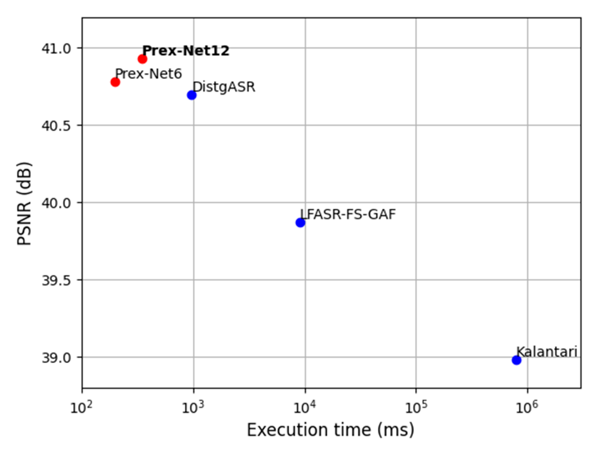
| Method | 30Scenes | Occlusions | Reflective | Average |
|---|---|---|---|---|
| Kalantari et al. [10] | 41.42/0.984 | 37.46/0.974 | 38.07/0.953 | 38.98/0.970 |
| LFASR-FS-GAF [12] | 42.75/0.986 | 38.51/0.979 | 38.35/0.957 | 39.87/0.974 |
| DistgASR [21] | 43.61/0.995 | 39.44/0.991 | 39.05/0.977 | 40.70/0.988 |
| Prex-Net (Group 6) | 43.39/0.987 | 39.70/0.982 | 39.26/0.960 | 40.78/0.976 |
| Prex-Net (Group 12) | 43.49/0.987 | 40.00/0.983 | 39.30/0.961 | 40.93/0.977 |
| Number of Groups | 30Scenes | Occlusions | Reflective | Average |
|---|---|---|---|---|
| Group 3 | 43.13 | 39.37 | 38.83 | 40.44 |
| Group 6 | 43.39 | 39.70 | 39.26 | 40.78 |
| Group 9 | 43.42 | 39.86 | 39.25 | 40.84 |
| Group 12 | 43.49 | 40.00 | 39.30 | 40.93 |
| Group 15 | 43.49 | 40.03 | 39.41 | 40.98 |
| Number of Groups | Execution Time (ms) | Parameters (M) |
|---|---|---|
| Group 3 | 140 | 2.89 |
| Group 6 | 198 | 4.58 |
| Group 9 | 254 | 6.31 |
| Group 12 | 347 | 8.08 |
| Group 15 | 435 | 9.90 |
| Filter Size | 30Scenes | Occlusions | Reflective | Average |
|---|---|---|---|---|
| 4 × 4 | 43.55 | 39.96 | 39.15 | 40.89 |
| 6 × 6 | 43.49 | 40.00 | 39.30 | 40.93 |
| 8 × 8 | 43.48 | 40.04 | 39.43 | 40.98 |
Disclaimer/Publisher’s Note: The statements, opinions and data contained in all publications are solely those of the individual author(s) and contributor(s) and not of MDPI and/or the editor(s). MDPI and/or the editor(s) disclaim responsibility for any injury to people or property resulting from any ideas, methods, instructions or products referred to in the content. |
© 2023 by the authors. Licensee MDPI, Basel, Switzerland. This article is an open access article distributed under the terms and conditions of the Creative Commons Attribution (CC BY) license (https://creativecommons.org/licenses/by/4.0/).
Share and Cite
Kim, D.-M.; Yoon, Y.-S.; Ban, Y.; Suh, J.-W. Prex-Net: Progressive Exploration Network Using Efficient Channel Fusion for Light Field Reconstruction. Electronics 2023, 12, 4661. https://doi.org/10.3390/electronics12224661
Kim D-M, Yoon Y-S, Ban Y, Suh J-W. Prex-Net: Progressive Exploration Network Using Efficient Channel Fusion for Light Field Reconstruction. Electronics. 2023; 12(22):4661. https://doi.org/10.3390/electronics12224661
Chicago/Turabian StyleKim, Dong-Myung, Young-Suk Yoon, Yuseok Ban, and Jae-Won Suh. 2023. "Prex-Net: Progressive Exploration Network Using Efficient Channel Fusion for Light Field Reconstruction" Electronics 12, no. 22: 4661. https://doi.org/10.3390/electronics12224661
APA StyleKim, D.-M., Yoon, Y.-S., Ban, Y., & Suh, J.-W. (2023). Prex-Net: Progressive Exploration Network Using Efficient Channel Fusion for Light Field Reconstruction. Electronics, 12(22), 4661. https://doi.org/10.3390/electronics12224661