Classification Algorithm of 3D Pattern Film Using the Optimal Widths of a Histogram

Abstract

A recent development in marketing tools aimed at boosting sales involves the use of three-dimensional pattern films. These films are designed to captivate customers’ interest by applying 3D patterns to the surface of products. However, ensuring the quality of these produced 3D films can be quite challenging due to factors such as low contrast and unclear layout. Furthermore, there has been a shortage of research on methods for evaluating the quality of 3D pattern films, and existing approaches have often failed to yield satisfactory results. To address this pressing issue, we propose an algorithm for classifying 3D pattern films into either ‘good’ or ‘bad’ categories. Unlike conventional segmentation algorithm or edge detection methods, our proposed algorithm leverages the width information at specific heights of the image histograms. The experimental results demonstrate a significant disparity in histogram shapes between good and bad patterns. Specifically, by comparing the widths of all images at the quintile of the histogram height, we show that it is possible to achieve a 100% accuracy in classifying patterns as either ‘good’ or ‘bad’. In comparative experiments, our proposed algorithm consistently outperformed other methods, achieving the highest classification accuracy.

1. Introduction

A manufacturing company has recently developed 3D pattern films that show a three-dimensional appearance. These intricate patterns are intended for application on various product surfaces such as cosmetics, perfumes, wallpapers, and more, serving as a powerful marketing tool to capture the attention of potential buyers, as illustrated in Figure 1. The 3D pattern film is a product achieved by adjusting the concentration of 2D film ink, as shown in Figure 2. When printed, these 3D pattern films show slight variations in appearance based on factors like viewing angles, brightness, light intensity, and the observer’s perspective, as demonstrated in Figure 3.

Figure 1. Production goods with 3D film images attached.

Figure 2. Two types of 3D pattern film. (a) Good pattern; (b) Bad pattern.

Figure 3. Three-dimensional pattern film image production. (a) Production machine; (b) manufacturing process.

As shown in Figure 3, the 3D pattern film images are produced using a manufacturing machine, subsequently transferred to an inspection apparatus, and captured by a camera. Following this, the captured 3D pattern film images undergo a thorough quality inspection, with patterns being categorized as either ‘good’ or ‘bad’ based on pattern evaluations. If a 3D pattern film is classified as good, it is then applied to product surfaces, as exemplified in Figure 1. However, a significant need exists for a quality inspection algorithm within the quality control system to identify defects in 3D films for sales purposes, since one has not been developed yet.

Figure 2a shows a good 3D pattern film, while Figure 2b displays a bad 3D pattern film. Although the manufacturer plans to produce various patterns, the initial 3D film to be produced is shown in Figure 2. This pattern is characterized by varying sizes and textures. The good 3D pattern film image in Figure 2a shows clear contours and high-contrast pixels. In contrast, the bad 3D pattern film image in Figure 2b displays blurred contours and low-contrast pixels in the pattern. Consequently, when a bad 3D pattern film is applied to a product surface, the printed pattern appears blurry, lacking the three-dimensional effect and making pattern recognition challenging. Therefore, it becomes imperative to assess pattern quality once it is printed on the 3D pattern film.

To analyze 3D pattern films, a range of inspection methods such as shape, texture, similarity, and contrast, as found in existing algorithms, can be employed [1,2,3,4,5,6,7,8,9,10,11,12,13,14,15,16,17,18]. Segmentation algorithms may be considered for analyzing the shape of 3D pattern films, while edge detection algorithms can be applied to study texture. Additionally, algorithms based on the absolute difference can be used to determine the similarity between good 3D pattern film samples and new products, along with considering the brightness and luminosity attributes of 3D pattern films. However, even with these algorithms, obtaining satisfactory results remains challenging, largely due to the scarcity of research concerning 3D pattern film images.

In this paper, we propose an algorithm for defect detection of 3D pattern film images from a statistical perspective. The algorithm classifies good and bad 3D pattern film images using the width at the specific height of the histogram of a 3D pattern film image. The proposed algorithm process has the advantage of not requiring pattern segmentation and instead calculates the width from the histogram of the image, making the calculation process less complex. The remainder of this paper is organized as follows: Section 2 describes conventional and recently published methods for classifying good and bad images. Section 3 describes the algorithm proposed in this paper, and Section 4 presents the experimental results obtained using the proposed algorithm. Specifically, since suitable methodologies vary for each dataset, we compared both traditional and recently published methods. Finally, Section 5 presents the conclusions of this study.

2. Related Works

Methods that can be used to detect patterns in 3D film images and classify them as good or bad 3D pattern film images include absolute-based (Abs-based) difference, binarization, segmentation, brightness contrast, luminance contrast, support vector machine (SVM), and template matching method. Abs-based difference relies on image subtraction of absolute value; it utilizes the difference between pixels of two similar or different images [1]. Binarization and edge detection methods are representative rule-based methods for segmentation that distinguishes different regions existing in an image. Binarization is a method wherein pixels with high or low value are changed to black or white based on a threshold applied to a gray image. Generally, binarization involves adaptive binarization, Otsu thresholding, etc. [2,3]. The adaptive binarization algorithm divides an image into several areas and then uses the pixel value around it to obtain a threshold. However, this algorithm is effective when the lighting changes or reflections are severe in an image, and a lot of computation is required because thresholds must be obtained for each block, and the results may vary depending on the block size and parameters. Thus, the user should determine the appropriate values for each image. Otsu thresholding involves using the histogram of the image to determine the optimal threshold and apply binarization. However, obtaining the optimal threshold value is challenging when the images to be detected are small or the difference in its distribution from the background is large. Edge detection is a method used to identify areas where the brightness of a pixel has a high rate of change and uses differentiation and derivatives of the gradient operation to detect the boundaries of an object. Therefore, the point where the brightness changes noticeably is referred to as the edge. Edge detection algorithms include Sobel edge detection, Laplacian edge detection, and Canny edge detection [4]. However, Sobel edge detection is affected by the brightness of the image, and while Laplacian edge detection detects thin lines and isolated points, it is also sensitive to noise and detects more edges than actually present. In addition, Canny edge detection is considerably affected by the threshold, making it difficult to detect the 3D film image. Recently, Mlyahilu et al. [5] published a study comparing the results of classification after performing edge detection on pattern images and classification using a convolutional neural network (CNN). In Figure 4, (a) is the pattern image used in the experiment, (b) is the edge detection result for Canny, and (c) is the edge detection result for Sobel. Figure 4b,c display the results of applying the edge detection method to image (a), and good classification results can be expected only when the pattern is well detected in this result. However, edges were not connected or naturally detected in the result shown in Figure 4b, and the detected patterns were more blurry than the original in the result shown in Figure 4c. Therefore, it can be confirmed that there is a limit to detecting a pattern using edge detection methods in a pattern image. In addition, several studies were proposed using a morphological snake that performs object detection using morphological operators such as expansion and erosion as a segmentation method [6]. The morphological geodesic active contour method in [7,8] that combines morphological snakes and geodesic active contour in [9] is used to accurately detect patterns by widening the gradually developing contour to a local minimum; this prevents the detection of other reduced minimum contours. Recently, Medeiros et al. [8] proposed a Fast Morphological Geodesic Contour (FGAC) method of segmentation without prior training using a new Fuzzy Border Detector. However, it is difficult to accurately specify the location of objects to be detected in the pattern image each time when creating bounding boxes in the morphological geodesic active content.

Figure 4. Pattern image and edge detection results from Canny and Sobel methods. (a) Image; (b) Canny; (c) Sobel.

Studies using luminance contrast methods have been proposed to distinguish patterns in the image. Among these methods, Michelson contrast in [10] uses the values obtained through the maximum luminance and minimum luminance values of the input image to compare images, and the equation is as follows:

$$M_k=\frac{X_{max}-X_{min}}{X_{max}+X_{min}},$$

(1)

where $M_k$ is the Michelson contrast value of the $k$-th input image, and $X_{min}$ and $X_{max}$ are the minimum and maximum luminance values in the input image. In addition, there is a Weber contrast in [11] that calculates the luminance ratio by dividing the difference between the maximum luminance and the minimum luminance by the minimum luminance. However, these methods cannot be guaranteed for the classification accuracy of the 3D pattern film images because they are ways to compare the difference in light and dark images if a small number of luminosity values are distributed in the good and bad pattern images as a whole.

Recently, several studies have used SVM, which classifies data based on the decision boundary. Hsu and Chen [12] proposed a method of classifying bad pattern images with blurred extent estimation and then distinguishing local and global blurs. Wang et al. [13] proposed a support vector rate (SVR) method that uses an ensemble SVM model to automatically classify good pattern images and bad pattern images whose contours are blurred with various elements. Salman et al. [14] used SVM after applying canny edge detection. However, finding a boundary to divide data in SVM is challenging, and optimal values of hyper-parameters should be identified to determine the penalty for errors. Various studies have been conducted to address the aforementioned problems, but most studies have been focused on how to identify and classify factors that blur images and how to recover bad images [15,16].

A template matching method is used to find a part in the image that matches the template image [17,18]. However, the size and direction of the template did not match those of the printed image because the printed 3D film image analyzed in this paper did not have the same size and texture. In addition, the good and bad 3D film images presented in this paper were not easy to detect because the contrast of the pixels in the images differed between them. Furthermore, solving the classification problem using existing methods is challenging because the patterns of the good and bad 3D images are similar to each other.

3. Proposed Algorithm

The 3D patterns in an image should be segmented to conduct the quality test of the 3D film image using most of the existing methods. For this purpose, it is necessary for the pattern and background to have distinct differences, and the edges of the pattern need to be clear for object detection to be possible. However, in contrast to the aforementioned good pattern images, bad pattern images have low contrast among the pixels and lack clear contours, making it challenging to detect image patterns and classify them. To solve the difficulty of existing problems, in this paper, we consider a histogram, which is a statistical method to test quality by using the fact that the contrast of each 3D film is different without segmenting the pattern. In this section, we describe how to classify 3D pattern film images into good or bad classes using the image histogram. To this end, first, each pattern is cut for the 3D film in Figure 2, and then the quality of the patterns is classified through the algorithm using image histograms.

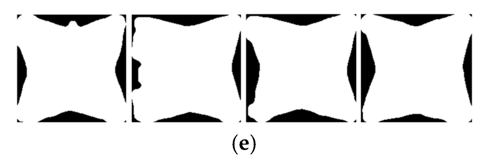
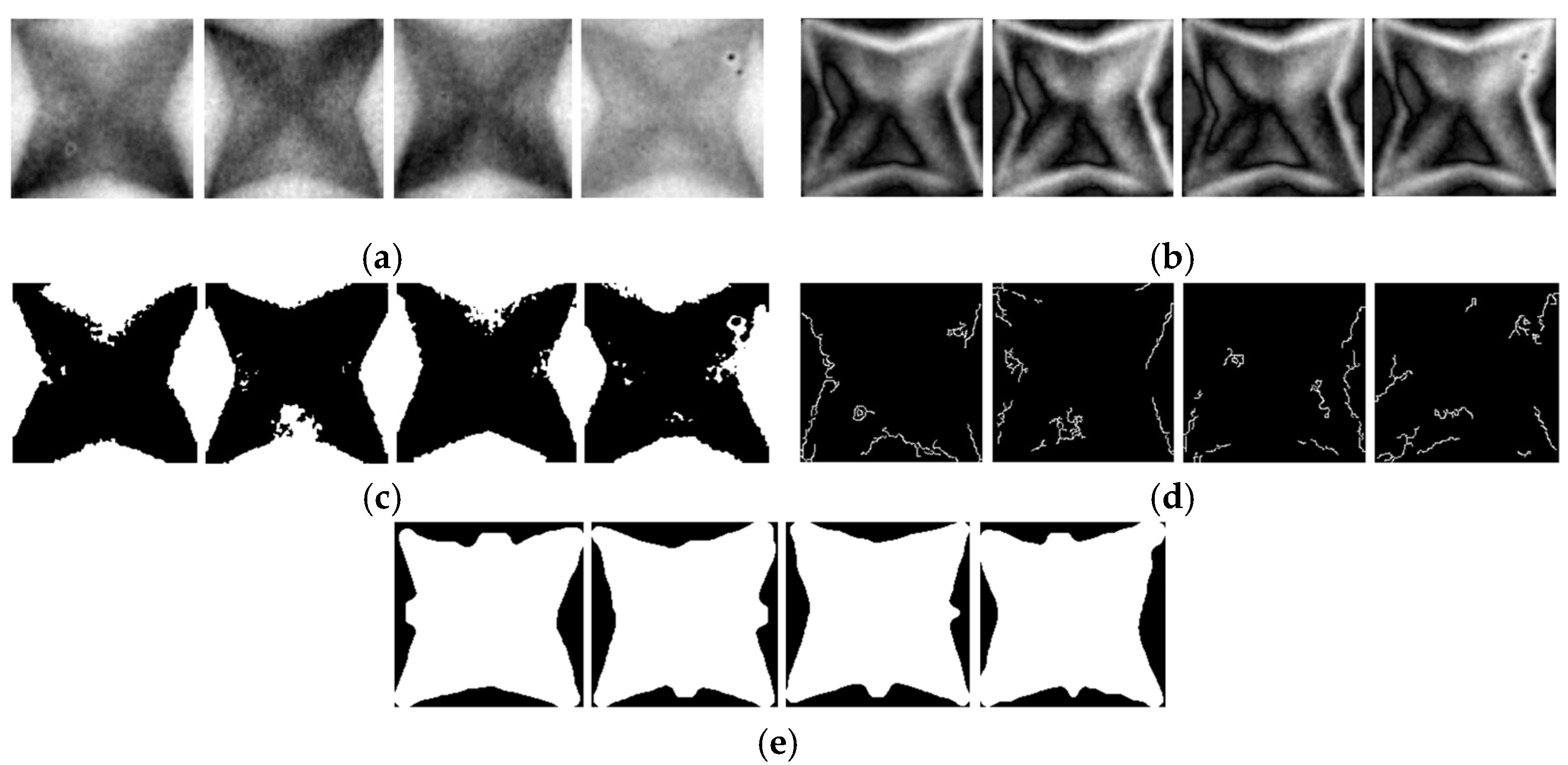
3.1. Fast Fourier Transform for Cropping 3D Pattern Film Images

To cut the pattern images individually, we use the fast Fourier transform proposed by Mlyahilu and Kim in [19] to cut the image by pattern in the printed 3D film. The 2D discrete Fourier transform (DFT) of an image $f\left(a,b\right)$ is as follows:

$$F\left(u,v\right)={{\displaystyle \sum }}_{a=0}^{N-1}{{\displaystyle \sum }}_{b=0}^{N-1}f\left(a,b\right)e^{-2\pi j\left(\frac{au}{N}+\frac{bv}{N}\right)},$$

(2)

where $f\left(a,b\right)$ of size N by N is defined for $0\le a,b\le N-1$ and the complex exponential function is expressed in terms of cosine and sine functions. The Fourier image can be transformed back into the original image through the discrete inverse Fourier transform formula as follows:

$$f\left(a,b\right)=\frac{1}{N^2}{{\displaystyle \sum }}_{u=0}^{N-1}{{\displaystyle \sum }}_{v=0}^{N-1}F\left(u,v\right)e^{2\pi j\left(\frac{au}{N}+\frac{bv}{N}\right)},$$

(3)

The equation for the 2D DFT can be decomposed into a series of 1D Fourier transforms as follows:

$$F\left(u,v\right)={{\displaystyle \sum }}_{a=0}^{N-1}F\left(a,v\right)e^{-2\pi j\left(\frac{au}{N}\right)},$$

(4)

$$F\left(a,v\right)={{\displaystyle \sum }}_{b=0}^{N-1}f\left(a,b\right)e^{-2\pi j\left(\frac{bv}{N}\right)},$$

(5)

However, 2D DFT requires a time complexity of $\mathrm{O}\left(N^4\right)$. To address this, fast Fourier transform (FFT) is performed to efficiently compute the Fourier transformation. To calculate the 2D FFT of an N $\times$ N image, the 1D FFT is first performed along the rows of the image, and then the 1D FFT is performed along the columns. Since the imaginary part is nearly zero and an image is always a real-valued function, we utilize the real part of the processed image. We determine the horizontal and vertical index of white pixel values to obtain the horizontal $I_x\left(x,y\right)$, vertical $I_y\left(x,y\right)$, as shown in Equations (6) and (7).

$$I_x\left(x,y\right)=\left\{\begin{array}{c}255, F\left(a,v\right)>0\\ 0, elsewhere\end{array}\right.,$$

(6)

$$I_y\left(x,y\right)=\left\{\begin{array}{c}255, F\left(a,v\right)>0\\ 0, elsewhere\end{array}\right.,$$

(7)

From the result of white lines in Equations (6) and (7), the pixel coordinates are obtained by the intersection. After that, the pattern images of the 3D film can be cut by using the intersection information.

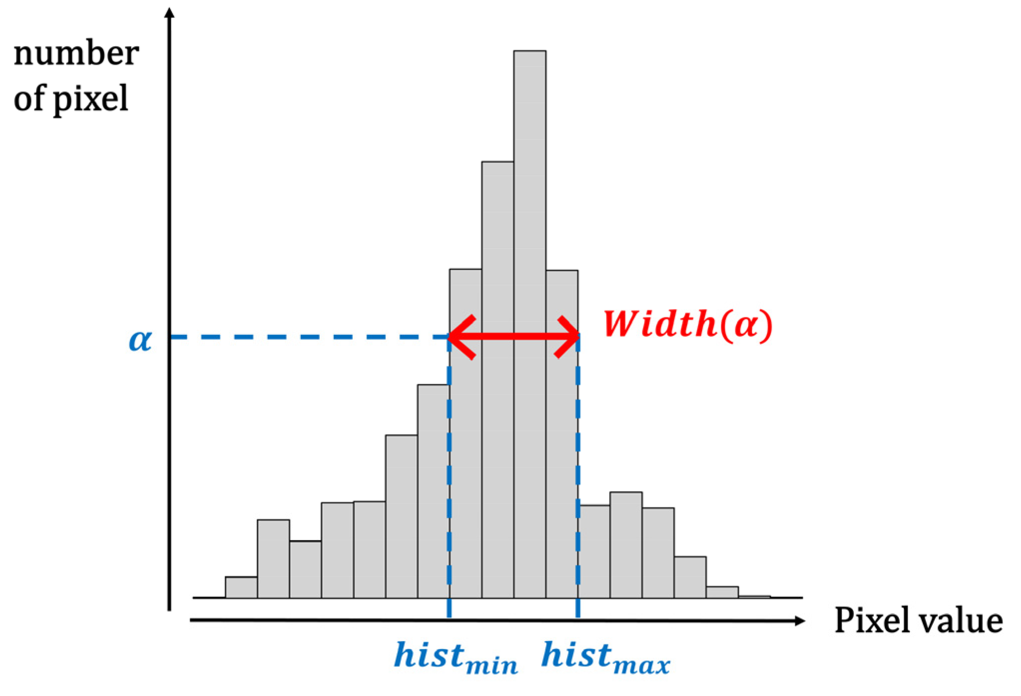
3.2. Classification for 3D Pattern Film Images Based on Widths at Specific Heights of Histogram

After applying the FFT in Section 3.1 to segment the patterns of the 3D film, the 3D pattern film images are compared and classified into good and bad pattern images based on their quality. The flow of the proposed algorithm is illustrated in Figure 5. First, we input the pattern image of the 3D film, and then calculate the histogram of the cropped image. A histogram is a visual representation of the distribution of data, and similarly, an image histogram expresses the x-axis as the pixel value and the y-axis as the frequency of the pixel. Using an image histogram, information such as that regarding the distribution of pixels in the image and the contrast of the image can be obtained; thus, histograms are widely used in image processing. The histogram for each image is displayed in Figure 6, where (a) displays the good pattern image and the histogram for the pixel value of the image, and (b) displays the bad pattern image and the histogram for the pixel value of the image. As illustrated in Figure 6, the good pattern image was wide on the x-axis, which represents the pixel value of the histogram, because the contrast of the pixel in the image was high. In comparison, the bad pattern image was narrow on the x-axis of the histogram because the contrast of the pixel in the image was low. Thus, the proposed algorithm calculates the width according to the specific height of the histogram and performs a quality test with the 3D film as good or bad. However, the reason why the width of the bottom of the histogram is not calculated is that some good pattern images have relatively narrow bottom widths, as shown in Figure 7a, while some bad pattern images have wide bottom widths, as shown in Figure 7b. Therefore, the width of the bottom of the histogram is not calculated to increase the inspection accuracy but is examined using a value of a specific height.

Figure 5. Procedures of the proposed algorithm.

Figure 6. Usual 3D pattern film images with the histogram. (a) Good pattern images; (b) bad pattern images.

Figure 7. Unusual 3D pattern film images with the histogram. (a) Good pattern images; (b) bad pattern images.

After a specific threshold α value is determined among the height of the y-axis of every histogram, the maximum value $his{t}_{\max }$ and the minimum value $his{t}_{\min }$ of the pixel value for the height $\mathsf{\alpha }$ of the histogram are obtained as shown in Equations (8) and (9).

$$his{t}_{\min }=\underset{x}{\min } f_{\alpha }\left(x\right),$$

(8)

$$his{t}_{\max }=\underset{x}{\max } f_{\alpha }\left(x\right),$$

(9)

where $f_{\alpha }\left(x\right)$ represents the pixel values $x$ at the height $\mathsf{\alpha }$ value of the image histogram in the gray image $I\left(a,b\right)$. The width of the pixel $Width\left(\alpha \right)$, which is the difference between the previously obtained $his{t}_{\max }$ and $his{t}_{\min }$, is obtained. The equation for calculating the width of the histogram is as follows:

$$Width\left(\alpha \right)=his{t}_{\max }-his{t}_{\min },$$

(10)

For this procedure, the width is calculated for all heights corresponding to the quintiles of the histogram height. The process of obtaining width ($Width\left(\alpha \right)$) is illustrated in Figure 8. Empirically, to compare all widths for the quintiles of the histogram height, values with α from 1/5 to 4/5 are obtained. In other words, if α is greater than 4/5, it implies that α has calculated the heights for all quintiles from 1/5 to 4/5. Following the aforementioned procedure, we obtain the width of all images at height $\mathsf{\alpha }$ of the histograms, calculate the minimum and maximum width ranges of each of the good and bad pattern images, and compare the overlapping images within the two ranges.

Figure 8. The $his{t}_{min}$ and $his{t}_{max}$ at specific frequency $\alpha$ in the histogram.

4. Experimental Results

To evaluate the performance of the proposed algorithm, the experiment was conducted using a total of 760 3D film images, of which 570 were good 3D film images and 190 were bad 3D film images. Figure 9 displays the data used in the experiment: (a) good 3D pattern film images and (b) bad 3D pattern film images. These images were cropped by using the fast Fourier transform for each pattern in the 3D film displayed in Figure 2, and the size of each image was 169 × 169. Figure 9 represents a collection of some of the actual products that will be sold, gathered for the purpose of developing a product quality inspection algorithm. Thus, we utilized images of these products, as shown in Figure 9, as experimental data. PC specifications were as follows: Window 10 Pro, Intel^® Core™ i7010700k CPU@3.80 GHz, NVIDIA GeForce RTX 2080 SUPER, 16 GB, and Python 3.6.

Figure 9. Cropped 3D pattern film images. (a) Good pattern images; (b) Bad pattern images.

As shown in the flow chart depicted in Figure 5, we analyzed all of the 3D film images. First, we obtained the histogram of the 3D pattern film image as shown in Figure 6. After that, the widths of the specific height of the histogram were obtained for all good and bad pattern images and the analysis results are summarized in Table 1. Table 1 displays the width at heights from one-fifth to four-fifths of the histogram for each image, and then the minimum width and the maximum width at the corresponding height were obtained for all images. The number of images overlapping with the good and bad pattern images for each height were analyzed, and the degree of classification was denoted as accuracy. As seen in Table 1, the good pattern images and defective pattern images were classified with 100% accuracy at heights of one-fifth and two-fifths of the histogram. Furthermore, at three-fifths of the height of the histogram, classification was achieved with a relatively high accuracy of 98.68%.

Table 1. Classification accuracy of 3D film images.

	Height ($\mathbf{\alpha }$)	1/5	2/5	3/5	4/5
Good pattern image	Min	125	125	28	1
	Max	227	227	196	164
Bad pattern image	Min	24	24	4	1
	Max	94	94	31	25
Number of Collapsed Images		0	0	10	348
Accuracy (%)		100	100	98.68	54.21

To evaluate the performance of the proposed algorithm, the analysis results were compared using the Abs-based difference method, Otsu thresholding, Canny edge detection, the CNN with the Canny method [5], morphological geodesic active contour [7], Michelson contrast [10], and the SVM with the Canny method [14]. For the Abs-based difference, Otsu thresholding, Canny edge detection, and morphological geodesic active control methods, a structural similarity index (SSIM) was used to evaluate the similarity between the two images [20]. SSIM helps to evaluate similarity using the structural information of two images and compares the structures of the pixels constituting the image as follows:

$$\begin{gathered} S\left(x,y\right)=l\left(x,y\right)·c\left(x,y\right)·s\left(x,y\right) \\ =4{\mu }_x{\mu }_y{\sigma }_{xy}/\left\{\left({\mu }_x^2+{\mu }_y^2\right)\left({\sigma }_x^2+{\sigma }_y^2\right)\right\}, \\ where l\left(x,y\right)=\left(2{\mu }_x{\mu }_y\right)/\left({\mu }_x^2+{\mu }_y^2\right), \\ c\left(x,y\right)=\left(2{\sigma }_x{\sigma }_y\right)/\left({\sigma }_x^2+{\sigma }_y^2\right), \\ s\left(x,y\right)=\left(2{\sigma }_{xy}\right)/\left({\sigma }_x{\sigma }_y\right) \end{gathered}$$

(11)

where $l\left(x,y\right)$, $c\left(x,y\right)$, and $s\left(x,y\right)$ represent the average brightness, contrast, and correlation of the two images, respectively. We evaluated the SSIM results using a threshold of 0.5, where a higher SSIM value indicates similarity between the two images, and a lower SSIM value indicates dissimilarity between the images. For the CNN with the Canny method proposed by Mlyahilu et al. [5], we used 32 and 64 nodes in the convolution layer, two maximum pooling layers, 10 epochs, ReLu for the activation function, and Adam for the optimization function as in the paper. In addition, the dataset was divided into a training set and a test set whereby the former had 560 images and the latter had 200 images, respectively. To evaluate the performance of the algorithms, the accuracy, recall and specificity were computed. We calculated the evaluation metrics based on the confusion matrix between the good and bad images as follows:

$$Accuracy=\left(TP+TN\right)/\left(TP+TN+FP+FN\right),$$

(12)

$$Recall=TP/\left(TP+FN\right),$$

(13)

$$Specificity=TN/\left(TN+FP\right),$$

(14)

where $TP$ is true positive, $TN$ is true negative, $FP$ is false positive, and $FN$ is false negative. Figure 10a–e display the results obtained using the proposed, Abs-based difference, Otsu thresholding, Canny edge detection, and morphological geodesic active control algorithms for the good 3D film images, respectively. In addition, Figure 11a–e display the results obtained using the same algorithms for the bad 3D film images. The Abs-based difference method determines the pixel differences between the good pattern image and the other images. In the results, the white areas represent the differences between the two images. In Canny edge detection, the minimum threshold value was set to 50, the maximum threshold value was set to 10, and the segmentation result was expressed using a segmentation mask. Among the results regarding the differences between the two good pattern images in Figure 10, it can be observed that in Figure 10b, there are slight variations in the outline and the central part of the pattern, but there is no significant difference. In addition, as shown in the results of Figure 10c,e, Otsu thresholding and morphological geodesic active contour were able to detect the contours to some extent. However, Canny edge detection detected too many edges, making it difficult to find the desired contour as shown in Figure 10d. On the other hand, Figure 11b represents the analysis results of the difference between a good pattern image and a bad pattern image. In Figure 11b, the Abs-based difference shows that there is a noticeable difference in the contours between the good images and the bad images. However, as shown in Table 2, the Abs-based difference demonstrated differences in contours, but it did not achieve high accuracy in discriminating between similar images. Figure 11c,e also managed to detect bad images to some extent. However, as observed from the results in Table 2, they did not achieve high accuracy in determining the differences between the two images. On the other hand, Figure 11d failed to detect the contour effectively. This indicates that Canny edge detection struggles to detect contours when they are blurred or unclear. Table 2 illustrates the classification results of good and bad 3D film images obtained using each conventional method and proposed algorithm. As displayed in Table 2, the computational time was the longest for morphological geodesic active contour at approximately 485.69 s, and the proposed method took approximately 54.45 s. On the other hand, other algorithms took less than 10 s for computation. The reason for the high computational time in the proposed study is due to the analysis of histograms and width calculation for each image, as well as the retrieval and comparison of stored data. However, the accuracy of the proposed algorithm was the best, at 100% when the histogram’s specific height $\mathsf{\alpha }$ was one-fifth or two-fifths, and a large difference in accuracy was observed compared with other methods. Otsu thresholding and Canny edge detection have very fast computation times, but their accuracy is within the range of 20%. In particular, Canny edge detection failed to classify any of the 3D film good pattern images. CNN with Canny had the fastest computation time at 0.954 s, but its accuracy was only 71.5%, which significantly differed from the proposed algorithm. Furthermore, Abs-based difference also showed poor performance at 54.74%, and morphological geodesic active contour and the SVM with the Canny method showed low accuracy of 70%. This is because the patterns were not properly detected in the bad pattern image, as depicted in Figure 11. Michelson contrast is a method of distinguishing patterns using luminance through a formula similar to the proposed algorithm. However, the experiment showed an accuracy of 90.53%, and 72 out of the total 760 good and bad pattern images were not classified. Therefore, through the experiments, it was observed that although the proposed algorithm had a slightly longer computation time compared to other algorithms, it exhibited a significant difference in accuracy.

Figure 10. Good pattern images obtained with algorithms. (a) Original pattern images; (b) Abs-based difference; (c) Otsu thresholding; (d) Canny edge detection; (e) morphological geodesic active contour.

Figure 11. Bad pattern images obtained with algorithms. (a) Original pattern images; (b) Abs-based difference; (c) Otsu thresholding; (d) Canny edge detection; (e) morphological geodesic active contour.

Table 2. Classification results for algorithms with 3D film images.

Algorithm	Number of Misclassified Images		Accuracy	Recall	Specificity	AUC	Time (s)
	Good Pattern	Bad Pattern
Proposed algorithm ($\mathsf{\alpha }=1/5 \mathrm{or} 2/5)$	0	0	1.0000	1.0000	1.0000	1.0000	54.450
Michelson contrast [10]	62	10	0.9053	0.8912	0.9474	0.9193	9.625
Morphological geodesic active contour [7]	101	90	0.7486	0.8228	0.5263	0.6746	485.690
Canny + SVM [14]	113	85	0.7394	0.8018	0.5526	0.6772	6.800
Canny + CNN [5]	-	-	0.7150	0.7805	0.6681	-	0.954
Abs-based difference	227	117	0.5474	0.6018	0.3842	0.4930	1.316
Otsu thresholding	368	179	0.2803	0.3544	0.5790	0.2061	1.328
Canny edge detection	570	0	0.2500	0.0000	100.00	0.5000	1.451

5. Conclusions and Discussion

The 3D film is a recently developed product and has a limitation in that there is rarely a quality inspection method that has been researched in advance. In addition, good 3D pattern film images have high contrast, whereas bad 3D pattern film images have low contrast and their external contours are not clear, making the detection of patterns during quality inspection difficult. To address this difficulty, we proposed an algorithm that classifies good and bad 3D pattern film images by comparing the pixel width at a specific height in the histogram of 3D pattern film images. The proposed algorithm classifies good or bad 3D pattern images by considering the aforementioned characteristics of 3D films. Moreover, the quality inspection algorithm can be performed experimentally by classifying pattern images at high accuracy without requiring prior information and segmentation of the image. We performed the image classification at one-fifth to four-fifths height points in the histogram of the 3D pattern film image, and the proposed algorithm showed that good and bad are classified 100% at one-fifth and two-fifths heights. In addition, we performed a comparative experiment using existing algorithms such as SVM and morphological geodesic active contour to validate the performance of the proposed algorithm. In the experimental results, the classification accuracy of existing algorithms was all less than 90%. Moreover, among the existing algorithms, Michelson contrast had the highest classification accuracy, but the accuracy was significantly different from the proposed method.

In this paper, as previously mentioned, we have presented a novel approach for quality inspection of 3D pattern film images through the proposed method, offering solutions to existing challenging issues. Additionally, through experimental results, we have demonstrated that the proposed algorithm achieves superior classification accuracy compared to existing algorithms, thus validating its utility as an effective tool for enhancing product quality. Therefore, the research findings in this paper can make a significant contribution to product quality improvement and increased productivity in the manufacturing and quality management of 3D films. Furthermore, the efficient quality inspection method presented in this paper is expected to contribute to cost savings and ensure consistent product quality.

In further research, we plan to conduct a study where, in the evaluation of product quality, we automatically find the optimal histogram height value from the method proposed in this paper and classify it into good and bad categories. In addition, we plan to reduce the computational time through the proposed algorithm optimization and study a general test method that can be used through experiments on various types of 3D pattern film images.

References

1. Mirbod, M.; Rezaei, B.; Najafi, M. Spatial change recognition model using artificial intelligence to remote sensing. Procedia Comput. Sci. 2023, 217, 62–71. [Google Scholar] [CrossRef]
2. Mustafa, W.A.; Kader, M.A. Binarization of Document Images: A Comprehensive Review. J. Phys. Conf. Ser. 2018, 1019, 012023. [Google Scholar] [CrossRef]
3. Seelaboyina, R.; Vishwakarma, R. Different Thresholding Techniques in Image Processing: A Review. In Proceedings of the ICDSMLA 2021: Proceedings 3rd International Conference on Data Science, Machine Learning and Applications, Copenhagen, Denmark, 17–18 September 2022; pp. 23–29. [Google Scholar]
4. Owotogbe, Y.S.; Ibiyemi, T.S.; Adu, B.A. Edge detection techniques on digital images—A review. Int. J. Innov. Res. Technol. 2019, 4, 329–332. [Google Scholar]
5. Mlyahilu, J.; Kim, Y.; Kim, J. Classification of 3D Film Patterns with Deep Learning. Comput. Commun. 2019, 7, 158–165. [Google Scholar] [CrossRef]
6. Álvarez, L.; Baumela, L.; Neila, P.M.; Henríquez, P. A real time morphological snakes algorithm. Image Process. Line 2014, 2, 1–7. [Google Scholar] [CrossRef]
7. Mlyahilu, J.; Mlyahilu, J.; Lee, J.; Kim, Y.; Kim, J. Morphological geodesic active contour algorithm for the segmentation of the histogram-equalized welding bead image edges. IET Image Process. 2022, 16, 2680–2696. [Google Scholar] [CrossRef]
8. Medeiros, A.G.; Guimarães, M.T.; Peixoto, S.A.; Santos, L.D.O.; da Silva Barros, A.C.; Rebouças, E.D.S.; Victor Hugo, C.D.; Rebouças Filho, P.P. A new fast morphological geodesic active contour method for lung CT image segmentation. Measure 2019, 148, 106687. [Google Scholar] [CrossRef]
9. Ma, J.; Wang, D.; Wang, X.P.; Yang, X. A Fast Algorithm for Geodesic Active Contours with Applications to Medical Image Segmentation. arXiv 2020, arXiv:2007.00525v1. [Google Scholar]
10. Rao, B.S. Dynamic histogram equalization for contrast enhancement for digital images. Appl. Soft Comput. 2020, 89, 106114. [Google Scholar] [CrossRef]
11. Sara, U.; Morium, A.; Uddin, M.S. Image quality assessment through FSIM, SSIM, MSE and PSNR—A comparative study. J. Comput. Commun. 2019, 7, 8–18. [Google Scholar] [CrossRef]
12. Hsu, P.; Chen, B.Y. Blurred image detection and classification. In International Conference on Multimedia Modeling; Springer: Berlin/Heidelberg, Germany, 2008; pp. 277–286. [Google Scholar]
13. Wang, R.; Li, W.; Li, R.; Zhang, L. Automatic blur type classification via ensemble SVM. Signal Process. Image Commun 2019, 71, 24–35. [Google Scholar] [CrossRef]
14. Salman, A.; Semwal, A.; Bhatt, U.; Thakkar, V.M. Leaf classification and identification using canny edge detector and SVM classifier. In Proceedings of the 2017 International Conference on Inventive Systems and Control, Coimbatore, India, 19–20 January 2017; pp. 1–4. [Google Scholar]
15. Wang, R.; Li, W.; Qin, R.; Wu, J. Blur image classification based on deep learning. In Proceedings of the International Conference on Imaging Systems and Techniques, Beijing, China, 18–20 October 2017; pp. 1–6. [Google Scholar]
16. Li, Y.; Ye, X.; Li, Y. Image quality assessment using deep convolutional networks. AIP Adv. 2017, 7, 125324. [Google Scholar] [CrossRef]
17. Thomas, M.V.; Kanagasabapthi, C.; Yellampalli, S.S. VHDL implementation of pattern based template matching in satellite images. In Proceedings of the SmartTechCon 2017, Bangalore, India, 17–19 August 2017; pp. 820–824. [Google Scholar]
18. Satish, B.; Jayakrishnan, P. Hardware implementation of template matching algorithm and its performance evaluation. In Proceedings of the International Conference MicDAT, Vellore, India, 10–12 August 2017; pp. 1–7. [Google Scholar]
19. Mlyahilu, J.; Kim, J. A Fast Fourier Transform with Brute Force Algorithm for Detection and Localization of White Points on 3D Film Pattern Images. J. Imaging Sci. Technol. 2022, 66, 1–13. [Google Scholar] [CrossRef]
20. Van den Berg, C.P.; Hollenkamp, M.; Mitchell, L.J.; Watson, E.J.; Green, N.F.; Marshall, N.J.; Cheney, K.L. More than noise: Context-dependent luminance contrast discrimination in a coral reef fish (Rhinecanthus aculeatus). J. Exp. Biol. 2020, 223, jeb232090. [Google Scholar] [CrossRef] [PubMed]
Disclaimer/Publisher’s Note: The statements, opinions and data contained in all publications are solely those of the individual author(s) and contributor(s) and not of MDPI and/or the editor(s). MDPI and/or the editor(s) disclaim responsibility for any injury to people or property resulting from any ideas, methods, instructions or products referred to in the content.
Article Metrics
Citations
Article Access Statistics
Multiple requests from the same IP address are counted as one view.