
A Machine Learning Method for Classification of Cervical Cancer

 ,
,  ,
,  ,
,
Abstract
:1. Introduction
2. Related Work
2.1. Feature Selection
- Filter method
- 2.
- Wrapper method
- 3.
- Embedded method
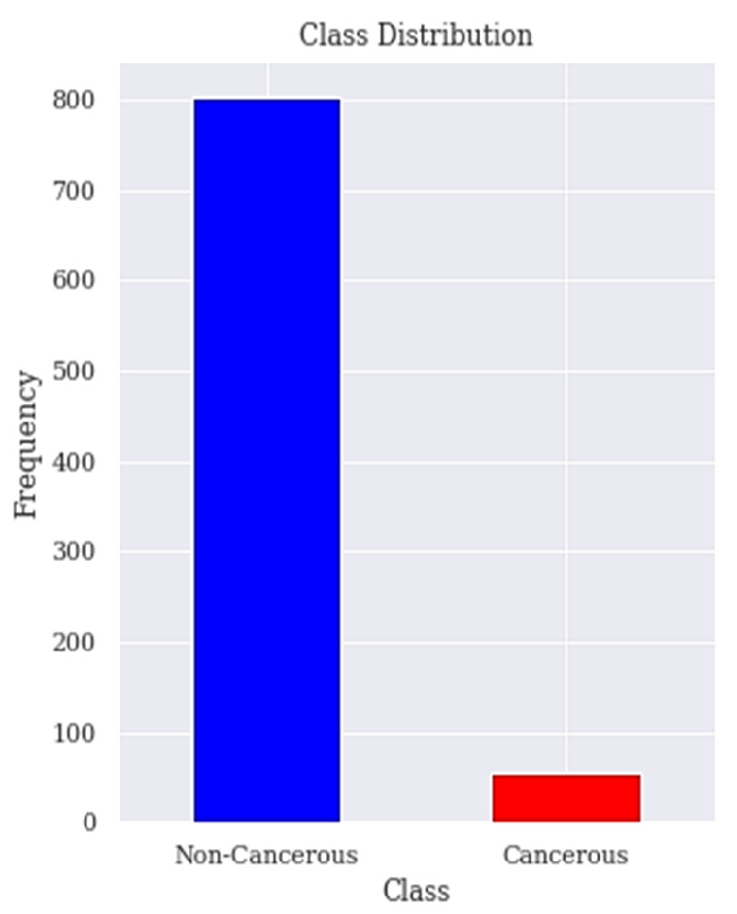
2.2. Class Imbalanced Resampling Techniques
- 4.
- Undersampling technique: A technique having a motive to maintain the distribution of the classes with the help of the removal of the majority classes randomly. Under-sampling is performed such that the number of samples of the majority class is reduced to be equal to the number of samples of the minority class [39].
- 5.
- Oversampling technique: In contrast, the data balancing can be performed by oversampling in which the new samples belonging to the minority class are generated aiming at equalizing the number of samples in both classes [39]. Over-sampling is referred to as a technique that its aim is to balance the distribution of class with the help of random replication of minority class samples. Oversampling refers to increasing the size of the minority class to balance the majority class. This method tends to duplicate the data already available or generate data on the basis of available data. The major drawback with this technique is that the synthetic samples that are created causes classifiers to create larger and less specific decision regions, rather than smaller and more specific regions [41].
- 6.
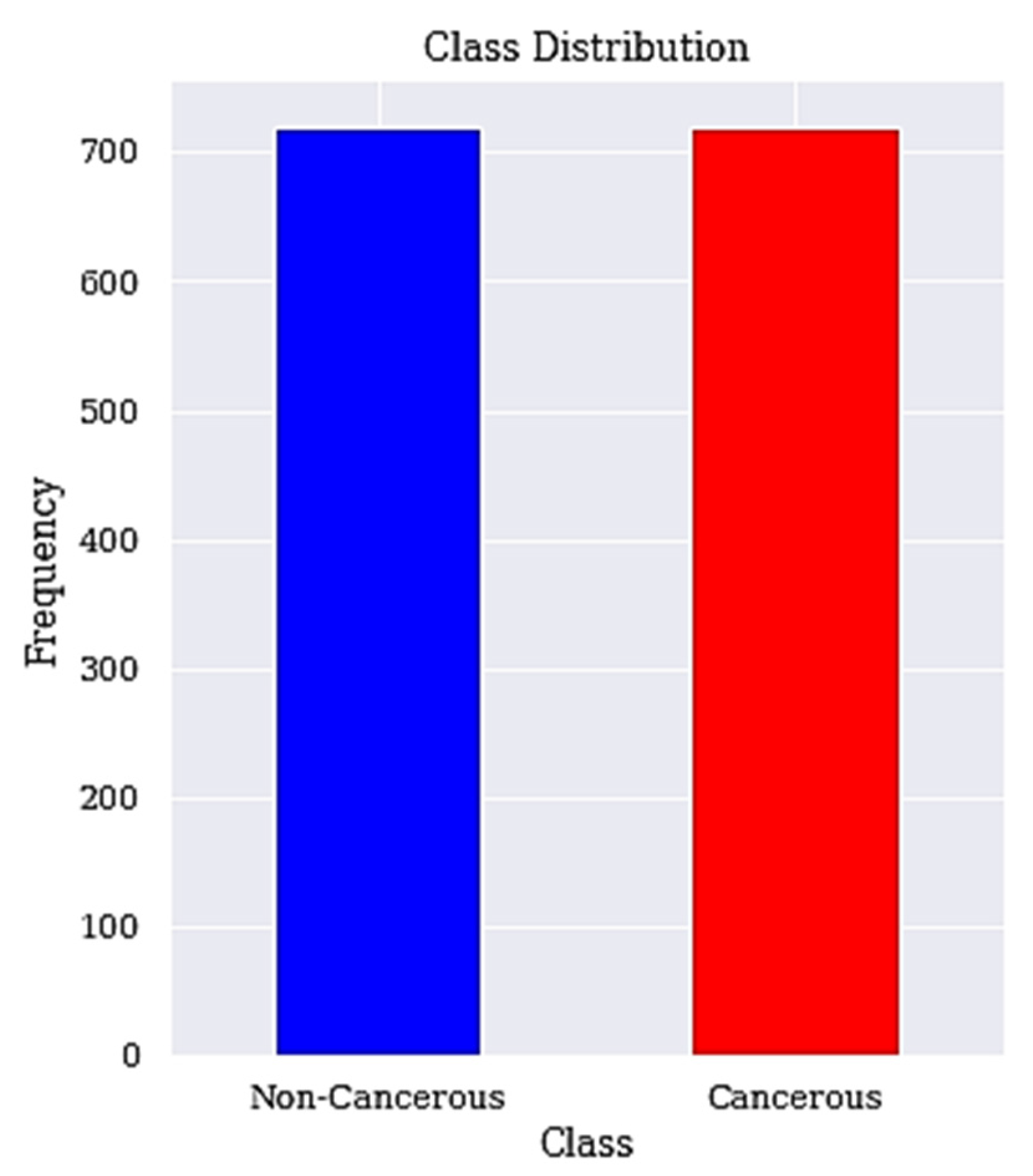
- Hybrid technique: Several studies have come up with hybrid sampling techniques that combine oversampling and under-sampling to provide a balanced dataset. One example of such technique is SMOTETomek. SMOTETomek is a hybrid approach that combines an oversampling method called the synthetic minority oversampling technique (SMOTE) with an undersampling method called Tomek. SMOTE works by taking each minority class sample and introducing synthetic samples along the line segments joining any/all of the k minority class nearest neighbors [42]. In the application of under sampling method, borderline and noise problem were detected by Tomek links. Tomek Links can be described as a method for undersampling. They can be identified as a pair of the nearest neighbors of opposite classes, which are minimally distant [43]. They are used to remove the overlapping samples that SMOTE adds [44].
2.3. Cervical Cancer Classification Techniques
2.4. Decision Trees
3. Materials and Method
3.1. Dataset Description and Visualisation
3.2. Data Preprocessing
3.3. Apply RFE Technique for Feature Selection
- Increase in model complexity and makes it difficult to interpret;
- Increase in time complexity for a model to be trained;
- Result in a bloated model with inaccurate predictions.
| Algorithm 1: Recursive Feature Elimination. |
| Step 1: Train the model using all features Step 2: Determine model’s accuracy Step 3: Determine feature’s importance to the model for each feature Step 4: for each subset Si, i = 1…N do Step 4.1: Keep the Si most important features Step 4.2: Train the model using Si features Step 4.3: Determine model’s accuracy Step 5: end for Step 6: Calculate the accuracy profile over the Si Step 7: Determine the appropriate number of features Step 8: Use the model corresponding to the optimal Si Each feature is ranked according to its importance. |
3.4. Apply LASSO Technique for Feature Selection
3.5. Resample Class Distribution Using SMOTETomek
| Algorithm 2: SMOTETomek. |
| Step 1: For a dataset D with an unbalanced data distribution, SMOTE is applied to obtain an extended dataset D’ by generating many new minority samples. Step 1.1: Let A be the minority class and let B be the majority class. Step 1.2: for each observation x belongs to class A Step 1.2.1: Identify the K-nearest neighbors of x Step 1.2.2: Randomly select few neighbors Step 1.2.3: Generate artificial observations Step 1.2.4: Spread the observations along the line joining the x to its nearest neighbors. Step 2: Tomek Link pairs in dataset D’ are removed using the Tomek Link method. Step 2.1: Let x be an instance of class A and y an instance of class B. Step 2.2: Let d(x, y) be the distance between x and y. (x, y) is a T-Link Step 2.2.1: if for any instance z, d(x, y) < d(x, z) or d(x, y) < d(y, z) Step 2.3: If any 2 samples are T-Link then one of these samples is a noise or otherwise both samples are located on the boundary of the classes. |
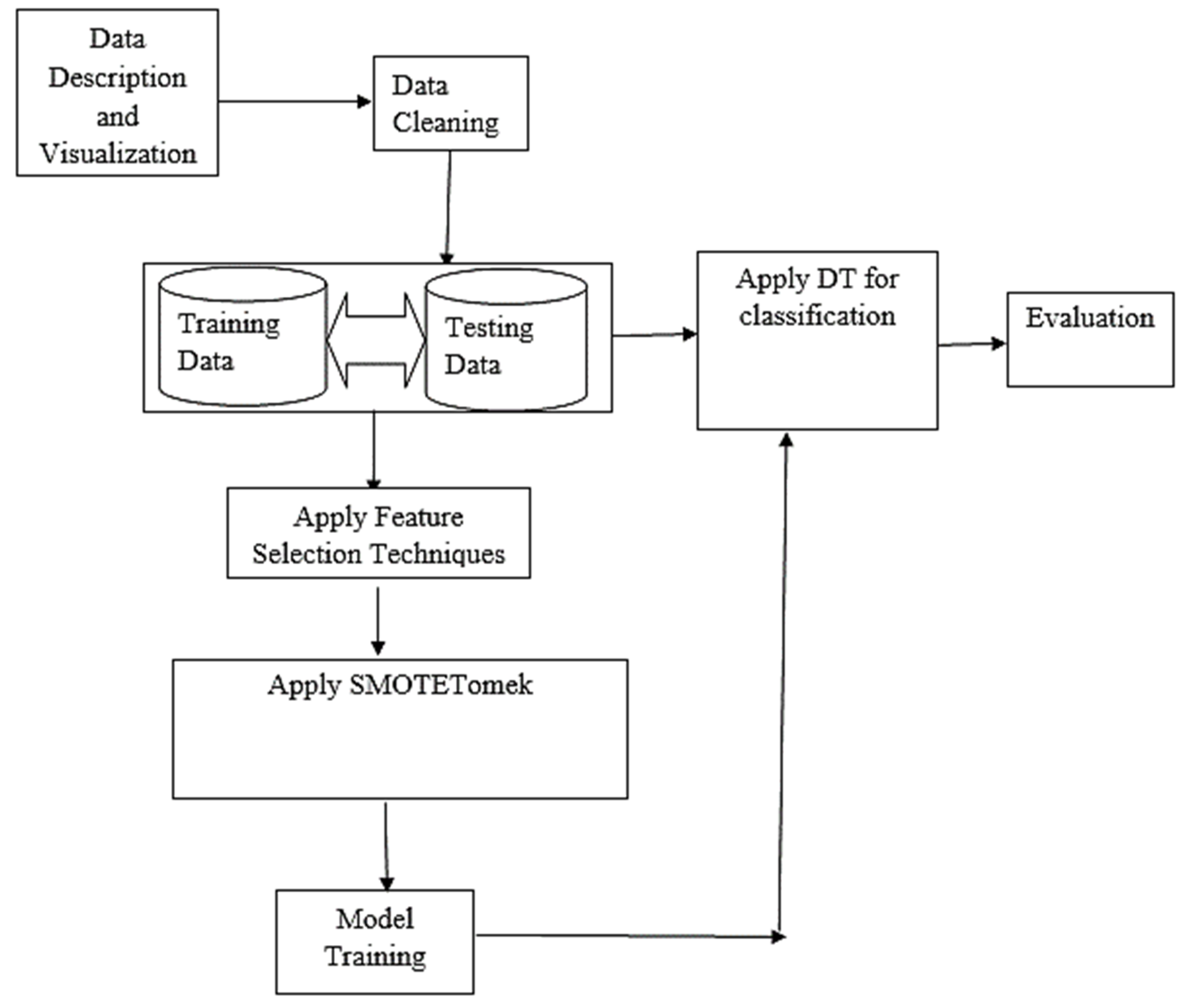
3.6. Classification
| Algorithm 3: DT Learning Algorithm. |
| Step 1: Input Dataset D = {(x1, y1), (x2, y2), ..., (xn, yn)}, Step 1.1: Attribute set A = {a1, a2, ..., am} Step 2: Function (D, A) Step 2.1: create node N Step 2.1.1: if yi = yj(∀yi, yj ∈ D) or xi = xj(∀xi, xj ∈ D) Step 2.1.2: Label (N) = mode(yi) Step 2.1.3: return Step 2.2: end if Step 2.3: choose the optimal partition attribute a* Step 2.4: for every v ∈ value(a*) Step 2.4.1: generate a new branch Dv = {xi|xi(a*) = v} Step 2.4.2: if Dv = ∅ Step 2.4.2.1: Set branch Dv as node Nv Step 2.4.2.2: Label(Nv) = mode(yi), yi ∈ D Step 2.4.3: else Step 2.4.3.1: function(Dv, A − a*) Step 2.4.4: end if Step 2.5: end for Step 3: end |
3.7. Performance Metrics
- Accuracy: The number of correct predictions by the model out the total number of predictions it is defined in Equation (3).
- 2.
- Sensitivity: The ability of the model to correctly identify people with cervical cancer. A sensitivity of 1 indicates that the model correctly predicted all the people with cervical cancer. It is defined mathematically in Equation (4).
- 3.
- Specificity: This is the metric that evaluates the model’s ability to predict people without cervical cancer. Equation (5) give the definition of specificity.
- 4.
- Precision: This metric measures the proportion of people with cervical cancer and are correctly predicted as having cervical cancer by the model. Precision measures the ratio of people with cervical cancer and are correctly predicted by the model. It is defined mathematically in Equation (6).
- 5.
- F-Measure: It is the combination of precision and sensitivity of the model and is define as the harmonic mean of the model’s precision and sensitivity. A better F-Measure means, we have a smaller number of misclassified people with or without cervical cancer. Equation (7) gives the definition of F-Measure.
- 6.
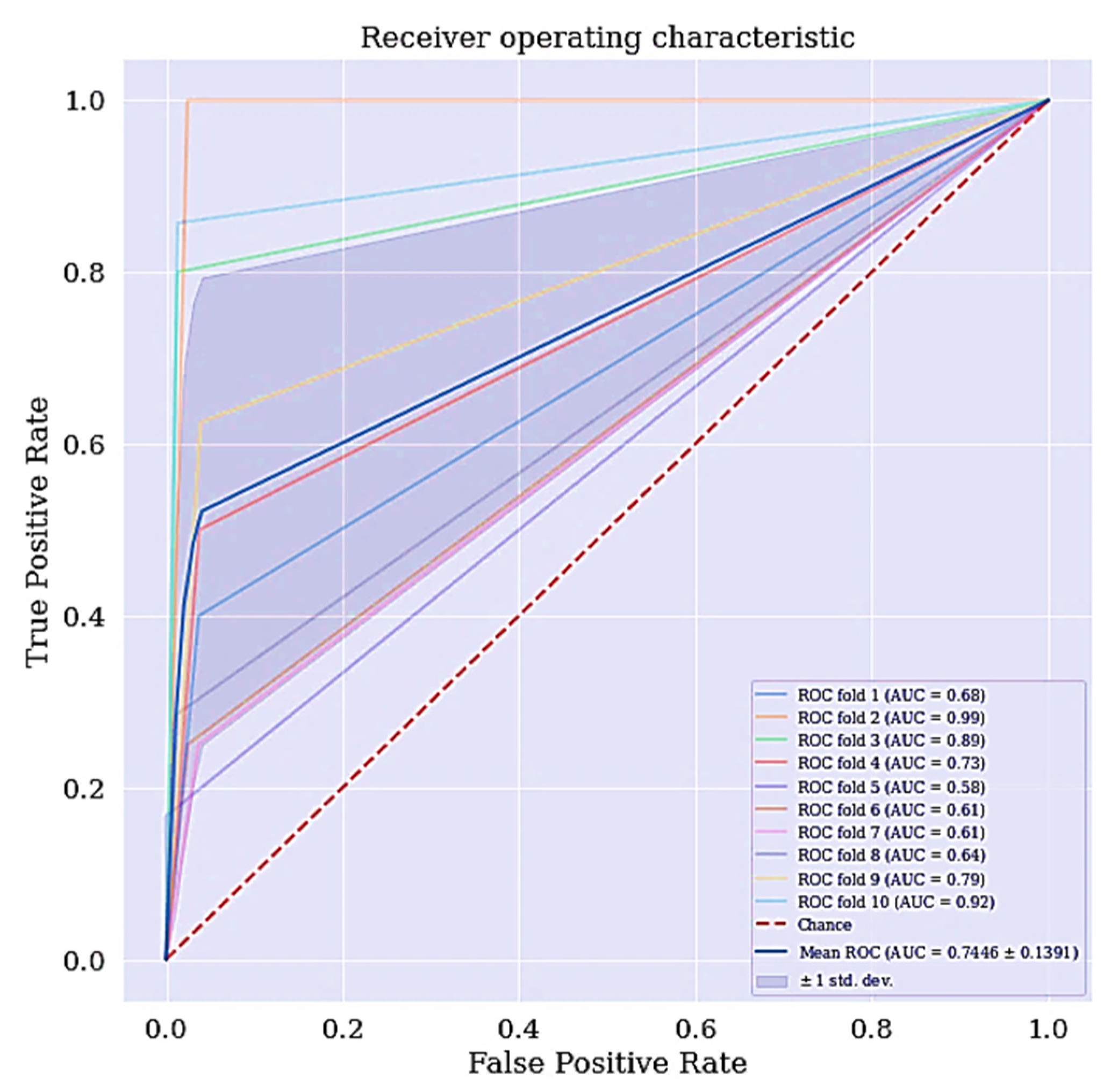
- Receiving operating characteristics curve (ROC): The ROC is a technique used for visualizing the model’s performance. It is a comprehensive index reflecting the continuous variables of sensitivity and specificity. The curve is used to define the relationship between sensitivity and specificity.
- 7.
- Area under the curve (AUC): The area under the ROC curve, abbreviated as AUC is commonly used to evaluate model’s performance. AUC measures the entire two-dimensional area under the ROC curve. The larger the AUC, the better the performance of the model.
3.8. Computational Framework
4. Results and Discussion
4.1. Basic Classification
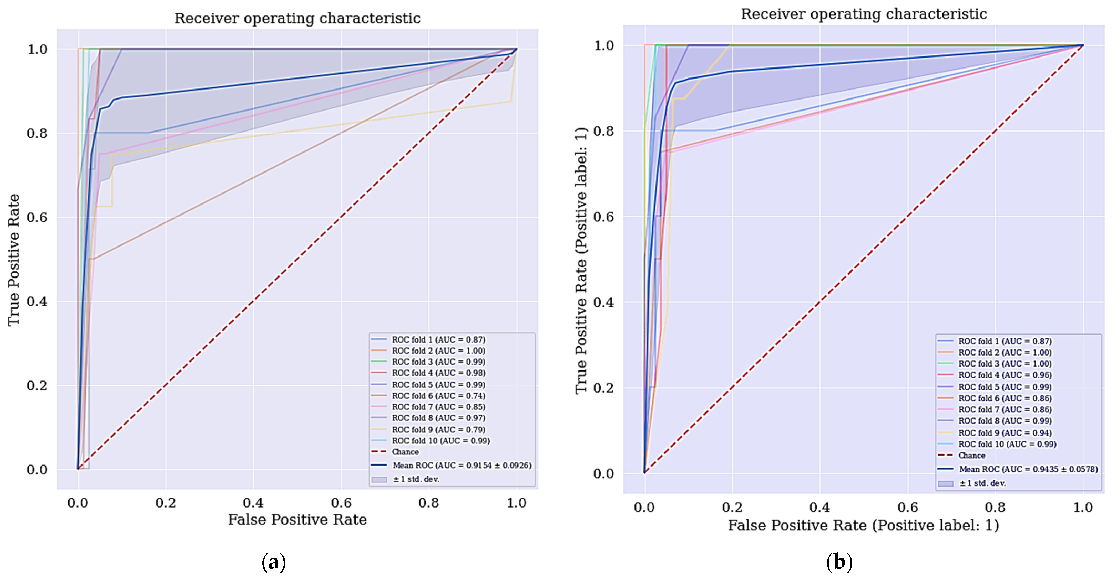
4.2. Improved Classifier with the Selected Features
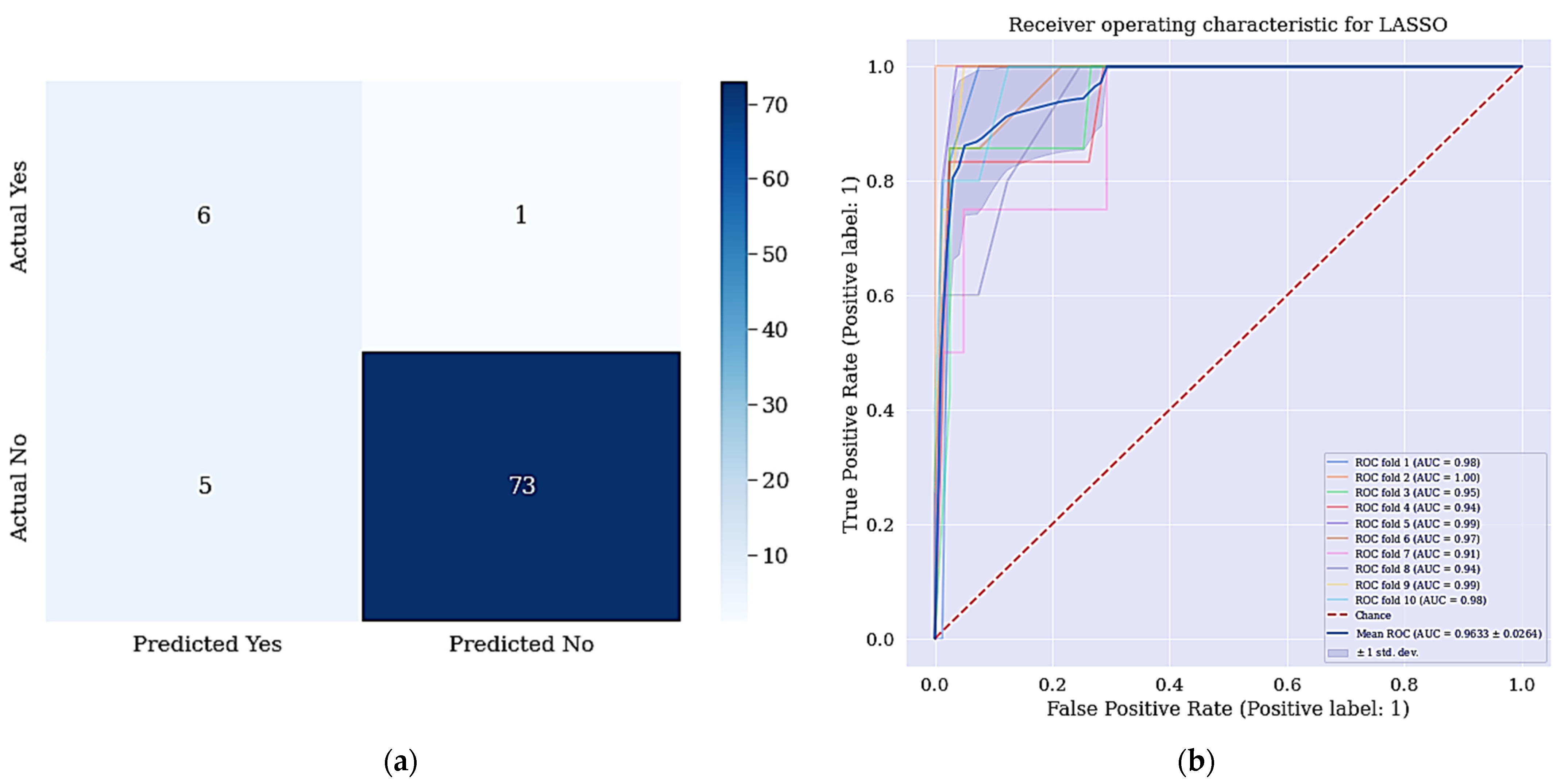
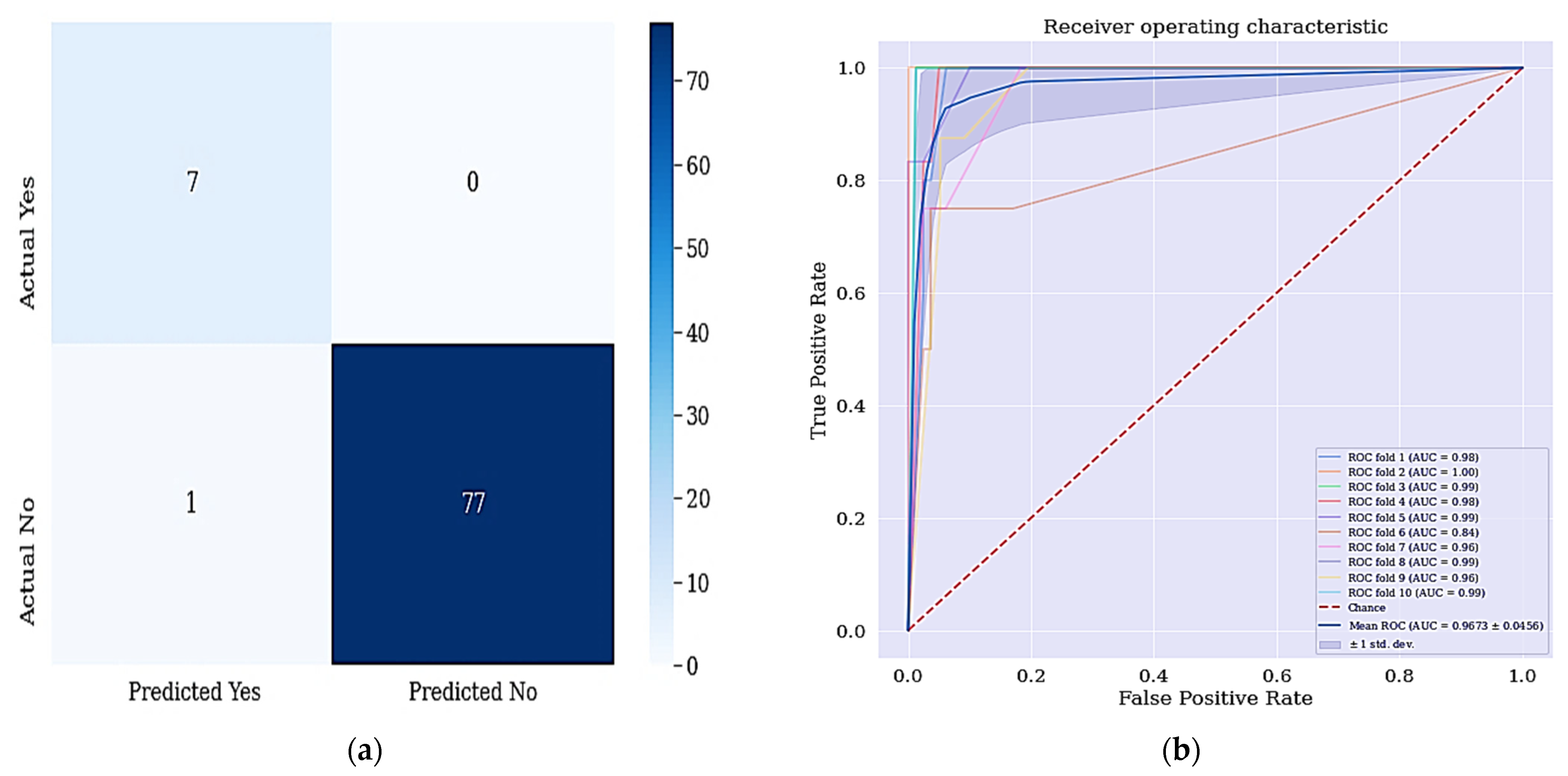
4.3. Improved Classifier with Selected Features and Resample Class Distribution
4.4. Comparison with Previous Studies
5. Conclusions
Author Contributions
Funding
Data Availability Statement
Conflicts of Interest
References
- WHO. Comprehensive Cervical Cancer Prevention and Control: A Healthier Future for Girls and Women; WHO: Geneva, Switzerland, 2013; pp. 1–12. [Google Scholar]
- Marván, M.L.; López-Vázquez, E. The Anthropocene: Politik–Economics–Society–Science: Preventing Health and Environmental Risks in Latin America; Springer: Berlin/Heidelberg, Germany, 2017. [Google Scholar]
- Ilango, B.; Nithya, V. Evaluation of machine learning based optimized feature selection approaches and classification methods for cervical cancer prediction. SN Appl. Sci. 2019, 1, 641. [Google Scholar]
- IARC. IARC-Incidencia Mundial CM; IARC: Lyon, France, 2018. [Google Scholar]
- Gunnell, A.S. Risk Factors for Cervical Cancer; Universitetsservice US-AB Nanna: Solna, Sweden, 2007. [Google Scholar]
- Castanon, A.; Sasieni, P. Is the recent increase in cervical cancer in women aged 20–24 years in England a cause for concern? Prev. Med. 2018, 107, 21–28. [Google Scholar] [CrossRef] [PubMed]
- Oluwole, E.O.; Mohammed, A.S.; Akinyinka, M.R.; Salako, O. Cervical Cancer Awareness and Screening Uptake among Rural Women in Lagos, Nigeria. J. Community Med. Prim. Health Care 2017, 29, 81–88. [Google Scholar]
- Fernandes, K.; Cardoso, J.; Fernandes, J. Automated Methods for the Decision Support of Cervical Cancer Screening Using Digital Colposcopies. IEEE Access 2018, 6, 33910–33927. [Google Scholar] [CrossRef]
- Jujjavarapu, S.E.; Deshmukh, S. Artificial Neural Network as a Classifier for the Identification of Hepato- cellular Carcinoma Through Prognosticgene Signatures. Curr. Genom. 2018, 19, 483–490. [Google Scholar] [CrossRef]
- Kourou, K.; Exarchos, T.P.; Exarchos, K.P.; Karamouzis, M.V.; Fotiadis, D.I. Machine learning applications in cancer prognosis and prediction. Comput. Struct. Biotechnol. J. 2015, 13, 8–17. [Google Scholar] [CrossRef] [Green Version]
- Singh, H.D.; Cosgrave, N. Diagnosis of Cervical Cancer Using Hybrid Machine Learning Models. Master’s Thesis, National College of Ireland, Dublin, Ireland, 2018. [Google Scholar]
- Fatlawi, H.K. Enhanced Classification Model for Cervical Cancer Dataset based on Cost Sensitive Classifier. Int. J. Comput. Tech. 2017, 4, 115–120. [Google Scholar]
- Alam, T.M.; Milhan, M.; Atif, M.; Wahab, A.; Mushtaq, M. Cervical Cancer Prediction through Different Screening Methods using Data Mining. Int. J. Adv. Comput. Sci. Appl. 2019, 10, 388–396. [Google Scholar] [CrossRef] [Green Version]
- Punjani, D.N.; Atkotiya, K.H. Cervical Cancer Test Identification Classifier using Decision Tree Method. Int. J. Res. Advent Technol. 2019, 7, 169–172. [Google Scholar] [CrossRef]
- Al-Wesabi, Y.M.S.; Choudhury, A.; Won, D. Classification of Cervical Cancer Dataset. In Proceedings of the 2018 IISE Annual Conference, Orlando, FL, USA, 19–22 May 2018; pp. 1456–1461. [Google Scholar]
- Ali, A.; Shaukat, S.; Tayyab, M.; Khan, M.A.; Khan, J.S.; Ahmad, J. Network Intrusion Detection Leveraging Machine Learning and Feature Selection. In Proceedings of the 2020 IEEE 17th International Conference on Smart Communities: Improving Quality of Life Using ICT, IoT and AI (HONET), Charlotte, NC, USA, 14–16 December 2020; pp. 49–53. [Google Scholar]
- Jessica, E.O.; Hamada, M.; Yusuf, S.I.; Hassan, M. The Role of Linear Discriminant Analysis for Accurate Prediction of Breast Cancer. In Proceedings of the 2021 IEEE 14th International Symposium on Embedded Multicore/Many-Core Systems-on-Chip (MCSoC), Singapore, 20–23 December 2021; pp. 340–344. [Google Scholar]
- Alghamdi, M.; Al-Mallah, M.; Keteyian, S.; Brawner, C.; Ehrman, J.; Sakr, S. Predicting diabetes mellitus using SMOTE and ensemble machine learning approach: The Henry Ford ExercIse Testing (FIT) project. PLoS ONE 2017, 12, e0179805. [Google Scholar] [CrossRef]
- Pang-Ning, T.; Steinbach, M.; Kumar, V. Introduction to Data Mining; Pearson Addison-Wesley: Boston, MA, USA, 2006. [Google Scholar]
- Chandrashekar, G.; Sahin, F. A survey on feature selection methods q. Comput. Electr. Eng. 2014, 40, 16–28. [Google Scholar] [CrossRef]
- Alonso-Betanzos, A. Filter Methods for Feature Selection–A Comparative Study; Springer: Berlin/Heidelberg, Germany, 2007. [Google Scholar]
- Peng, Y.; Wu, Z.; Jiang, J. A novel feature selection approach for biomedical data classification. J. Biomed. Inform. 2010, 43, 15–23. [Google Scholar] [CrossRef] [PubMed] [Green Version]
- Chen, X.; Jeong, J.C. Enhanced Recursive Feature Elimination. In Proceedings of the Sixth International Conference on Machine Learning and Applications, Cincinnati, OH, USA, 13–15 December 2007; pp. 429–435. [Google Scholar]
- Go, J.; Łukaszuk, T. Application of The Recursive Feature Elimination And The Relaxed Linear Separability Feature Selection Algorithms To Gene Expression Data Analysis. Adv. Comput. Sci. Res. 2013, 10, 39–52. [Google Scholar]
- Van Ha, S.; Nguyen, H. FRFE: Fast Recursive Feature Elimination for Credit Scoring FRFE: Fast Recursive Feature Elimination. In Proceedings of the International Conference on Nature of Computation and Communication, Rach Gia, Vietnam, 26–18 March 2016; pp. 133–142. [Google Scholar]
- Huang, S.; Cai, N.; Pacheco, P.P.; Narandes, S.; Wang, Y.; Xu, W. Applications of Support Vector Machine (SVM) Learning in Cancer Genomics. Cancer Genom.-Proteom. 2018, 15, 41–51. [Google Scholar]
- Shardlow, M. An Analysis of Feature Selection Techniques; The University of Manchester: Manchester, UK, 2016; pp. 1–7. [Google Scholar]
- Nkiama, H.; Zainudeen, S.; Saidu, M. A Subset Feature Elimination Mechanism for Intrusion Detection System. Int. J. Adv. Comput. Sci. Appl. 2016, 7, 148–157. [Google Scholar] [CrossRef]
- Ahmed, M.; Kabir, M.M.K.; Kabir, M.; Hasan, M.M. Identification of the Risk Factors of Cervical Cancer Applying Feature Selection Approaches. In Proceedings of the 3rd International Conference on Electrical, Computer & Telecommunication Engineering ICECTE 2019, Rajshahi, Bangladesh, 26–28 December 2019; pp. 201–204. [Google Scholar]
- Hamada, M.; Tanimu, J.J.; Hassan, M.; Kakudi, H.A.; Robert, P. Evaluation of Recursive Feature Elimination and LASSO Regularization-based optimized feature selection approaches for cervical cancer prediction. In Proceedings of the 2021 IEEE 14th International Symposium on Embedded Multicore/Many-Core Systems-on-Chip (MCSoC), Singapore, 20–23 December 2021; pp. 333–339. [Google Scholar]
- Rodriguez-galiano, V.F.; Luque-espinar, J.A.; Chica-olmo, M.; Mendes, M.P. Feature selection approaches for predictive modelling of groundwater nitrate pollution: An evaluation of fi lters, embedded and wrapper methods. Sci. Total Environ. 2018, 624, 661–672. [Google Scholar] [CrossRef]
- Tibshirani, R. lasso.pdf. J. R. Stat. Soc. 1996, 58, 267–288. [Google Scholar]
- Yamada, M.; Wittawat, J.; Leonid, S.; Eric, W.P.; Masashi, S. High-Dimensional Feature Selection by Feature-Wise Kernelized Lasso. Neural Comput. 2014, 207, 185–207. [Google Scholar] [CrossRef] [Green Version]
- Ghosh, P.; Azam, S.; Jonkman, M.; Karim, A.; Shamrat, F.M.J.M.; Ignatious, E.; Shultana, S.; Beeravolu, A.R.; De Boer, F. Efficient Prediction of Cardiovascular Disease Using Machine Learning Algorithms With Relief and LASSO Feature Selection Techniques. IEEE Access 2021, 9, 19304–19326. [Google Scholar] [CrossRef]
- Taylor, P.; Ludwig, N.; Feuerriegel, S.; Neumann, D. Journal of Decision Systems Putting Big Data analytics to work: Feature selection for forecasting electricity prices using the LASSO and random forests. J. Decis. Syst. 2015, 2015, 37–41. [Google Scholar]
- Zhang, H.; Wang, J.; Sun, Z.; Zurada, J.M.; Pal, N.R. Feature Selection for Neural Networks Using Group Lasso Regularization. IEEE Trans. Knowl. Data Eng. 2019, 32, 659–673. [Google Scholar] [CrossRef]
- Prati, R.C.; Batista, G.E.A.P.A.; Monard, M.C. Data mining with unbalanced class distributions: Concepts and methods. In Proceedings of the 4th Indian International Conference on Artificial Intelligence, IICAI 2009, Karnataka, India, 16–18 December 2009; pp. 359–376. [Google Scholar]
- Qiang, Y.; Xindong, W. 10 Challenging problems in data mining research. Int. J. Inf. Technol. Decis. Mak. 2006, 5, 597–604. [Google Scholar]
- Rastgoo, M.; Lemaitre, G.; Massich, J.; Morel, O.; Marzani, F.; Garcia, R.; Meriaudeau, F. Tackling the problem of data imbalancing for melanoma classification. In Proceedings of the BIOIMAGING 2016—3rd International Conference on Bioimaging, Proceedings; Part of 9th International Joint Conference on Biomedical Engineering Systems and Technologies, BIOSTEC 2016, Rome, Italy, 21–23 February 2016; pp. 32–39. [Google Scholar]
- Maheshwari, S. A Review on Class Imbalance Problem: Analysis and Potential Solutions. Int. J. Comput. Sci. Issues 2017, 14, 43–51. [Google Scholar]
- Somasundaram, A.; Reddy, U.S. Data Imbalance: Effects and Solutions for Classification of Large and Highly Imbalanced Data. In Proceedings of the 1st International Conference on Research in Engineering, Computers, and Technology (ICRECT 2016), Tiruchirappalli, India, 8–10 September 2016; pp. 28–34. [Google Scholar]
- Cengiz Colak, M.; Karaaslan, E.; Colak, C.; Arslan, A.K.; Erdil, N. Handling imbalanced class problem for the prediction of atrial fibrillation in obese patient. Biomed. Res. 2017, 28, 3293–3299. [Google Scholar]
- Yan, Y.; Liu, R.; Ding, Z.; Du, X.; Chen, J.; Zhang, Y. A parameter-free cleaning method for SMOTE in imbalanced classification. IEEE Access 2019, 7, 23537–23548. [Google Scholar] [CrossRef]
- Wang, Z.H.E.; Wu, C.; Zheng, K.; Niu, X.; Wang, X. SMOTETomek-based Resampling for Personality Recognition. IEEE Access 2019, 7, 129678–129689. [Google Scholar] [CrossRef]
- More, A. Survey of resampling techniques for improving classification performance in unbalanced datasets. arXiv 2016, arXiv:1608.06048. [Google Scholar]
- Goel, G.; Maguire, L.; Li, Y.; McLoone, S. Evaluation of Sampling Methods for Learning from Imbalanced Data. In Intelligent Computing Theories; Springer: Berlin/Heidelberg, Germany, 2013; pp. 392–401. [Google Scholar]
- Chen, T.; Shi, X.; Wong, Y.D. Key feature selection and risk prediction for lane-changing behaviors based on vehicles’ trajectory data. Accid. Anal. Prev. 2019, 129, 156–169. [Google Scholar] [CrossRef]
- Le, T.; Baik, S.W. A Robust Framework for Self-Care Problem Identification for Children with Disability. Symmetry 2019, 11, 89. [Google Scholar] [CrossRef] [Green Version]
- Teixeira, V.; Camacho, R.; Ferreira, P.G. Learning influential genes on cancer gene expression data with stacked denoising autoencoders. In Proceedings of the 2017 IEEE International Conference on Bioinformatics and Biomedicine (BIBM), Kansas City, MO, USA, 23–16 November 2017; pp. 1201–1205. [Google Scholar]
- Fitriyani, N.L.; Syafrudin, M.; Alfian, G.; Rhee, J. Development of Disease Prediction Model Based on Ensemble Learning Approach for Diabetes and Hypertension. IEEE Access 2019, 7, 144777–144789. [Google Scholar] [CrossRef]
- Zeng, M.; Zou, B.; Wei, F.; Liu, X.; Wang, L. Effective prediction of threecommondiseases by combining SMOTE with Tomek links technique for imbalanced medical data. In Proceedings of the 2016 IEEE International Conference of Online Analysis and Computing Science (ICOACS), Chongqing, China, 28–29 May 2016; pp. 225–228. [Google Scholar]
- William, W.; Ware, A.; Basaza-ejiri, A.H.; Obungoloch, J. A review of image analysis and machine learning techniques for automated cervical cancer screening from pap-smear images. Comput. Methods Programs Biomed. 2018, 164, 15–22. [Google Scholar] [CrossRef]
- Fernandes, K.; Cardoso, J.S.; Fernandes, J. Transfer learning with partial observability applied to cervical cancer screening. In Proceedings of the Iberian Conference on Pattern Recognition and Image Analysis, Faro, Portugal, 20–23 June 2017; Springer: Cham, Switzerland, 2017; pp. 243–250. [Google Scholar]
- Wu, W.; Zhou, H. Data-Driven Diagnosis of Cervical Cancer With Support Vector Machine-Based Approaches. IEEE Access 2017, 5, 25189–25195. [Google Scholar] [CrossRef]
- Shah, J.H.; Sharif, M.; Yasmin, M.; Fernandes, S.L. Facial expressions classification and false label reduction using LDA and threefold SVM. Pattern Recognit. Lett. 2017, 139, 166–173. [Google Scholar] [CrossRef]
- Karamizadeh, S.; Abdullah, S.M.; Halimi, M.; Shayan, J.; Rajabi, M.J. Advantage and drawback of support vector machine functionality. In Proceedings of the I4CT 2014-1st International Conference on Computer, Communications, and Control Technology, Kedah, Malaysia, 2–4 September 2014; pp. 63–65. [Google Scholar]
- Raschka, S. Model Evaluation, Model Selection, and Algorithm Selection in Machine Learning. arXiv 2020, arXiv:1811.12808. [Google Scholar]
- Yadav, S. Analysis of k-fold cross-validation over hold-out validation on colossal datasets for quality classification. In Proceedings of the 2016 IEEE 6th International Conference on Advanced Computing (IACC), Bhimavaram, India, 27–28 February 2016. [Google Scholar]
- Abdoh, S.F.; Rizka, M.A.; Maghraby, F.A. Cervical Cancer Diagnosis Using Random Forest Classifier With SMOTE and Feature Reduction Techniques. IEEE Access 2018, 6, 59475–59485. [Google Scholar] [CrossRef]
- Deng, X.; Luo, T.; Wang, C. Analysis of Risk Factors for Cervical Cancer Based on Machine Learning Methods. In Proceedings of the 2018 5th IEEE International Conference on Cloud Computing and Intelligence Systems (CCIS), Nanjing, China, 23–25 November 2018; pp. 631–635. [Google Scholar]
- Alsmariy, R.; Healy, G.; Abdelhafez, H. Predicting Cervical Cancer using Machine Learning Methods. Int. J. Adv. Comput. Sci. Appl. 2020, 11, 173–184. [Google Scholar] [CrossRef]
- Ghoneim, A.; Muhammad, G.; Hossain, S.M. Machine learning for assisting cervical cancer diagnosis: An ensemble approach, Futur. Gener. Comput. Syst. 2020, 106, 199–205. [Google Scholar]
- Ghoneim, A.; Muhammad, G.; Hossain, M.S. Cervical cancer classification using convolutional neural networks and extreme learning machines. Future Gener. Comput. Syst. 2019, 102, 643–649. [Google Scholar] [CrossRef]
- Musa, A.; Hamada, M.; Aliyu, F.M.; Hassan, M. An Intelligent Plant Dissease Detection System for Smart Hydroponic using Convolutional Neural Network. In Proceedings of the 2021 IEEE 14th International Symposium on Embedded Multicore/Many-Core Systems-on-Chip (MCSoC), Singapore, 20–23 December 2021; pp. 345–351. [Google Scholar]
- Sepandi, M.; Taghdir, M.; Rezaianzadeh, A.; Rahimikazerooni, S. Assessing Breast Cancer Risk with an Artificial Neural Network. Asian Pac. J. Cancer Prev. 2018, 19, 1017–1019. [Google Scholar]
- Ayer, T.; Alagoz, O.; Chhatwal, J.; Shavlik, J.W.; Kahn, C.; Burnside, E.S. Breast cancer risk estimation with artificial neural networks revisited. Cancer 2010, 116, 3310–3321. [Google Scholar] [CrossRef] [Green Version]
- Yamashita, R.; Nishio, M.; Do, R.K.G.; Togashi, K. Convolutional neural networks: An overview and application in radiology. Insights Imaging 2018, 9, 611–629. [Google Scholar] [CrossRef] [Green Version]
- Ijaz, M.F.; Attique, M.; Son, Y. Data-Driven Cervical Cancer Prediction Model with Outlier Detection and Over-Sampling Methods. Sensors 2020, 20, 2809. [Google Scholar] [CrossRef]
- Saxena, R. Building Decision Tree Algorithm in Python with Decision Tree Algorithm Implementation with Scikit Learn How We Can Implement Decision Tree Classifier. 2018, pp. 1–16. Available online: https://dataaspirant.com/decision-tree-algorithm-python-with-scikit-learn/ (accessed on 1 February 2017).
- Jujjavarapu, S.; Chandrakar, N. Artificial neural networks as classification and diagnostic tools for lymph node-negative breast cancers. Korean J. Chem. Eng. 2016, 33, 1318–1324. [Google Scholar]
- De Ville, B. Decision Trees for Business Intelligence and Data Mining: Using SAS Enterprise Miner. Lect. Notes Math. 2008, 1928, 67–86. [Google Scholar]
- Shekar, B.H.; Dagnew, G. Grid Search-Based Hyperparameter Tuning and Classification of Microarray Cancer Data. In Proceedings of the Second International Conference on Advanced Computational and Communication Paradigms (ICACCP-2019), Gangtok, India, 25–28 February 2019. [Google Scholar]
- Tabares-Soto, R.; Orozco-Arias, S.; Romero-Cano, V.; Bucheli, V.S.; Rodríguez-Sotelo, J.L.; Jiménez-Varón, C.F. A comparative study of machine learning and deep learning algorithms to classify cancer types based on microarray gene expression data. PeerJ Comput. Sci. 2020, 6, e270. [Google Scholar] [CrossRef] [PubMed] [Green Version]
- Bramer, M. Principles of Data Mining; Springer: Berlin/Heidelberg, Germany, 2007. [Google Scholar]
- Kerdprasop, N. Discrete Decision Tree Induction to Avoid Overfitting on Categorical Data. In Proceedings of the MAMECTIS/NOLASC/CONTROL/WAMUS’11, Iasi, Romania, 1–3 July 2011. [Google Scholar]
- Patel, R.; Aluvalu, R. A Reduced Error Pruning Technique for Improving Accuracy of Decision Tree Learning. Int. J. Adv. Sci. Eng. Inf. Technol. 2014, 3, 8–11. [Google Scholar]
- Patil, D.D.; Wadhai, V.; Gokhale, J. Evaluation of Decision Tree Pruning Algorithms for Complexity and Classification Accuracy. Int. J. Comput. Appl. 2010, 11, 23–30. [Google Scholar] [CrossRef]
- Berrar, D. Cross-Validation. In Reference Module in Life Sciences; Elsevier: Amsterdam, The Netherlands, 2019. [Google Scholar]
- Hassan, M. Smart Media-based Context-aware Recommender Systems for Learning: A Conceptual Framework. In Proceedings of the 16th International Conference on Information Technology Based Higher Education and Training (ITHET), Ohrid, Macedonia, 10–12 June 2017. [Google Scholar]
- Hassan, M. A Fuzzy-based Approach for Modelling Preferences of Users in Multi-criteria Recommender Systems. In Proceedings of the 2018 IEEE 12th International Symposium on Embedded Multicore/Many-Core Systems-on-Chip (MCSoC), Hanoi, Vietnam, 12–14 September 2018. [Google Scholar]
- Tanimu, J.J.; Hamada, M.; Hassan, M.; Yusuf, S.I. A Contemporary Machine Learning Method for Accurate Prediction of Cervical Cancer. In Proceedings of the 3rd ETLTC2021-ACM International Conference om Information and Communications Technology, Aizu, Japan, 27–30 January 2021; p. 04004. [Google Scholar]


| S/N | Features | Data Types |
|---|---|---|
| 1 | Age | Integer |
| 2 | Number of sexual partners | Integer |
| 3 | First sexual intercourse (age) | Integer |
| 4 | Number of pregnancies | Integer |
| 5 | Smokes | Boolean |
| 6 | Smokes (years) | Integer |
| 7 | Smokes (packs/year) | Integer |
| 8 | Hormonal contraceptives | Boolean |
| 9 | Hormonal contraceptives (years) | Integer |
| 10 | IUD | Boolean |
| 11 | IUD (years) | Integer |
| 12 | STDs | Boolean |
| 13 | STDs (number) | Integer |
| 14 | STDS: Condylomatosis | Boolean |
| 15 | STDS: Cervical condylomatosis | Boolean |
| 16 | STDS: Cervical condylomatosis | Boolean |
| 17 | STDS: Vulvo-perineal condylomatosis | Boolean |
| 18 | STDS: Syphilis | Boolean |
| 19 | STDS: Pelvic inflammatory disease | Boolean |
| 20 | STDS: Genital herpes | Boolean |
| 21 | STDS: Molluscum cotagiosum | Boolean |
| 22 | STDS: AIDS | Boolean |
| 23 | STDS: HIV | Boolean |
| 24 | STDS: Hepatits B | Boolean |
| 25 | STDS: HPV | Boolean |
| 26 | STDS: Number of diagnoses | Integer |
| 27 | STDS: Time since first diagnosis | Integer |
| 28 | STDS: Time since last diagnosis | Integer |
| 29 | Dx: Cancer | Boolean |
| 30 | Dx: CIN | Boolean |
| 31 | Dx: HPV | Boolean |
| 32 | Dx: | Boolean |
| 33 | Hinselmann | Boolean |
| 34 | Schiller | Boolean |
| 35 | Cytology | Boolean |
| 36 | Biopsy (Target) | Boolean |
| Evaluation Metrics | DT Performance |
|---|---|
| Accuracy | 95.29% |
| Sensitivity | 85.71% |
| Specificity | 96.15% |
| Precision | 66.67% |
| F-measure | 75.01% |
| AUC | 74.46% |
| SN | Features |
|---|---|
| 1 | Age |
| 2 | Dx: |
| 3 | Dx: CIN |
| 4 | Dx: Cancer |
| 5 | STDs: Number of diagnoses |
| 6 | STDs: HPV |
| 7 | STDs: Hepatitis B |
| 8 | STDs: HIV |
| 9 | STDs: AIDS |
| 10 | STDs: Molluscum contagiosum |
| 11 | Hormonal contraceptives (years) |
| 12 | Number of sexual partners |
| 13 | First sexual intercourse |
| 14 | STDs |
| 15 | IUD (years) |
| 16 | IUD |
| 17 | Hormonal contraceptives |
| 18 | Smokes (packs/year) |
| 19 | Smokes |
| 20 | Number of pregnancies |
| Features | LASSO Coefficients |
|---|---|
| Age | −2.912 |
| Number of sexual partners | −4.133 |
| First sexual intercourse (age) | −6.216 |
| Smokes (years) | −2.697 |
| Smokes (packs/year) | 1.858 |
| Hormonal contraceptives (years) | 5.706 |
| STDs | 1.802 |
| STDS: Syphilis | −8.344 |
| Dx: CIN | 2.473 |
| Dx: | 2.875 |
| Evaluation Metrics | DT | DT + RFE | DT + LASSO |
|---|---|---|---|
| Accuracy | 95.29% | 97.65% | 96.47% |
| Sensitivity | 85.71% | 85.71% | 71.43% |
| Specificity | 96.15% | 98.72% | 98.71% |
| Precision | 66.67% | 85.71% | 83.33% |
| F-Measure | 75.01% | 85.71% | 76.92% |
| AUC | 74.46% | 91.54% | 94.35% |
| Evaluation Metrics | DT + RFE + SMOTETomek | DT + LASSO + SMOTETomek |
|---|---|---|
| Accuracy | 98.82% | 92.94% |
| Sensitivity | 100% | 85.71% |
| Specificity | 98.71% | 93.59% |
| Precision | 87.51% | 54.55% |
| F-Measure | 93.33% | 66.67% |
| AUC | 96.73% | 96.33% |
| Studies | Method | No. of Features | Accuracy | Sensitivity | Specificity |
|---|---|---|---|---|---|
| Abdoh et al. [59] | SMOTE-RF | 30 | 96.06% | 94.55% | 97.51% |
| SMOTE-RF-RFE | 18 | 95.87% | 94.42% | 97.26% | |
| SMOTE-RF-PCA | 11 | 95.74% | 94.16% | 97.76% | |
| Ijaz et al. [68] | DBSCAN + SMOTETomek + RF | 10 | 97.72% | 97.43% | 98.01% |
| DBSCAN + SMOTE+ RF | 10 | 97.22% | 96.43% | 98.01% | |
| iForest + SMOTETomek + RF | 10 | 97.50% | 97.91% | 97.08% | |
| iForest + SMOTE + RF | 10 | 97.58% | 97.45% | 97.58% | |
| Present Studies | RFE + DT | 20 | 97.65% | 85.71% | 98.72% |
| LASSO + DT | 10 | 96.47% | 71.43% | 98.71% | |
| RFE + SMOTETomek + DT | 20 | 98.82% | 100% | 98.71% | |
| LASSO + SMOTETomek + DT | 10 | 92.94% | 85.71% | 93.59% |
Publisher’s Note: MDPI stays neutral with regard to jurisdictional claims in published maps and institutional affiliations. |
© 2022 by the authors. Licensee MDPI, Basel, Switzerland. This article is an open access article distributed under the terms and conditions of the Creative Commons Attribution (CC BY) license (https://creativecommons.org/licenses/by/4.0/).
Share and Cite
Tanimu, J.J.; Hamada, M.; Hassan, M.; Kakudi, H.; Abiodun, J.O. A Machine Learning Method for Classification of Cervical Cancer. Electronics 2022, 11, 463. https://doi.org/10.3390/electronics11030463
Tanimu JJ, Hamada M, Hassan M, Kakudi H, Abiodun JO. A Machine Learning Method for Classification of Cervical Cancer. Electronics. 2022; 11(3):463. https://doi.org/10.3390/electronics11030463
Chicago/Turabian StyleTanimu, Jesse Jeremiah, Mohamed Hamada, Mohammed Hassan, Habeebah Kakudi, and John Oladunjoye Abiodun. 2022. "A Machine Learning Method for Classification of Cervical Cancer" Electronics 11, no. 3: 463. https://doi.org/10.3390/electronics11030463
APA StyleTanimu, J. J., Hamada, M., Hassan, M., Kakudi, H., & Abiodun, J. O. (2022). A Machine Learning Method for Classification of Cervical Cancer. Electronics, 11(3), 463. https://doi.org/10.3390/electronics11030463