
Accurate Photovoltaic Models Based on an Adaptive Opposition Artificial Hummingbird Algorithm


 ,
,  ,
,  and
and 
Abstract
:1. Introduction
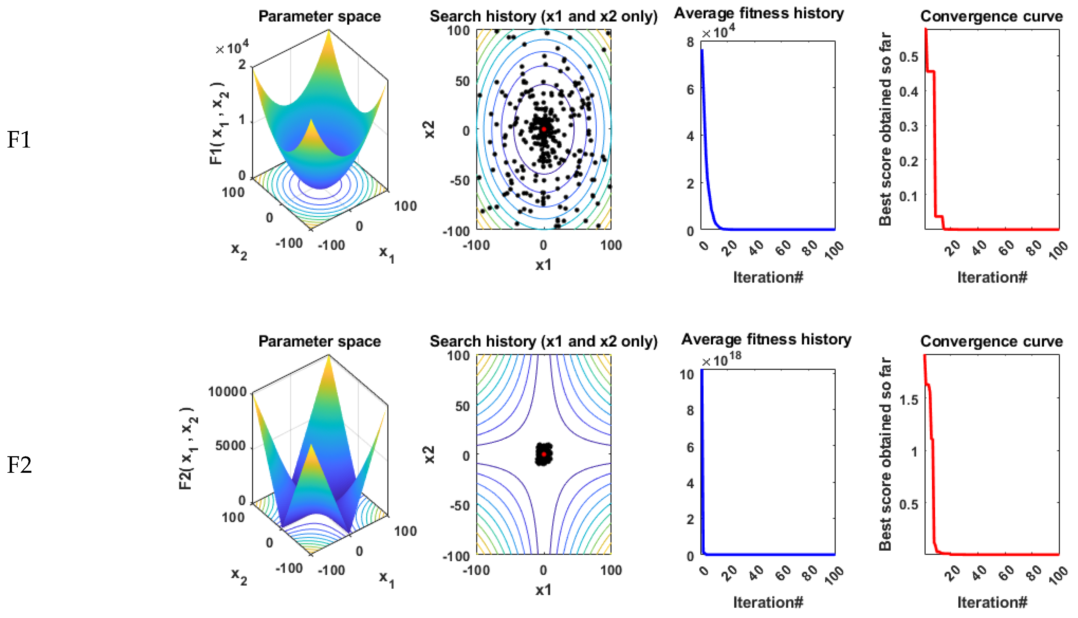
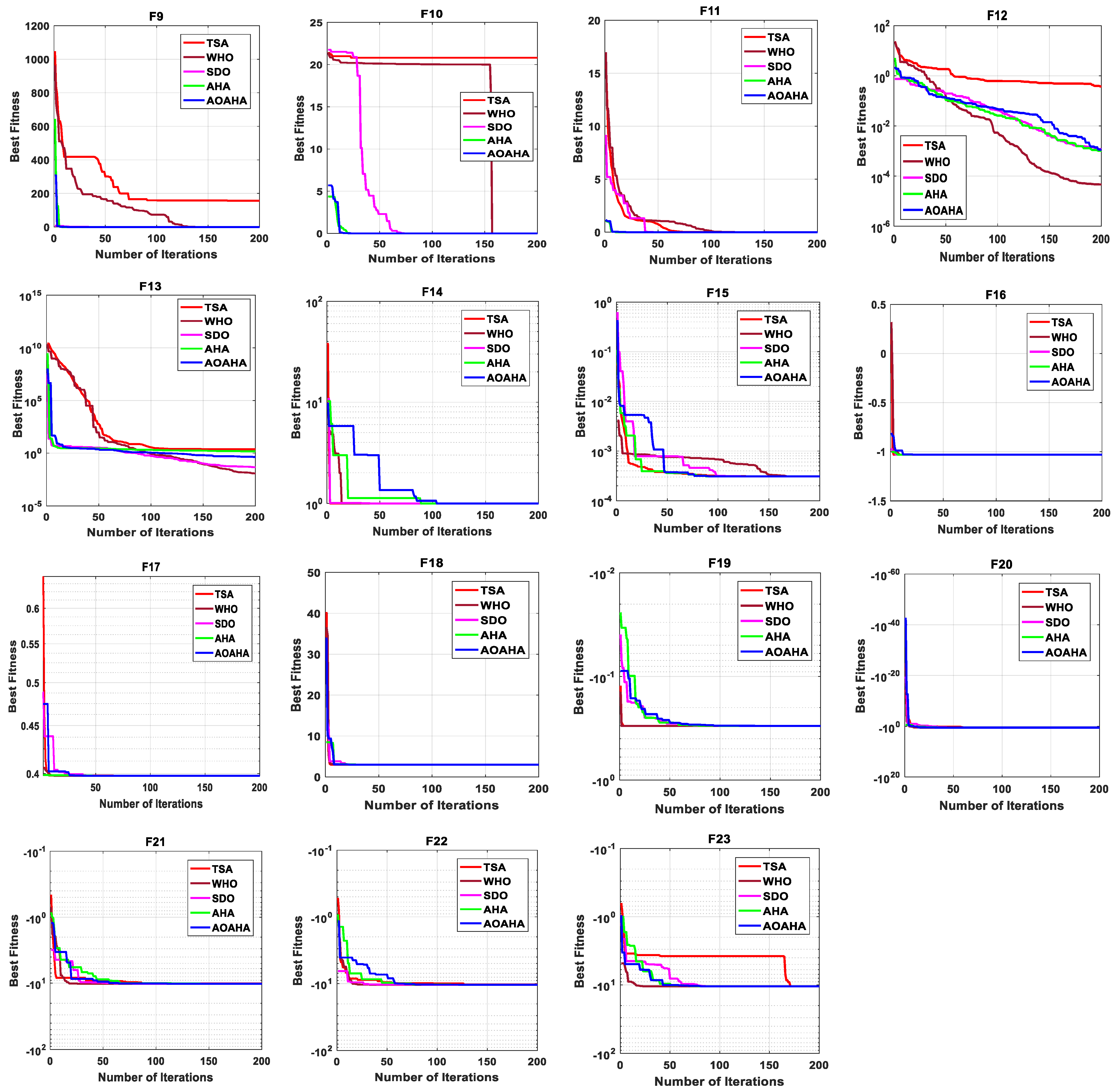
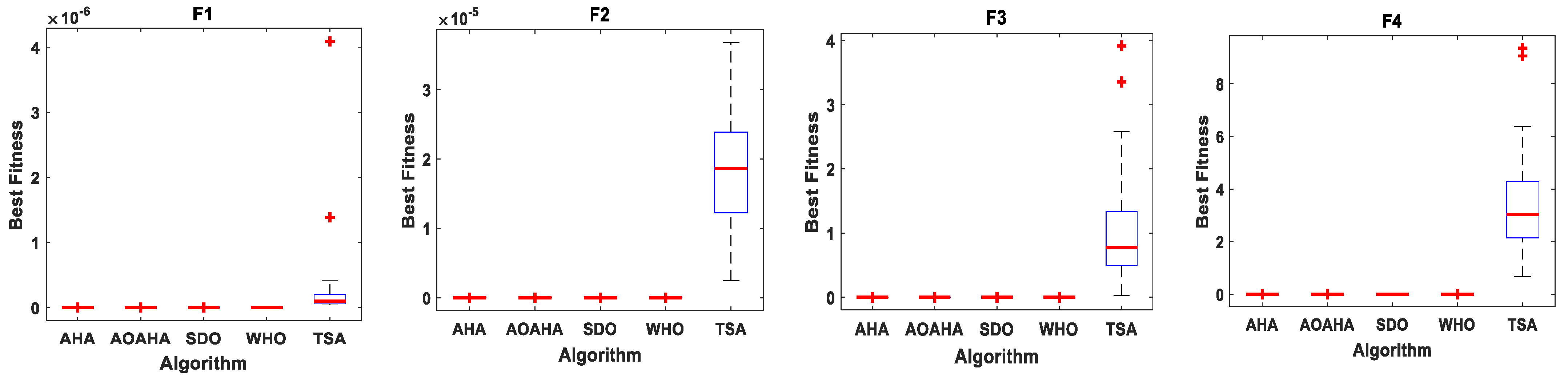
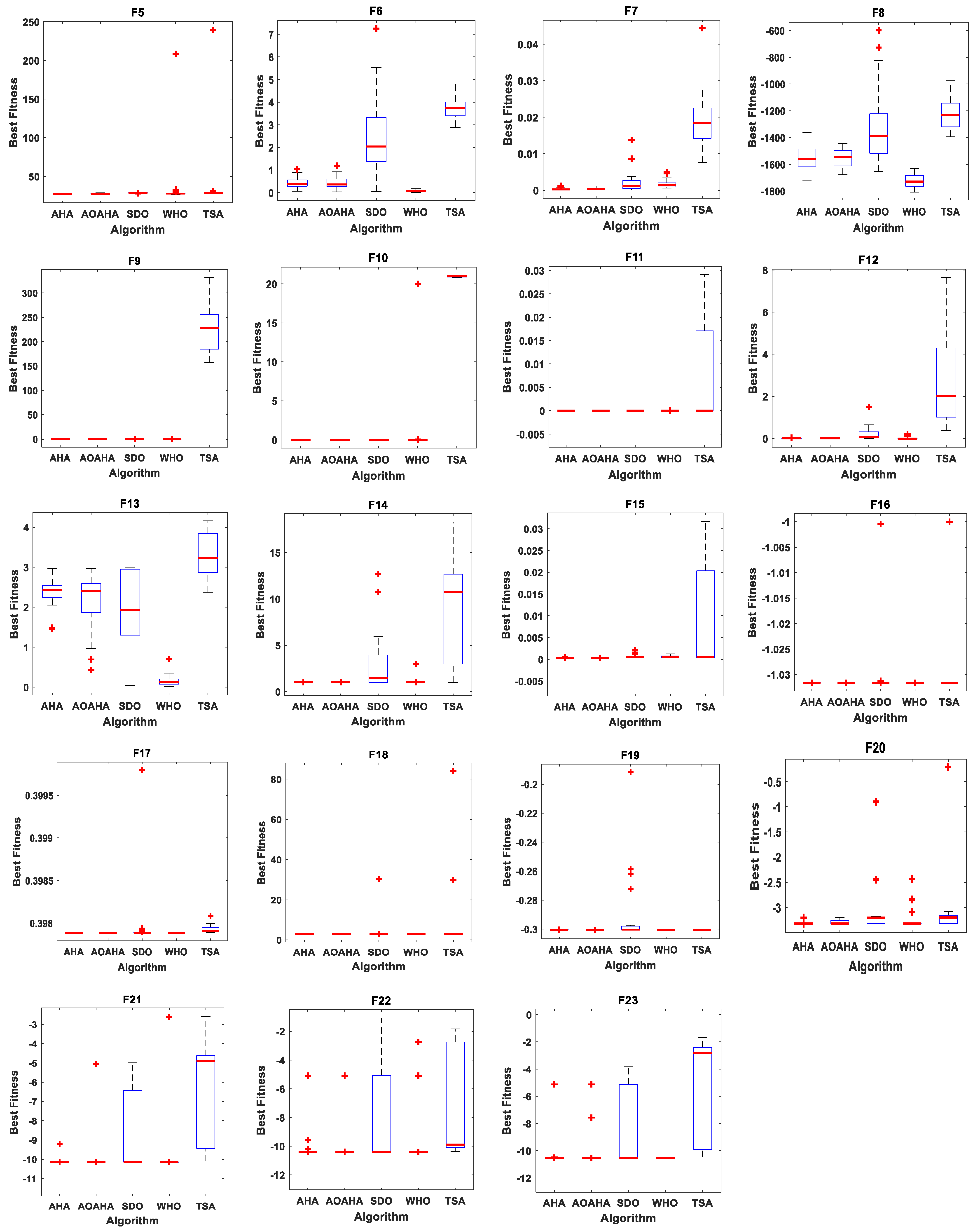
- A novel enhanced algorithm (AOAHA) has been proposed and tested through unimodal, multimodal, and composite benchmark functions, totaling 23 benchmark functions;
- The enhancement was based on an adaptive opposition approach that suggests whether or not to use an opposition-based learning (OBL) method;
- AOAHA was applied to estimate accurate PV models with consideration of a complex optimization problem, due to the nonlinearities in the PV system’s behavior;
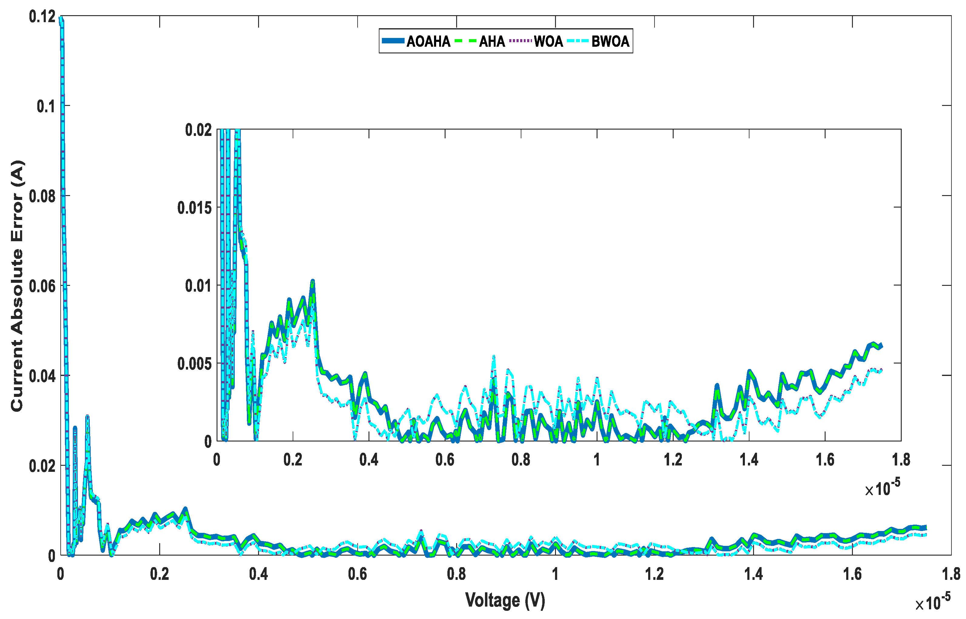
- The estimated models and the algorithm behavior were evaluated through different evaluation methods, such as RMSE, absolute error statistical analysis, and algorithm convergence curves;
- The proposed algorithm gives better results than the original and other recent algorithms, both in the benchmark functions and in the real PV application. The enhancement approach increased the exploration and exploitation balance of the original algorithm, as well as its probability of avoiding local optima problems.
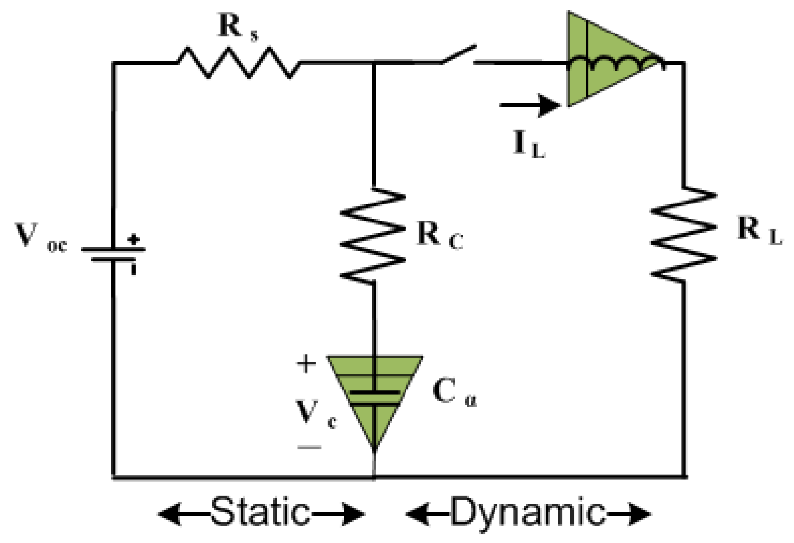
2. PV Models (Static and Dynamic)
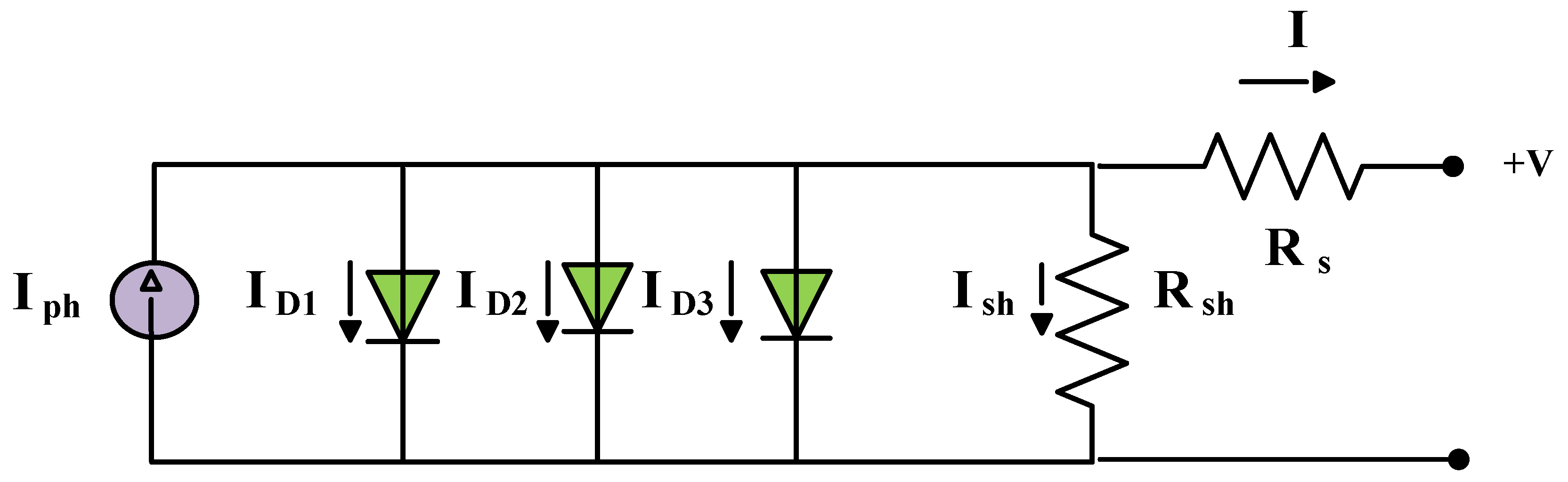
2.1. Static TDM
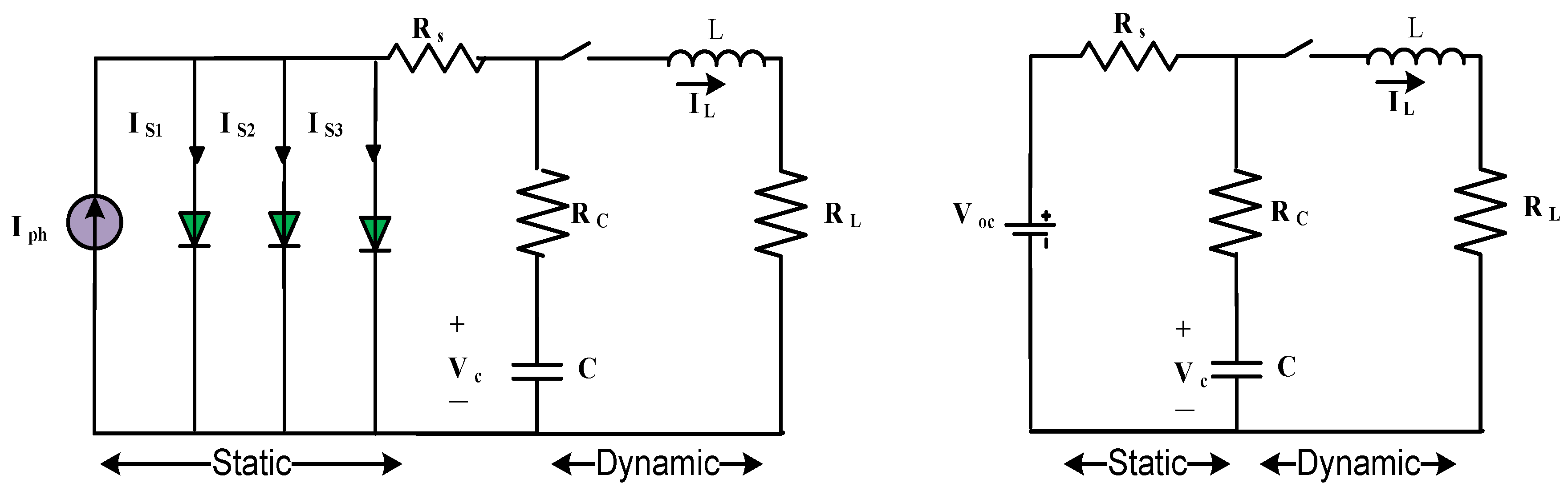
2.2. Dynamic PV Model
- -
- : Constant voltage source (static part);
- -
- : Series resistance to represent the static model (static part);
- -
- : Capacitor for junction capacitance (dynamic part);
- -
- : Resistance for conductance (dynamic part);
- -
- : The connected cables’ inductance is represented by the coil inductance (dynamic part);
- -
- : Resistance to represent the load (dynamic part).
3. The Proposed Optimization Methodology
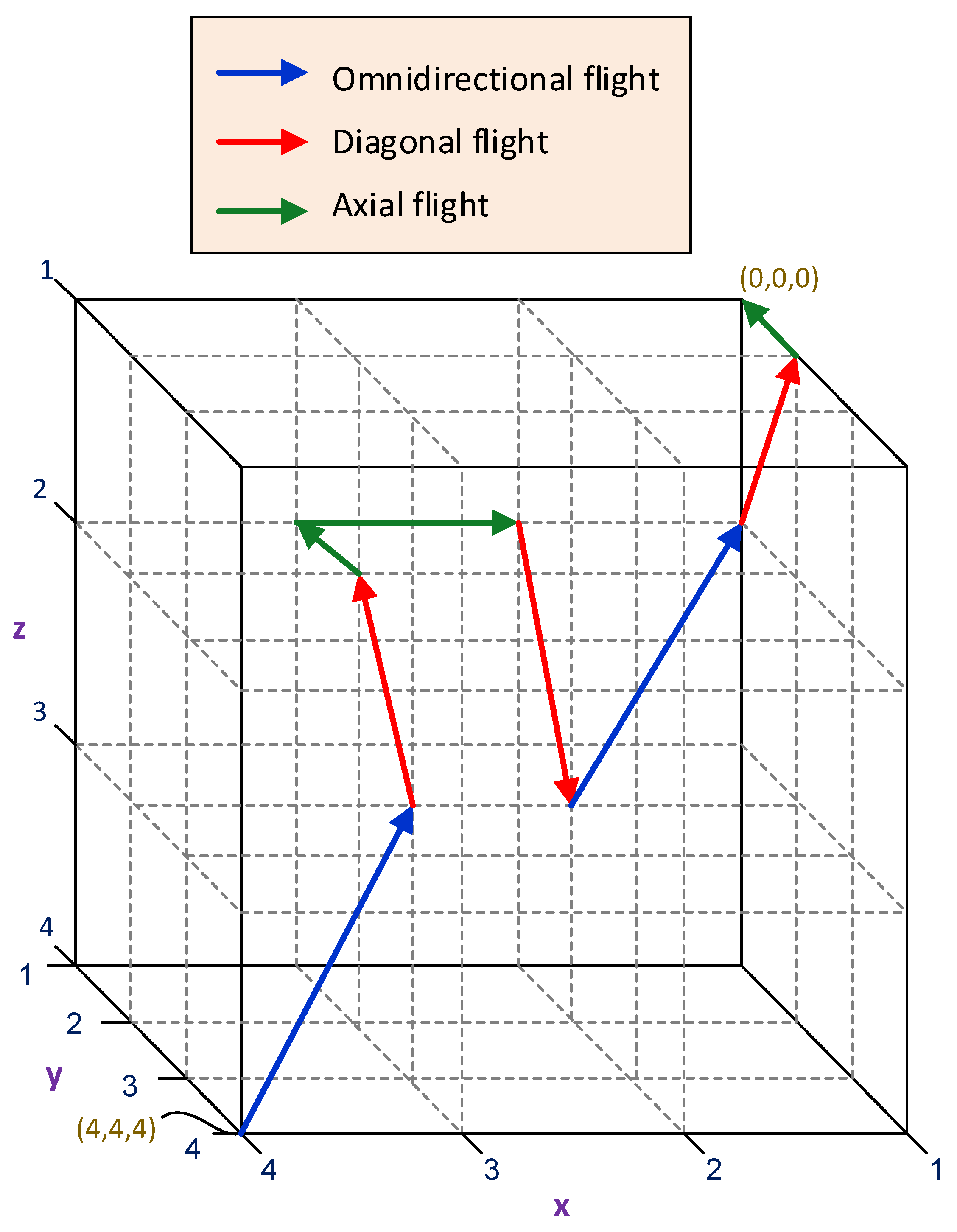
3.1. Artificial Hummingbird Algorithm (AHA)
- (a)
- Guided foraging
- (b)
- Territorial foraging
- (c)
- Migration foraging
3.2. Adaptive Opposition Artificial Hummingbird Algorithm (AOAHA)
- (a)
- Opposition-based learning
- (b)
- Adaptive decision strategy
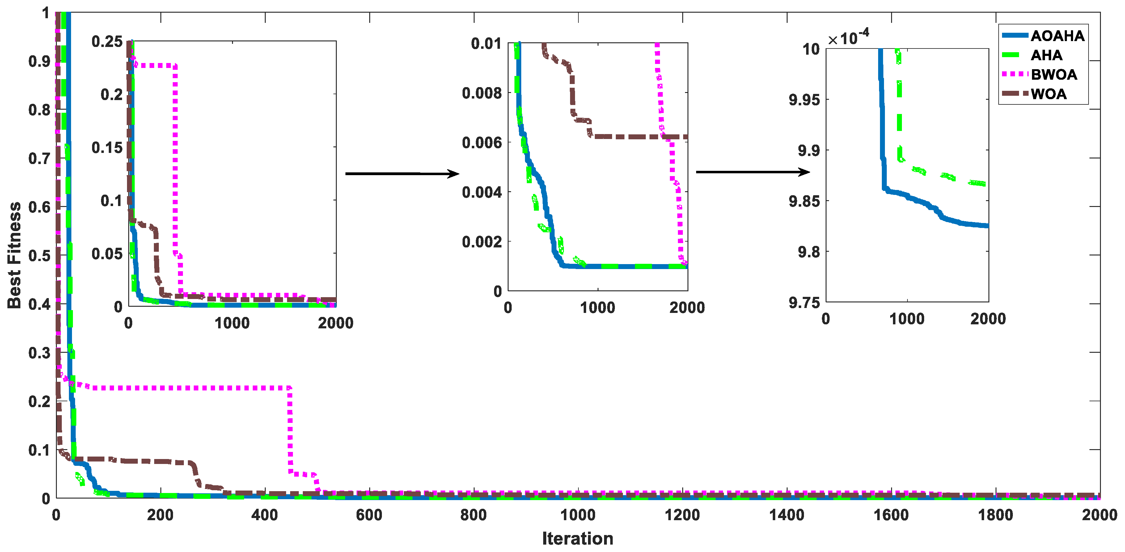
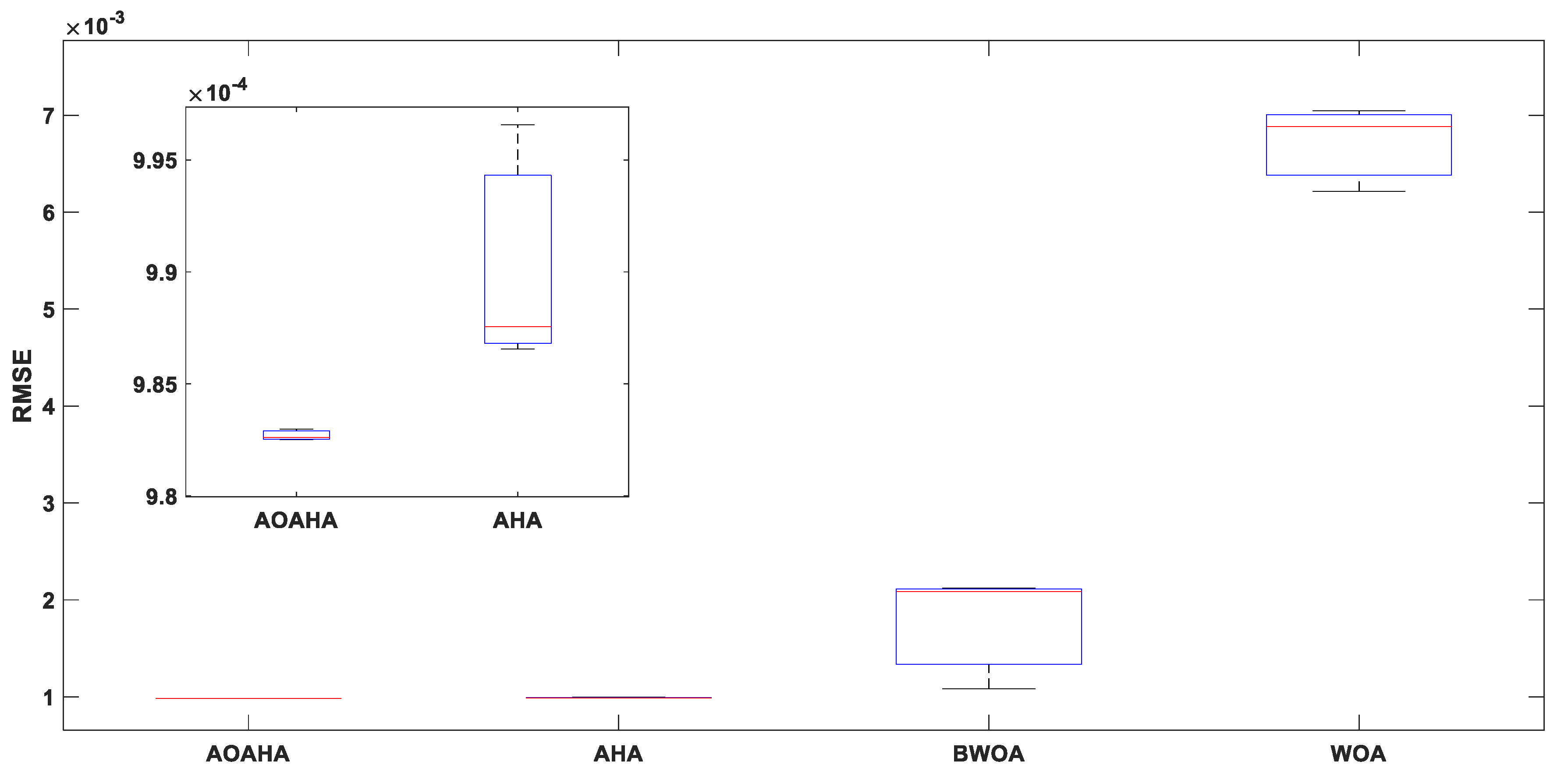
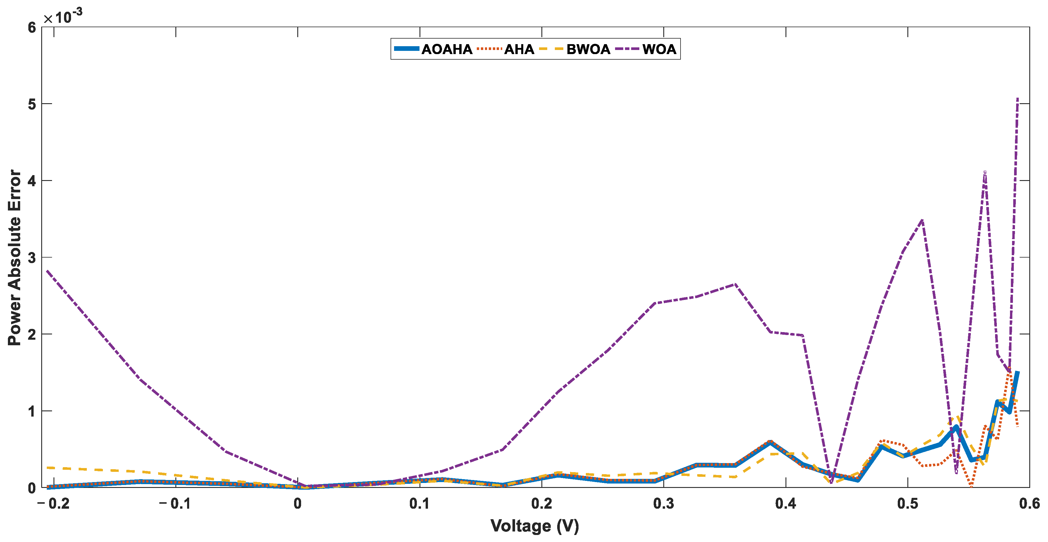
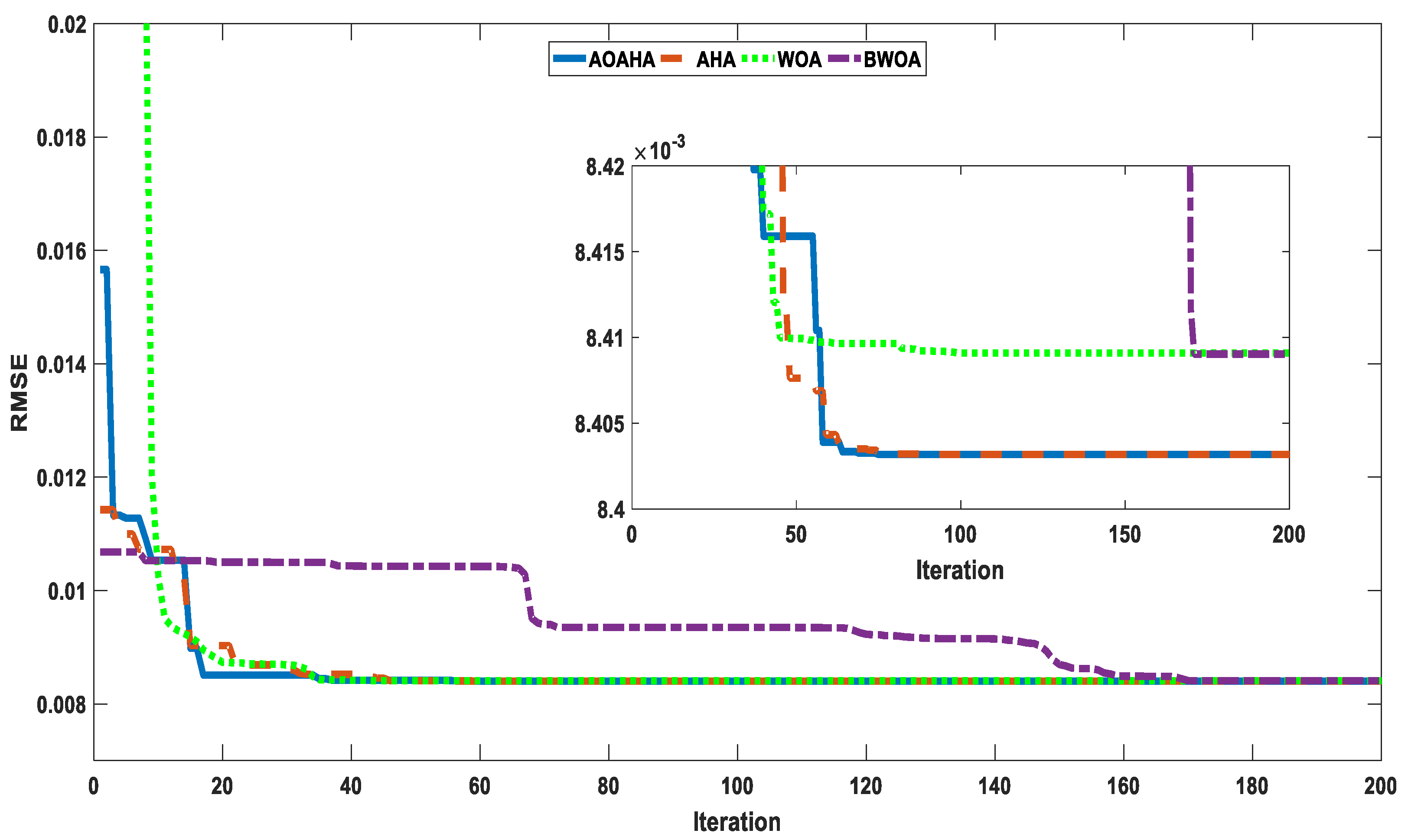
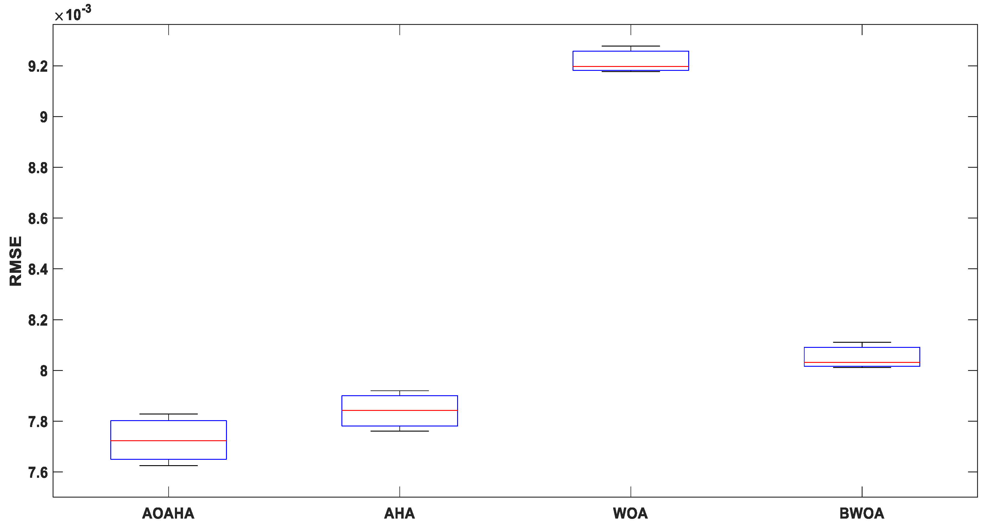
4. Results
4.1. The Performance of the AOAHA
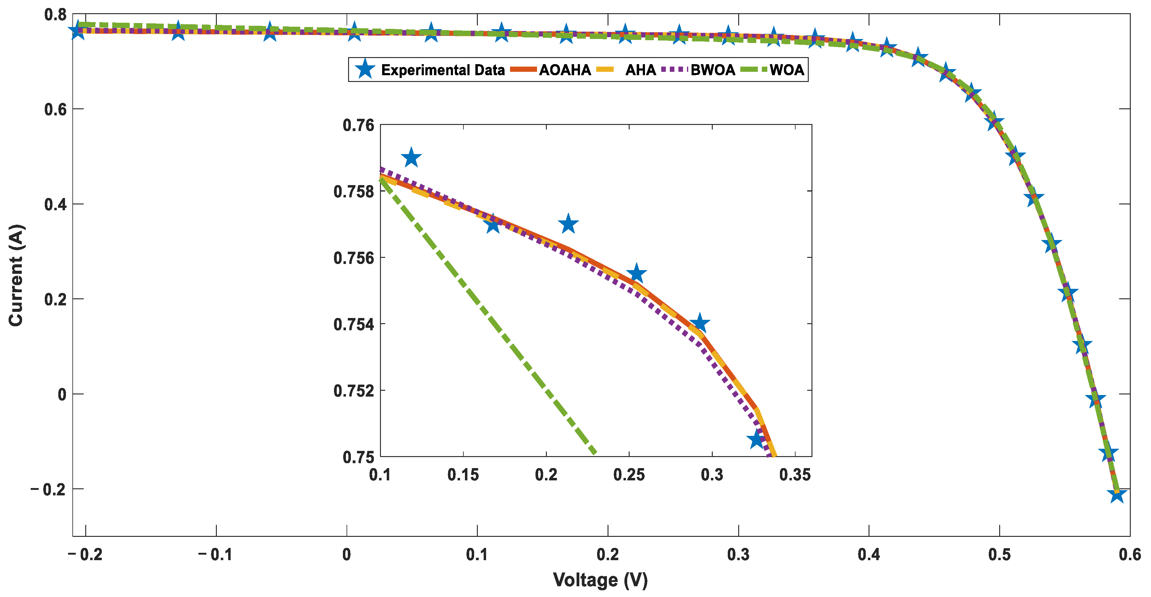
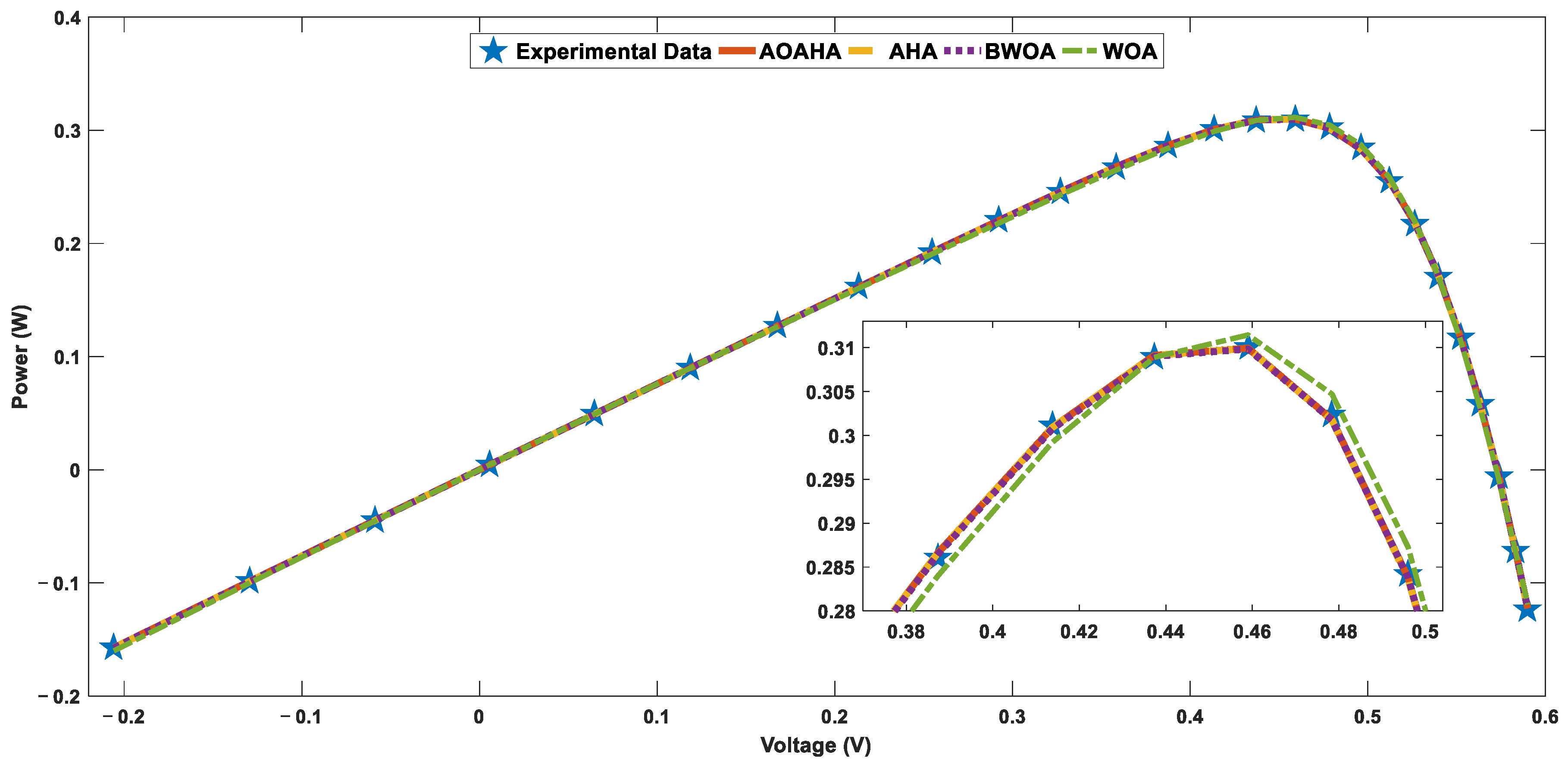
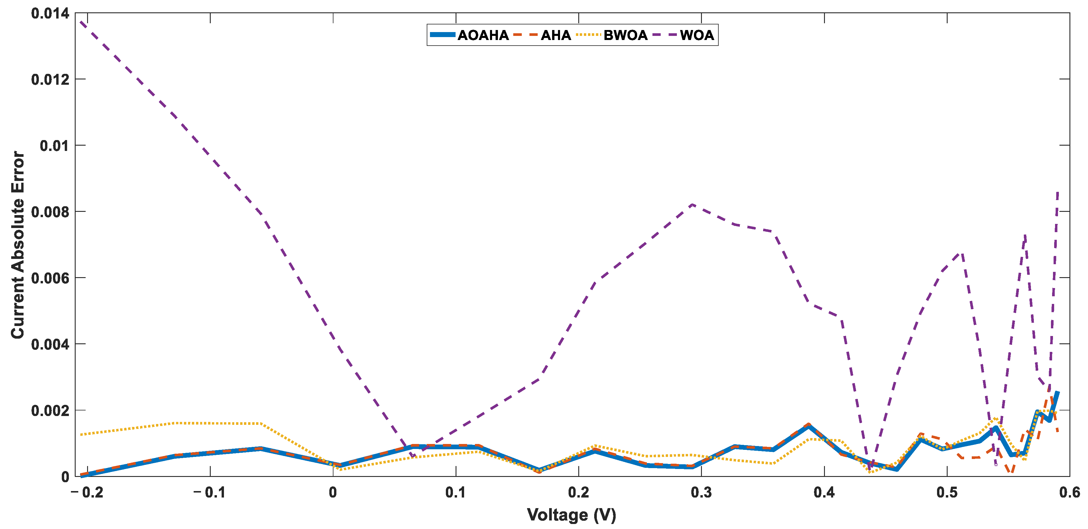
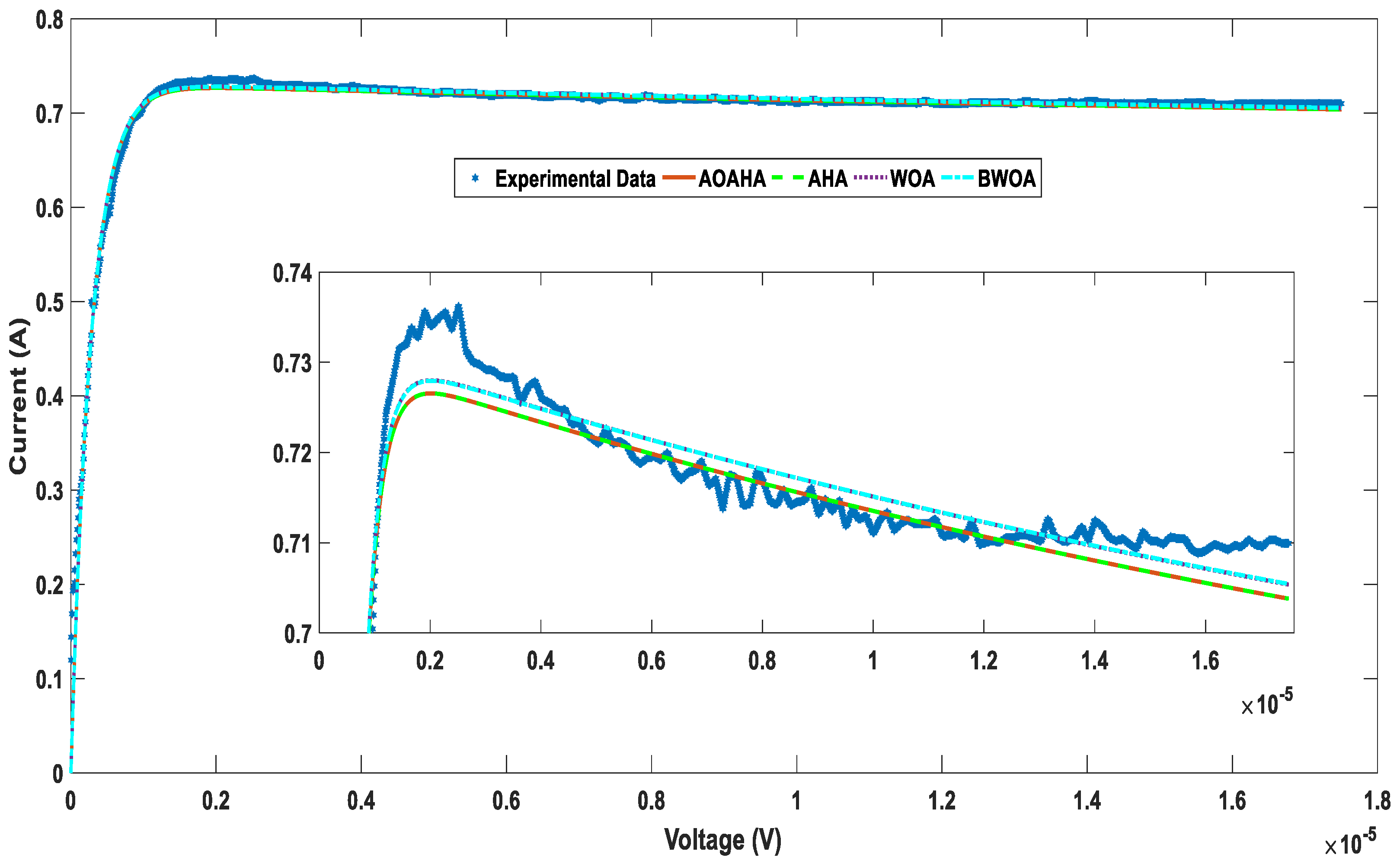
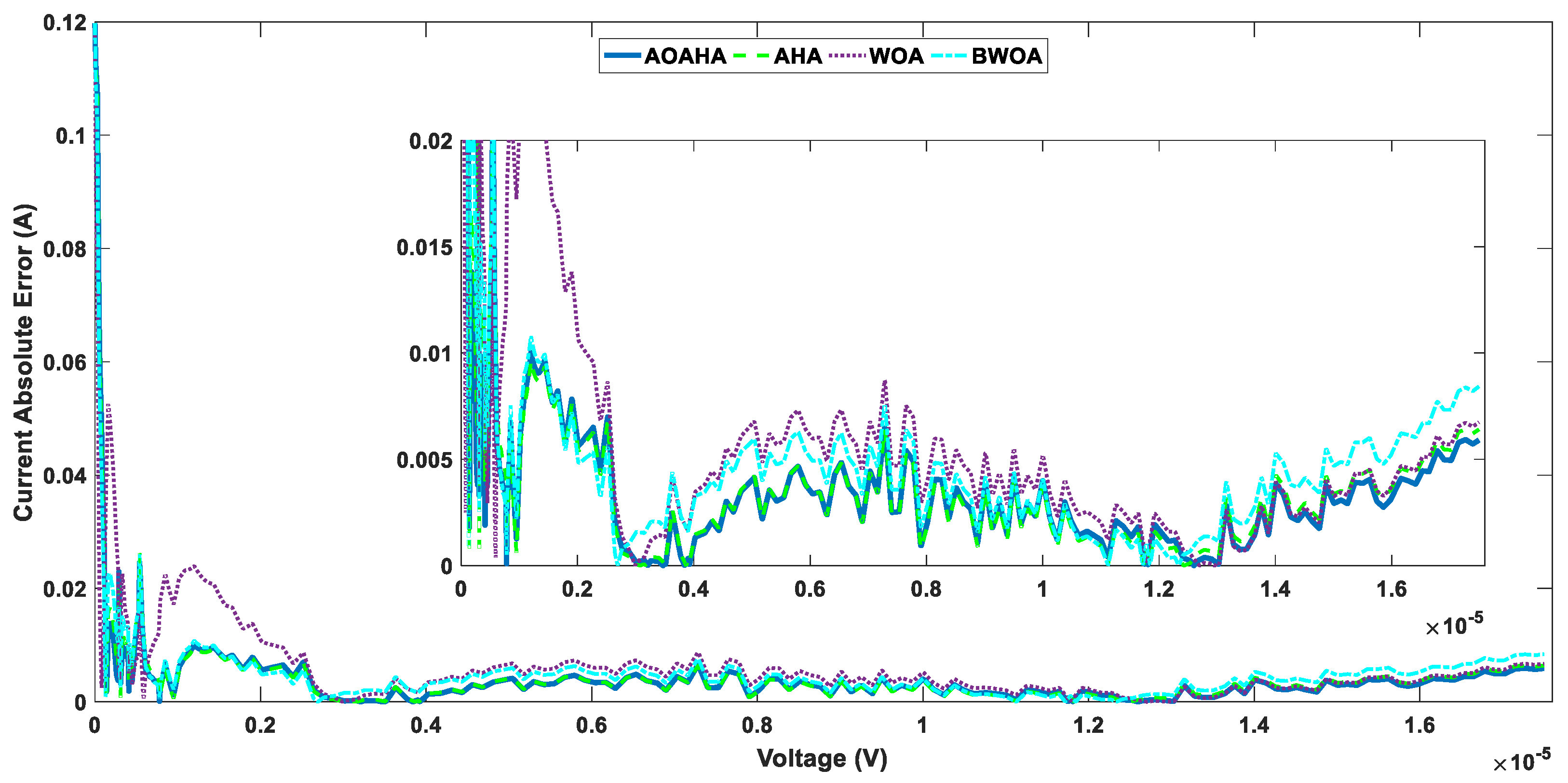
4.2. Real-World Application
4.2.1. Application 1
4.2.2. Application 2
4.2.3. Application 3
5. Conclusions
Author Contributions
Funding
Institutional Review Board Statement
Informed Consent Statement
Data Availability Statement
Conflicts of Interest
Nomenclature
| Symbol | Description |
| TDM | Three-diode model |
| DDM | Double-diode model |
| SDM | Single-diode model |
| IOM | Integral order model |
| FOM | Fractional order model |
| AHA | Artificial hummingbird algorithm |
| AOAHA | Adaptive opposition artificial hummingbird algorithm |
| PV | Photovoltaic |
| V | Terminal voltage |
| I | PV module output current |
| Iph | Current source generated from the photons |
| RMSE | Root-mean-square error |
| η1 | Ideality factor for the first diode (diffusion of current components) |
| η2 | Ideality factor for the second diode (recombination of current components) |
| T (Ko) | Photocell temperature (Kelvin) |
| η3 | Ideality factor for the third diode (leakage of current components) |
| Rs | Series resistance to represent the total resistance of the semiconductor material at neutral regions |
| Rsh | Shunt resistance to represent the total resistance for the current leakage in the P–N junction of the solar cell |
| Is1 | Current passing through the first diode |
| Is2 | Current passing through the second diode |
| K | constant of = 1.380 × 10⁻²³ (J/Ko) |
| q | 1.602 × 10⁻¹⁹ (C) coulombs. |
| ABC | Artificial bee colony |
| MPSO | Mutant particle swarm optimization |
| SSA | Salp swarm algorithm |
| ITLBO | Improved teaching–learning-based optimization |
References
- Kaliraj, P.; Devi, T. Artificial Intelligence Theory, Models, and Applications, 2nd ed.; 206 B/W Illustrations; Auerbach Publications: Boca Raton, FL, USA, 2021; p. 506. [Google Scholar]
- He, Q.; Zheng, H.; Ma, X.; Wang, L.; Kong, H.; Zhu, Z. Artificial intelligence application in a renewable energy-driven desalination system: A critical review. Energy AI 2022, 7, 100123. [Google Scholar] [CrossRef]
- Sarita, K.; Devarapalli, R.; Rai, P. Modeling and control of dynamic battery storage system used in hybrid grid. Energy Storage 2020, 2, e146. [Google Scholar] [CrossRef] [Green Version]
- Surendra, H.H.; Seshachalam, D.; Sudhindra, K.R. Design of Standalone Solar Power Plantusing System Advisor Model in Indian Context. Int. J. Recent Technol. Eng. (IJRTE) 2020, 5, 2277–3878. [Google Scholar]
- Baschieri, D.; Magni, C.A.; Marchioni, A. Comprehensive Financial Modeling of Solar PV Systems. In Proceedings of the 37th European Photovoltaic Solar Energy Conference and Exhibition, Lisbon, Portugal, 7–11 September 2020. [Google Scholar]
- Qais, M.H.; Hasanien, H.M.; Alghuwainem, S. Transient search optimization for electrical parameters estimation of photovoltaic module based on datasheet values. Energy Convers. Manag. 2020, 214, 112904. [Google Scholar] [CrossRef]
- Ramadan, A.; Kamel, S.; Korashy, A.; Yu, J. Photovoltaic Cells Parameter Estimation Using an Enhanced Teaching Learning Based Optimization Algorithm. Iran. J. Sci. Technol. 2019, 44, 767–779. [Google Scholar] [CrossRef]
- Piliougine, M.; Guejia-Burbano, R.A.; Petrone, G.; Sánchez-Pacheco, F.J.; Mora-López, L.; Sidrach-de-Cardon, M. Parameters extraction of single diode model for degraded photovoltaic modules. Renew. Energy 2021, 164, 674–686. [Google Scholar] [CrossRef]
- Ramadan, A.; Kamel, S.; Ibrahim, A.A. Parameters Estimation of Photovoltaic Cells Using Self-adaptive Multi-population Rao Optimization Algorithm. Aswan Univ. J. Sci. Technol. 2021, 31, 34. [Google Scholar]
- Stornelli, V.; Muttillo, M.; de Rubeis, T.; Nardi, I. A New Simplified Five-Parameter Estimation Method for Single-Diode Model of Photovoltaic Panels. Energies 2019, 12, 4271. [Google Scholar] [CrossRef] [Green Version]
- Messaoud, R.B. Extraction of uncertain parameters of double-diode model of a photovoltaic panel using Ant Lion Optimization. Appl. Sci. 2018, 2, 239. [Google Scholar] [CrossRef] [Green Version]
- Ramadan, A.; Kamel, S.; Taha, I.B.M.; Tostado-Véliz, M. Parameter Estimation of Modified Double-Diode and Triple-Diode Photovoltaic Models Based on Wild Horse Optimizer. Electronics 2021, 10, 2308. [Google Scholar] [CrossRef]
- Suganya, T.; Rajendran, V.; Mangaiyarkarasi, P. “Parameters Extraction of the Double Diode Model for the Polycrystalline Silicon Solar Cells” Advances in Computing and Data Sciences. ICACDS 2021. Communications in Computer and Information Science; Springer: Berlin/Heidelberg, Germany, 2021; Volume 1440. [Google Scholar]
- Yaqoob, S.J.; Saleh, A.L.; Motahhir, S.; Agyekum, E.B.; Nayyar, A.; Qureshi, B. Comparative study with practical validation of photovoltaic monocrystalline module for single and double diode models. Sci. Rep. 2021, 11, 19153. [Google Scholar] [CrossRef]
- Ramadan, A.; Kamel, S.; Hussein, M.M.; Hassan, M.H. A New Application of Chaos Game Optimization Algorithm for Parameters Extraction of Three Diode Photovoltaic model. IEEE Access 2021, 9, 51582–51594. [Google Scholar] [CrossRef]
- Houssein, E.H.; Zaki, G.N.; Diabb, A.A.Z.; Younis, E.M. An efficient Manta Ray Foraging Optimization algorithm for parameter extraction of three-diode photovoltaic model. Comput. Electr. Eng. 2021, 94, 107304. [Google Scholar] [CrossRef]
- Ramadan, A.; Kamel, S.; Khurshaid, T.; Oh, S.R.; Rhee, S.B. Parameter Extraction of Three Diode Solar Photovoltaic Model Using Improved Grey Wolf Optimizer. Sustainability 2021, 13, 6963. [Google Scholar] [CrossRef]
- Qin, L.; Xie, S.; Yang, C.; Cao, J. “Dynamic model and dynamic characteristics of solar cell” Conference Paper in Zhongguo Dianji Gongcheng Xuebao. In Proceedings of the Chinese Society of Electrical Engineering, Melbourne, Australia, 3–6 June 2013. [Google Scholar]
- Yousri, D.; Allam, D.; Eteibaa, M.B.; Suganthanb, P.N. Static and dynamic photovoltaic models’ parameters identification using Chaotic Heterogeneous Comprehensive Learning Particle Swarm Optimizer variants. Energy Convers. Manag. 2019, 182, 546–563. [Google Scholar] [CrossRef]
- Maniraj, B.; Fathima, A.P. Parameter extraction of solar photovoltaic modules using various optimization techniques: A review. J. Phys. Conf. Ser. 2020, 1716, 012001. [Google Scholar] [CrossRef]
- Venkateswari, R.; Rajasekar, N. Review on parameter estimation techniques of solar photovoltaic systems. Int. Trans. Electr. Energ. Syst. 2021, 31, e13113. [Google Scholar] [CrossRef]
- Soliman, M.A.; Al-Durra, A.; Hasanien, H.M. Electrical Parameters Identifica-tion of Three-Diode Photovoltaic Model Based on Equilibrium Optimizer Algorithm. IEEE Access 2021, 9, 41891–41901. [Google Scholar] [CrossRef]
- Joshi, H.; Arora, S. Enhanced Grey Wolf Optimization Algorithm for Global Optimization. Fundam. Inform. 2017, 153, 235–264. [Google Scholar] [CrossRef]
- Tao, Q.; Guo, H.; Li, J.; Gao, K.; Han, Y. Improved migrating birds optimization algorithm to solve hybrid flowshop scheduling problem with lot-streaming. Inst. Electr. Electron. Eng. Access 2020, 8, 89782–89792. [Google Scholar]
- Cheng, J.; Zhao, W. Chaotic enhanced colliding bodies optimization algorithm for structural reliability analysis. Adv. Struct. Eng. 2020, 23, 438–453. [Google Scholar] [CrossRef]
- Alghamdi, M.A.; Khan, M.F.N.; Khan, A.K.; Khan, I.; Ahmed, A.; Kiani, A.T.; Khan, M.A. PV Model Parameter Estimation Using Modified FPA With Dynamic Switch Probability and Step Size Function. IEEE Access 2021, 9, 42027–42044. [Google Scholar]
- Zhaoa, W.; Wanga, L.; Seyedali, M. Artificial hummingbird algorithm: A new bio-inspired optimizer with its engineering applications. Comput. Methods Appl. Mech. Eng. 2022, 388, 114194. [Google Scholar] [CrossRef]
- Naik, M.K.; Panda, R.; Abraham, A. Adaptive opposition slime mould algorithm. Soft Comput. 2021, 25, 14297–14313. [Google Scholar] [CrossRef]
- Zhao, W.; Wang, L.; Zhang, Z. Supply-demand-based optimization: A novel economics-inspired algorithm for global optimization. IEEE Access 2019, 7, 73182–73206. [Google Scholar] [CrossRef]
- Naruei, I.; Keynia, F. Wild horse optimizer: A new meta-heuristic algorithm for solving engineering optimization problems. Eng. Comput. 2021, 1–32. [Google Scholar] [CrossRef]
- Kaur, S.; Awasthi, L.K.; Sangal, A.L.; Dhiman, G. Tunicate Swarm Algorithm: A new bio-inspired based metaheuristic paradigm for global optimization. Eng. Appl. Artif. Intell. 2020, 90, 103541. [Google Scholar] [CrossRef]
- Allam, D.; Yousri, D.A.; Eteiba, M.B. Parameters extraction of the three diode model for the multi-crystalline solar cell/module using Moth-Flame Optimization Algorithm. Energy Convers. Manag. 2016, 123, 535–548. [Google Scholar] [CrossRef]
- Hafeez, G.; Javaid, N.; Iqbal, S.; Khan, F.A. Optimal Residential Load Scheduling Under Utility and Rooftop Photovoltaic Units. Energies 2018, 11, 611. [Google Scholar] [CrossRef] [Green Version]


| Function | AOAHA | AHA | SDO | WHO | TSA | |
|---|---|---|---|---|---|---|
| F1 | Best | 1.29 × 10−66 | 3.01 × 10−66 | 1.39 × 10−55 | 5.08 × 10⁻²¹ | 3.79 × 10⁻⁸ |
| Mean | 9.14 × 10−56 | 3.87 × 10−53 | 1.49 × 10−51 | 2.13 × 10⁻¹⁸ | 4.64 × 10⁻⁷ | |
| Median | 4.31 × 10−59 | 3.32 × 10−59 | 3.74 × 10−54 | 6.47 × 10⁻¹⁹ | 1.17 × 10⁻⁷ | |
| Worst | 1.54 × 10−54 | 7.66 × 10−52 | 8.43 × 10−51 | 8.56 × 10⁻¹⁸ | 4.09 × 10⁻⁶ | |
| STD | 3.48 × 10−55 | 1.71 × 10−52 | 2.99 × 10−51 | 2.98 × 10⁻¹⁸ | 1.15 × 10⁻⁶ | |
| F2 | Best | 6.71 × 10⁻³⁵ | 4.74 × 10⁻³⁴ | 1.83 × 10⁻²⁹ | 4.13 × 10⁻¹³ | 2.44 × 10⁻⁶ |
| Mean | 5.66 × 10⁻²⁹ | 1.07 × 10⁻²⁹ | 3.76 × 10⁻²⁵ | 1.3 × 10⁻¹⁰ | 1.9 × 10⁻⁵ | |
| Median | 1.12 × 10⁻³⁰ | 3.11 × 10⁻³¹ | 1.13 × 10⁻²⁶ | 5.29 × 10⁻¹¹ | 1.86 × 10⁻⁵ | |
| Worst | 4.08 × 10⁻²⁸ | 9.48 × 10⁻²⁹ | 3.98 × 10⁻²⁴ | 6.34 × 10⁻¹⁰ | 3.68 × 10⁻⁵ | |
| STD | 1.25 × 10⁻²⁸ | 2.51 × 10⁻²⁹ | 9.1 × 10⁻²⁵ | 1.77 × 10⁻¹⁰ | 9.44 × 10⁻⁶ | |
| F3 | Best | 2.43 × 10−61 | 3.15 × 10−61 | 6.27 × 10−46 | 5.13 × 10⁻¹³ | 0.027608 |
| Mean | 1.59 × 10−50 | 4.36 × 10−48 | 6.91 × 10⁻³⁴ | 1.2 × 10⁻⁸ | 1.122677 | |
| Median | 3.03 × 10−54 | 1.01 × 10−54 | 1.4 × 10−39 | 6.29 × 10⁻¹¹ | 0.772195 | |
| Worst | 3.06 × 10−49 | 6.68 × 10−47 | 1.38 × 10⁻³² | 2.3 × 10⁻⁷ | 3.914695 | |
| STD | 6.82 × 10−50 | 1.53 × 10−47 | 3.09 × 10⁻³³ | 5.14 × 10⁻⁸ | 1.096313 | |
| F4 | Best | 1.28 × 10⁻³² | 5.07 × 10⁻²⁹ | 1.11 × 10⁻²⁶ | 5.11 × 10⁻⁹ | 0.67531 |
| Mean | 3.07 × 10⁻²⁴ | 4.63 × 10⁻²⁶ | 4.52 × 10⁻²³ | 3.5 × 10⁻⁷ | 3.616654 | |
| Median | 5.11 × 10⁻²⁷ | 1.05 × 10⁻²⁷ | 1.14 × 10⁻²³ | 1 × 10⁻⁷ | 3.022253 | |
| Worst | 4.85 × 10⁻²³ | 4.23 × 10⁻²⁵ | 1.94 × 10⁻²² | 2.14 × 10⁻⁶ | 9.361516 | |
| STD | 1.11 × 10⁻²³ | 1.02 × 10⁻²⁵ | 6.34 × 10⁻²³ | 6.09 × 10⁻⁷ | 2.343658 | |
| F5 | Best | 26.8806 | 26.40974 | 27.90967 | 26.68451 | 27.18973 |
| Mean | 27.71771 | 27.5024 | 28.65096 | 37.10656 | 39.01094 | |
| Median | 27.60593 | 27.47815 | 28.74726 | 27.67985 | 28.66203 | |
| Worst | 28.73785 | 28.53304 | 28.98699 | 208.5133 | 239.7785 | |
| STD | 0.597793 | 0.472237 | 0.295026 | 40.37046 | 47.26339 | |
| F6 | Best | 0.037049 | 0.058638 | 0.039957 | 0.013248 | 2.886997 |
| Mean | 0.449979 | 0.442296 | 2.568541 | 0.064784 | 3.800719 | |
| Median | 0.36532 | 0.393054 | 2.038779 | 0.058665 | 3.736935 | |
| Worst | 1.188272 | 1.029767 | 7.250251 | 0.16971 | 4.850371 | |
| STD | 0.306108 | 0.249876 | 1.852701 | 0.043941 | 0.527851 | |
| F7 | Best | 5.14 × 10⁻⁵ | 1.47 × 10⁻⁵ | 8.66 × 10⁻⁵ | 0.000605 | 0.007604 |
| Mean | 0.000397 | 0.000346 | 0.002356 | 0.001779 | 0.019206 | |
| Median | 0.000335 | 0.000219 | 0.001136 | 0.001387 | 0.018479 | |
| Worst | 0.001143 | 0.001202 | 0.013813 | 0.004938 | 0.04436 | |
| STD | 0.000298 | 0.000292 | 0.003331 | 0.001255 | 0.007628 | |
| Function | AOAHA | AHA | SDO | WHO | TSA | |
|---|---|---|---|---|---|---|
| F8 | Best | −1678.77 | −1724.06 | −1655 | −1807.46 | −1394.45 |
| Mean | −1551.15 | −1551.13 | −1312.83 | −1721.44 | −1212.82 | |
| Median | −1544.23 | −1562.44 | −1385.86 | −1729.69 | −1232.52 | |
| Worst | −1443.17 | −1364.15 | −598.802 | −1630.81 | −976.635 | |
| STD | 69.17895 | 93.45685 | 294.008 | 54.13894 | 122.0762 | |
| F9 | Best | 0.00 | 0.00 | 4.33 × 10⁻³⁰ | 0.00 | 156.667 |
| Mean | 0.00 | 0.00 | 1.75 × 10⁻²² | 1.11 × 10⁻⁵ | 228.0177 | |
| Median | 0.00 | 0.00 | 4.17 × 10⁻²⁵ | 1 × 10⁻⁹ | 228.634 | |
| Worst | 0.00 | 0.00 | 3.02 × 10⁻²¹ | 0.000177 | 331.7581 | |
| STD | 0.00 | 0.00 | 6.75 × 10⁻²² | 3.96 × 10⁻⁵ | 46.40919 | |
| F10 | Best | 8.88 × 10⁻¹⁶ | 8.88 × 10⁻¹⁶ | 8.88 × 10⁻¹⁶ | 8.88 × 10⁻¹⁶ | 20.81133 |
| Mean | 8.88 × 10⁻¹⁶ | 8.88 × 10⁻¹⁶ | 8.88 × 10⁻¹⁶ | 1.003597 | 20.9608 | |
| Median | 8.88 × 10⁻¹⁶ | 8.88 × 10⁻¹⁶ | 8.88 × 10⁻¹⁶ | 7.99 × 10⁻⁶ | 20.99356 | |
| Worst | 8.88 × 10⁻¹⁶ | 8.88 × 10⁻¹⁶ | 8.88 × 10⁻¹⁶ | 20.01369 | 21.0961 | |
| STD | 0.00 | 0.00 | 0.00 | 4.474524 | 0.091505 | |
| F11 | Best | 0.00 | 0.00 | 0.00 | 0.00 | 1.3 × 10⁻⁹ |
| Mean | 0.00 | 0.00 | 0.00 | 1.83 × 10⁻¹⁶ | 0.007018 | |
| Median | 0.00 | 0.00 | 0.00 | 0.00 | 1.44 × 10⁻⁸ | |
| Worst | 0.00 | 0.00 | 0.00 | 3.66 × 10⁻¹⁵ | 0.029126 | |
| STD | 0.00 | 0.00 | 0.00 | 8.19 × 10⁻¹⁶ | 0.010243 | |
| F12 | Best | 0.00112 | 0.001029 | 0.001152 | 4.64 × 10⁻⁵ | 0.374956 |
| Mean | 0.009553 | 0.008654 | 0.23467 | 0.026544 | 2.805889 | |
| Median | 0.009173 | 0.006918 | 0.067805 | 0.000309 | 2.009833 | |
| Worst | 0.020446 | 0.031416 | 1.492821 | 0.207386 | 7.656863 | |
| STD | 0.005674 | 0.007552 | 0.352063 | 0.056802 | 2.128936 | |
| F13 | Best | 0.433176 | 1.456302 | 0.046216 | 0.011802 | 2.372295 |
| Mean | 2.155627 | 2.339115 | 1.867552 | 0.173897 | 3.298085 | |
| Median | 2.401709 | 2.436057 | 1.934246 | 0.136817 | 3.22876 | |
| Worst | 2.969199 | 2.969591 | 2.999924 | 0.700833 | 4.16073 | |
| STD | 0.723935 | 0.361111 | 0.961284 | 0.157716 | 0.565835 | |
| Function | AOAHA | AHA | SDO | WHO | TSA | |
|---|---|---|---|---|---|---|
| F14 | Best | 0.998004 | 0.998004 | 0.998004 | 0.998004 | 0.998004 |
| Mean | 0.998004 | 0.998004 | 3.494696 | 1.097209 | 8.298683 | |
| Median | 0.998004 | 0.998004 | 1.495017 | 0.998004 | 10.76318 | |
| Worst | 0.998004 | 0.998004 | 12.67051 | 2.982105 | 18.30431 | |
| STD | 1.76 × 10⁻⁸ | 1.03 × 10⁻⁹ | 3.953203 | 0.443659 | 5.533952 | |
| F15 | Best | 0.000307 | 0.000307 | 0.000307 | 0.000307 | 0.000308 |
| Mean | 0.000308 | 0.000318 | 0.00067 | 0.000602 | 0.007136 | |
| Median | 0.000308 | 0.000308 | 0.000527 | 0.000593 | 0.000505 | |
| Worst | 0.00032 | 0.000485 | 0.002121 | 0.001223 | 0.031699 | |
| STD | 2.69 × 10⁻⁶ | 3.95 × 10⁻⁵ | 0.000473 | 0.000286 | 0.010606 | |
| F16 | Best | −1.03163 | −1.03163 | −1.03163 | −1.03163 | −1.03163 |
| Mean | −1.03163 | −1.03163 | −1.03005 | −1.03163 | −1.0253 | |
| Median | −1.03163 | −1.03163 | −1.03163 | −1.03163 | −1.03163 | |
| Worst | −1.03163 | −1.03163 | −1.00046 | −1.03163 | −0.99999 | |
| STD | 1.3 × 10⁻¹² | 1.18 × 10⁻¹² | 0.006966 | 5.09 × 10⁻¹⁷ | 0.012981 | |
| F17 | Best | 0.397887 | 0.397887 | 0.397887 | 0.397887 | 0.39789 |
| Mean | 0.397887 | 0.397887 | 0.397987 | 0.397887 | 0.397927 | |
| Median | 0.397887 | 0.397887 | 0.397887 | 0.397887 | 0.397907 | |
| Worst | 0.397887 | 0.397887 | 0.399795 | 0.397887 | 0.398082 | |
| STD | 0.00 | 0.00 | 0.000426 | 0.00 | 4.53 × 10⁻⁵ | |
| F18 | Best | 3.00 | 3.00 | 3.00 | 3.00 | 3.000009 |
| Mean | 3.00 | 3.00 | 3.00 | 3.00 | 8.400078 | |
| Median | 3.00 | 3.00 | 3.00 | 3.00 | 3.000084 | |
| Worst | 3.00 | 3.00 | 3.00 | 3.00 | 84.00001 | |
| STD | 1.77 × 10⁻¹⁵ | 1.6 × 10⁻¹⁵ | 5.21 × 10⁻⁸ | 1.13 × 10⁻¹⁵ | 18.78799 | |
| F19 | Best | −0.30048 | −0.30048 | −0.30048 | −0.30048 | −0.30048 |
| Mean | −0.30047 | −0.30047 | −0.2893 | −0.30048 | −0.30048 | |
| Median | −0.30047 | −0.30047 | −0.30038 | −0.30048 | −0.30048 | |
| Worst | −0.30046 | −0.30044 | −0.19165 | −0.30048 | −0.30048 | |
| STD | 4.22 × 10⁻⁶ | 1.04 × 10⁻⁵ | 0.026531 | 1.14 × 10⁻¹⁶ | 1.14 × 10⁻¹⁶ | |
| F20 | Best | −3.322 | −3.322 | −3.322 | −3.322 | −3.32148 |
| Mean | −3.29227 | −3.30415 | −3.09697 | −3.21756 | −3.07223 | |
| Median | −3.322 | −3.322 | −3.2031 | −3.322 | −3.20118 | |
| Worst | −3.2031 | −3.2031 | −0.89904 | −2.43178 | −0.20816 | |
| STD | 0.052819 | 0.043552 | 0.550986 | 0.239908 | 0.679321 | |
| F21 | Best | −10.1532 | −10.1532 | −10.1532 | −10.1532 | −10.0895 |
| Mean | −9.89798 | −10.1059 | −8.703 | −9.77706 | −5.89545 | |
| Median | −10.1531 | −10.153 | −10.1532 | −10.1532 | −4.90994 | |
| Worst | −5.0552 | −9.2237 | −4.99677 | −2.63047 | −2.58642 | |
| STD | 1.139873 | 0.207648 | 2.23952 | 1.682133 | 2.775111 | |
| F22 | Best | −10.4029 | −10.4029 | −10.4029 | −10.4029 | −10.3637 |
| Mean | −10.135 | −10.0864 | −8.45822 | −9.75463 | −7.02119 | |
| Median | −10.4029 | −10.4029 | −10.4029 | −10.4029 | −9.8942 | |
| Worst | −5.08767 | −5.08767 | −1.0677 | −2.75193 | −1.82478 | |
| STD | 1.188023 | 1.19136 | 3.128689 | 2.031123 | 3.57071 | |
| F23 | Best | −10.5364 | −10.5364 | −10.5364 | −10.5364 | −10.4599 |
| Mean | −10.1167 | −10.2621 | −7.90449 | −10.5364 | −5.50502 | |
| Median | −10.5364 | −10.5364 | −10.5357 | −10.5364 | −2.83596 | |
| Worst | −5.12848 | −5.12848 | −3.79083 | −10.5364 | −1.66783 | |
| STD | 1.348528 | 1.208388 | 3.015319 | 1.58 × 10⁻¹⁵ | 3.728197 | |
| Parameter | Solar Cell | |
|---|---|---|
| Lower Limit | Upper Limit | |
| Rs | 0 | 5 |
| Rsh | 0 | 100 |
| Iph | 0 | 2 |
| Is1 | 0 | 1 |
| Is2 | 0 | 1 |
| Is3 | 0 | 1 |
| ɳ1 | 1 | 2 |
| ɳ2 | 1 | 2 |
| ɳ3 | 1 | 2 |
| AOAHA | AHA | BWOA | WOA | |
|---|---|---|---|---|
| Rs (Ω) | 0.03674 | 0.036509 | 0.036424 | 0.045276 |
| Rsh(Ω) | 55.41315 | 54.16416 | 46.36289 | 15.77225 |
| Iph(A) | 0.76078 | 0.760772 | 0.761422 | 0.766883 |
| Is1(A) | 7.37 × 10⁻⁷ | 4.00 × 10⁻⁸ | 1.50 × 10⁻⁷ | 1.72 × 10⁻⁸ |
| Is2(A) | 1.13 × 10⁻⁷ | 2.98 × 10⁻⁷ | 1.49 × 10⁻⁷ | 1.30 × 10⁻¹⁰ |
| Is3(A) | 1.17 × 10⁻⁷ | 2.39 × 10⁻⁸ | 1.50 × 10⁻⁷ | 6.51 × 10⁻¹⁰ |
| η1 | 1.999589 | 1.39016 | 1.504014 | 1.232062 |
| η2 | 1.46187 | 1.51173 | 1.446121 | 1.85067 |
| η3 | 1.43712 | 1.562159 | 1.982461 | 1.850237 |
| RMSE | 0.0009825181 | 0.0009865625 | 0.0010846 | 0.0062131083 |
| Minimum | Average | Maximum | STD | |
|---|---|---|---|---|
| AOAHA | 0.0009825181 | 0.000982709 | 0.000982992 | 2.49687 × 10⁻⁷ |
| AHA | 0.0009865625 | 0.000990229 | 0.000996563 | 5.50757 × 10⁻⁶ |
| BWOA | 0.0010846 | 0.0017644 | 0.002124 | 0.000589054 |
| WOA | 0.0062131083 | 0.006712806 | 0.007044 | 0.00044033 |
| Parameter | Solar Cell | |
|---|---|---|
| Lower Limit | Upper Limit | |
| Rs | 0 | 5 |
| Rsh | 0 | 5000 |
| Iph | 0 | 2 |
| Is1 | 0 | 1 |
| Is2 | 0 | 1 |
| Is3 | 0 | 1 |
| η1 | 1 | 50 |
| η2 | 1 | 50 |
| η3 | 1 | 50 |
| Irradiance Level | Parameters | ||||||||||
|---|---|---|---|---|---|---|---|---|---|---|---|
| Rs | Rsh | Iph | Is1 | Is2 | Is3 | η1 | η2 | η3 | RMSE | ||
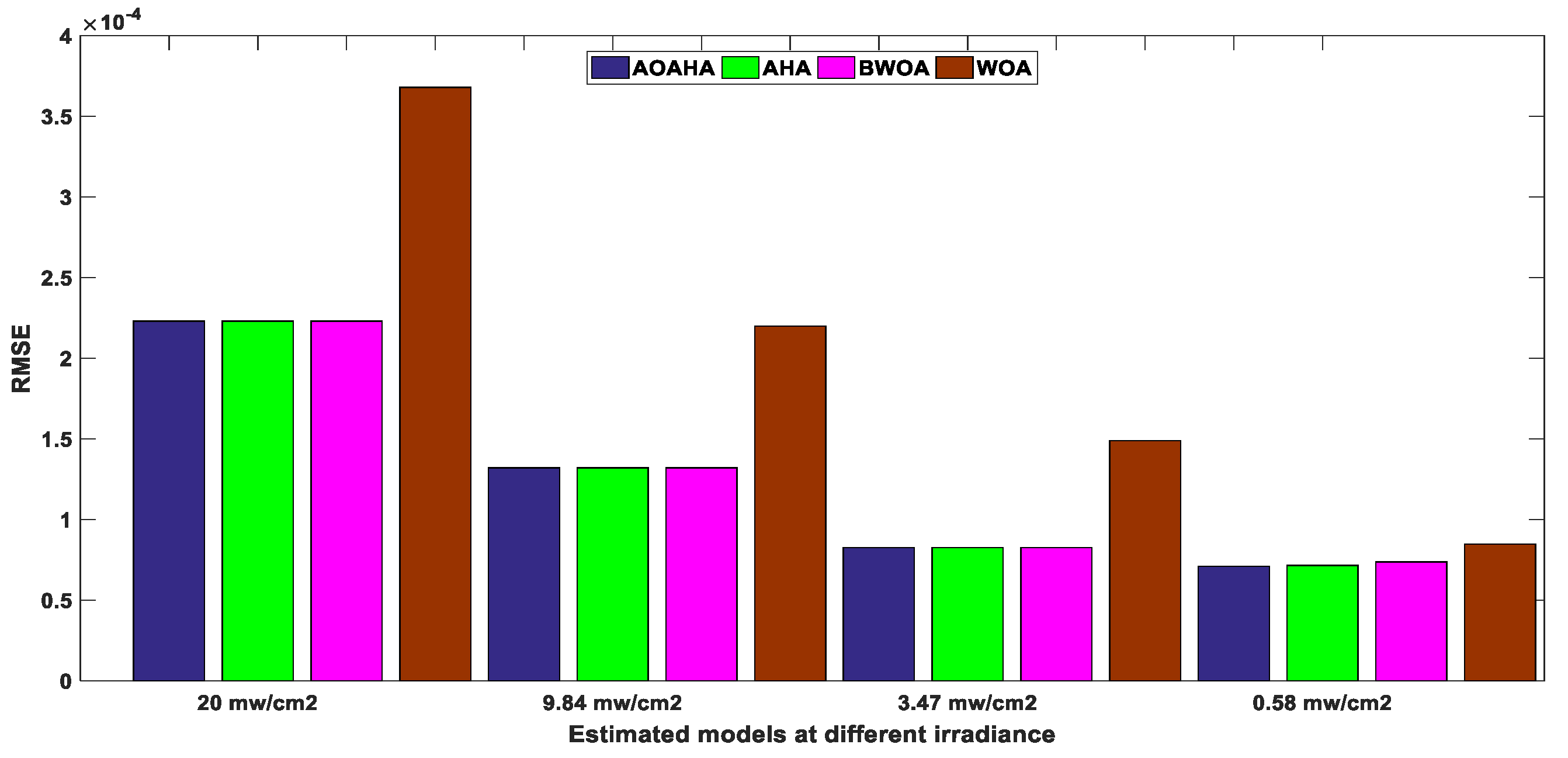
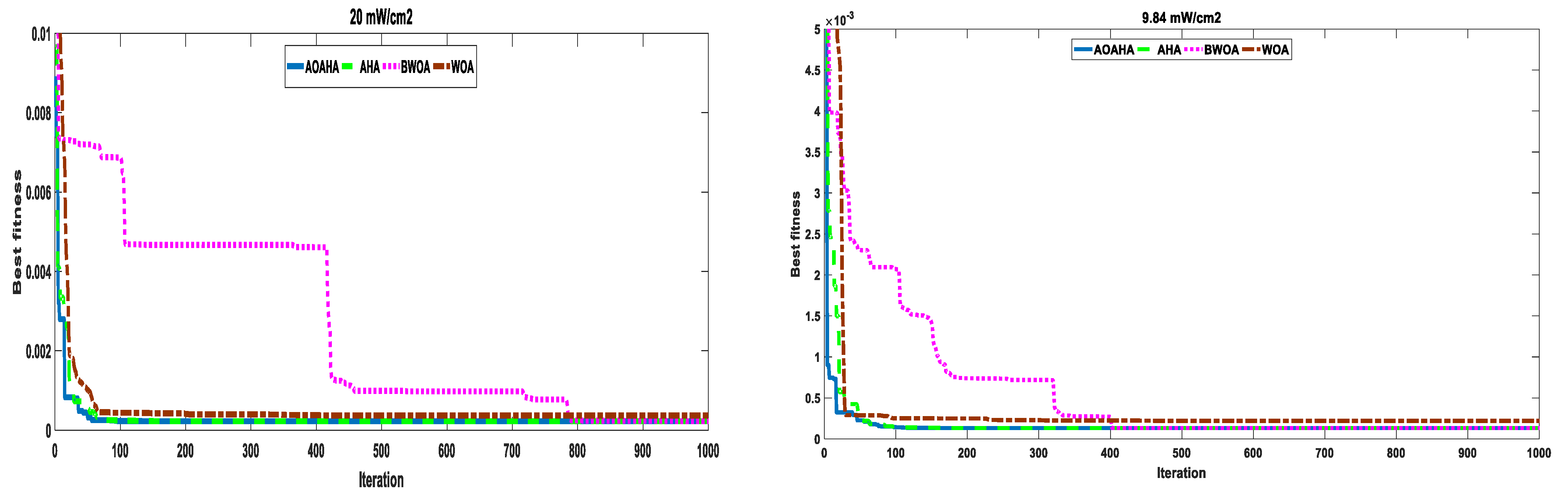
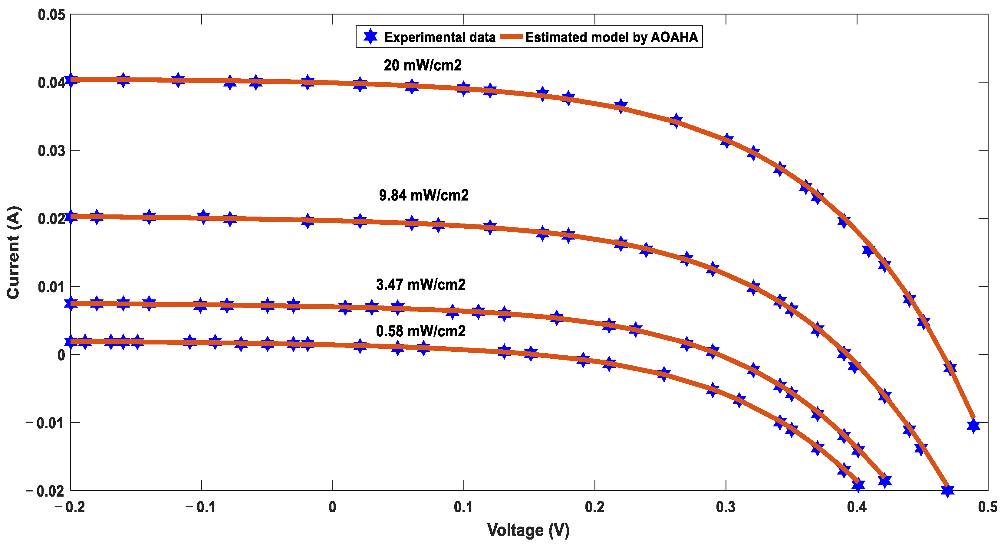
| At 20 mw/cm2 | AOAHA | 0.0895 | 5000.00 | 0.0399 | 0.0005289 | 2.08 × 10⁻¹⁰ | 2.39 × 10⁻¹⁰ | 4.1698 | 4.1698 | 4.1698 | 2.23 × 10⁻⁴ |
| AHA | 0.0895 | 5000.00 | 0.0399 | 2.33 × 10⁻¹⁰ | 0.000528 | 4.37 × 10⁻¹⁰ | 4.1699 | 4.1698 | 4.1699 | 2.23 × 10⁻⁴ | |
| BWOA | 0.0914 | 5000.00 | 0.0399 | 0.0005271 | 1.16 × 10⁻⁶ | 6.08 × 10⁻¹⁶ | 4.1664 | 27.1378 | 27.1375 | 2.23 × 10⁻⁴ | |
| WOA | 0.3963 | 208.77 | 0.0399 | 1.18 × 10⁻²⁰ | 1.07 × 10⁻²⁰ | 0.0002302 | 25.4707 | 1.0696 | 3.5395 | 3.68 × 10⁻⁴ | |
| At 9.84 mw/cm2 | AOAHA | 0.7072 | 579.49 | 0.0197 | 0.000247 | 2.95 × 10⁻⁵ | 0.0001220 | 3.4987 | 49.2649 | 46.6918 | 1.32 × 10⁻⁴ |
| AHA | 0.7057 | 545.48 | 0.0197 | 1.49 × 10⁻¹⁰ | 9.74 × 10⁻¹⁰ | 0.00024880 | 38.9430 | 45.8783 | 3.5019 | 1.32 × 10⁻⁴ | |
| BWOA | 0.7057 | 545.52 | 0.0197 | 0.0002488 | 1.00 × 10⁻²⁰ | 1.00 × 10⁻²⁰ | 3.5019 | 4.8614 | 29.4960 | 1.32 × 10⁻⁴ | |
| BWOA | 0.1759 | 591.45 | 0.0197 | 0.0004273 | 2.02 × 10⁻²⁰ | 2.02 × 10⁻²⁰ | 3.9971 | 1.9377 | 2.0179 | 2.20 × 10⁻⁴ | |
| At 3.47 mw/cm2 | AOAHA | 1.1300 | 611.16 | 0.0070 | 2.64 × 10⁻⁸ | 1.76 × 10⁻⁴ | 1.30 × 10⁻⁹ | 40.9859 | 3.1423 | 39.6484 | 8.26 × 10⁻⁵ |
| AHA | 1.1330 | 801.83 | 0.0070 | 3.57 × 10⁻⁶ | 1.73 × 10⁻⁴ | 0.00052421 | 44.3793 | 3.1341 | 47.8092 | 8.27 × 10⁻⁵ | |
| BWOA | 1.1301 | 611.05 | 0.0070 | 1.41 × 10⁻¹⁹ | 1.86 × 10⁻¹⁵ | 0.00017578 | 49.9954 | 9.5640 | 3.1422 | 8.26 × 10⁻⁵ | |
| BWOA | 0.0752 | 1224.95 | 0.0070 | 7.02 × 10⁻²⁰ | 0.000370 | 2.35 × 10⁻²⁰ | 6.0038 | 3.8487 | 45.0651 | 1.49 × 10⁻⁴ | |
| At 0.58 mw/cm2 | AOAHA | 1.4704 | 4996.03 | 0.0014 | 0.000748 | 0.000105 | 3.25 × 10⁻⁶ | 10.2939 | 2.8197 | 14.9268 | 7.15 × 10⁻⁵ |
| AHA | 1.5406 | 4944.53 | 0.0014 | 7.91 × 10⁻⁵ | 4.14 × 10⁻⁶ | 0.00065080 | 2.6899 | 21.0457 | 7.9911 | 7.10 × 10⁻⁵ | |
| BWOA | 1.2021 | 956.54 | 0.0014 | 0.0005149 | 0.000173 | 1.00 × 10⁻²⁰ | 17.6110 | 3.1138 | 49.9999 | 7.37 × 10⁻⁵ | |
| BWOA | 0.4513 | 1133.55 | 0.0014 | 0.0003144 | 1.60 × 10⁻¹⁹ | 5.35 × 10⁻¹⁹ | 3.6546 | 43.9120 | 45.4858 | 8.48 × 10⁻⁵ | |
| Parameter | Solar Cell | |
|---|---|---|
| Lower Limit | Upper Limit | |
| 0 | 20 | |
| 2 × 10⁻⁸ | 6 × 10⁻⁵ | |
| 5 × 10⁻⁶ | 1× 10⁻⁴ | |
| 0.8 | 1.1 | |
| 0.8 | 1.1 | |
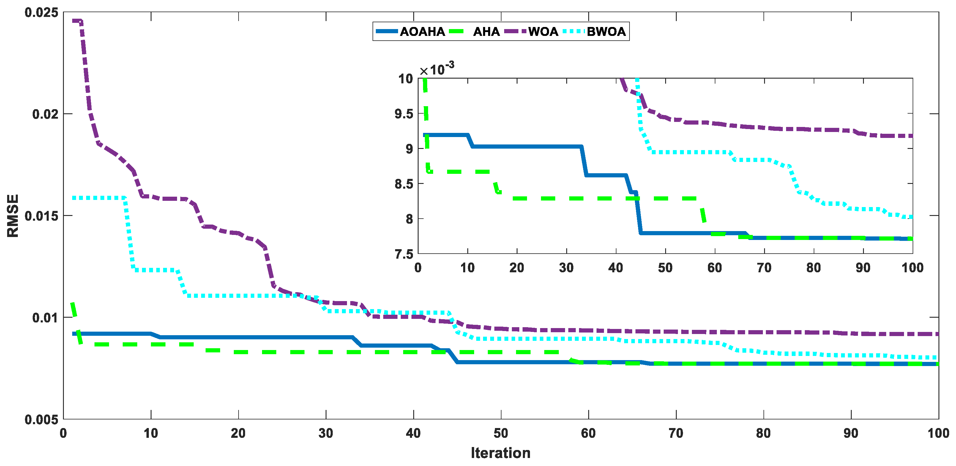
| AOAHA | AHA | WOA | BWOA | |
|---|---|---|---|---|
| 13.79387624 | 13.79388 | 13.06099 | 13.06404 | |
| 1.57 × 10⁻⁶ | 1.57 × 10⁻⁶ | 1.70 × 10⁻⁶ | 1.71 × 10⁻⁶ | |
| 7.50 × 10⁻⁶ | 7.50 × 10⁻⁶ | 7.50 × 10⁻⁶ | 7.50 × 10⁻⁶ | |
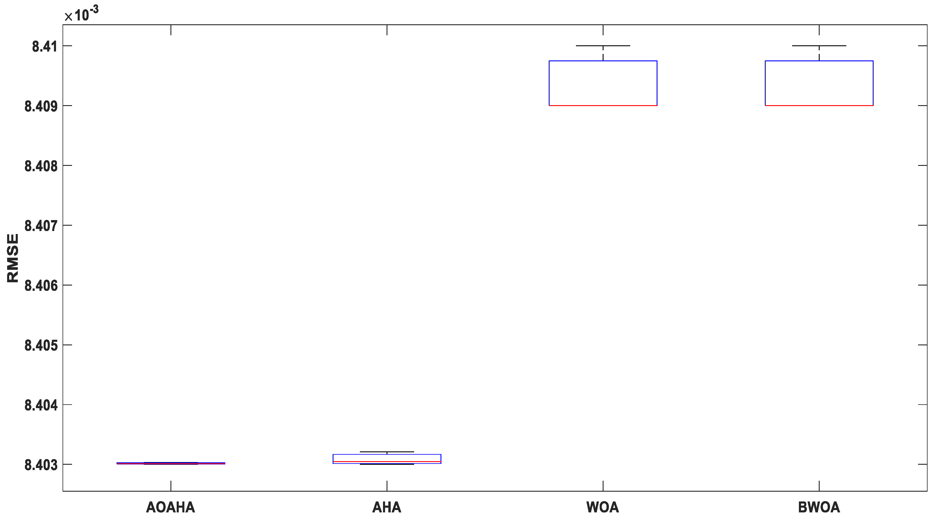
| RMSE | 0.008403 | 0.008403 | 0.008409 | 0.008409 |
| AOAHA | AHA | WOA | BWOA | |
|---|---|---|---|---|
| 6.668716 | 6.552183 | 3.513184 | 6.162661 | |
| 9.92 × 10⁻⁶ | 9.31 × 10⁻⁶ | 1.47 × 10⁻⁵ | 3.23 × 10⁻⁶ | |
| 1.65 × 10⁻⁵ | 1.69 × 10⁻⁵ | 9.48 × 10⁻⁵ | 2.12 × 10⁻⁵ | |
| 0.845127 | 0.84893 | 0.807758 | 0.93991 | |
| 0.945356 | 0.943134 | 0.823822 | 0.927025 | |
| RMSE | 0.007712 | 0.007712 | 0.009177 | 0.008011 |
| Minimum | Average | Maximum | STD | |
|---|---|---|---|---|
| AOAHA | 0.008403003 | 0.008403012 | 0.008403032 | 1.16558 × 10⁻⁸ |
| AHA | 0.008403003 | 0.008403046 | 0.008403207 | 9.03883 × 10⁻⁸ |
| WOA | 0.008409 | 0.008409 | 0.00841 | 3.94 × 10⁻⁷ |
| BWOA | 0.008409 | 0.008409 | 0.00841 | 3.36 × 10⁻⁷ |
| Minimum | Average | Maximum | STD | |
|---|---|---|---|---|
| AOAHA | 0.0076253586 | 0.0077234518 | 0.0078285384 | 9.06109 × 10⁻⁵ |
| AHA | 0.0077604697 | 0.0078421887 | 0.0079199453 | 6.59704 × 10⁻⁵ |
| WOA | 0.009177 | 0.0091974 | 0.009278 | 4.50571 × 10⁻⁵ |
| BWOA | 0.0080114 | 0.0080315 | 0.008111 | 4.44423 × 10⁻⁵ |
Publisher’s Note: MDPI stays neutral with regard to jurisdictional claims in published maps and institutional affiliations. |
© 2022 by the authors. Licensee MDPI, Basel, Switzerland. This article is an open access article distributed under the terms and conditions of the Creative Commons Attribution (CC BY) license (https://creativecommons.org/licenses/by/4.0/).
Share and Cite
Ramadan, A.; Kamel, S.; Hassan, M.H.; Ahmed, E.M.; Hasanien, H.M. Accurate Photovoltaic Models Based on an Adaptive Opposition Artificial Hummingbird Algorithm. Electronics 2022, 11, 318. https://doi.org/10.3390/electronics11030318
Ramadan A, Kamel S, Hassan MH, Ahmed EM, Hasanien HM. Accurate Photovoltaic Models Based on an Adaptive Opposition Artificial Hummingbird Algorithm. Electronics. 2022; 11(3):318. https://doi.org/10.3390/electronics11030318
Chicago/Turabian StyleRamadan, Abdelhady, Salah Kamel, Mohamed H. Hassan, Emad M. Ahmed, and Hany M. Hasanien. 2022. "Accurate Photovoltaic Models Based on an Adaptive Opposition Artificial Hummingbird Algorithm" Electronics 11, no. 3: 318. https://doi.org/10.3390/electronics11030318
APA StyleRamadan, A., Kamel, S., Hassan, M. H., Ahmed, E. M., & Hasanien, H. M. (2022). Accurate Photovoltaic Models Based on an Adaptive Opposition Artificial Hummingbird Algorithm. Electronics, 11(3), 318. https://doi.org/10.3390/electronics11030318