SARIMA: A Seasonal Autoregressive Integrated Moving Average Model for Crime Analysis in Saudi Arabia

Abstract

Crimes have clearly had a detrimental impact on a nation’s development, prosperity, reputation, and economy. The issue of crime has become one of the most pressing concerns in societies, thus reducing the crime rate has become an increasingly critical task. Recently, several studies have been proposed to identify the causes and occurrences of crime in order to identify ways to reduce crime rates. However, few studies have been conducted in Saudi Arabia technological solutions based on crime analysis. The analysis of crime can help governments identify hotspots of crime and monitor crime distribution. This study aims to investigate which Saudi Arabian areas will experience increased crime rates in the coming years. This research helps law enforcement agencies to effectively utilize available resources in order to reduce crime rates. This paper proposes SARIMA model which focuses on identifying factors that affect crimes in Saudi Arabia, estimating a reasonable crime rate, and identifying the likelihood of crime distribution based on various locations. The dataset used in this study is obtained from Saudi Arabian official government channels. There is detailed information related to time and place along with crime statistics pertaining to different types of crimes. Furthermore, the new proposed method performs better than other traditional classifiers such as Linear Regression, XGB, and Random Forest. Finally, SARIMA model has an MAE score of 0.066559, which is higher than the other models.

1. Introduction

The crime problem is one of our society’s biggest and most dominating issues. A crime is defined as an illegal act that is harmful to a community, as well as a violation of society’s rules [1]. Different countries have different levels of criminality, and they vary according to their level of openness as well as their compliance with religious and cultural traditions. According to previous research in crime prediction, the crime rate is affected by factors such as education, poverty and employment [2]. There are many violent crimes committed each day in large numbers. It is obvious that crimes affect the quality of life, the development of society, economic progress, and the reputation of a nation. Therefore, it is crucial to predict crime patterns to determine whether it has increased or decreased from prior years.

In reality, crime happens everywhere, from small villages to large cities and nations Literature has categorized crimes into a number of categories. As an example, the Saudi Arabian Ministry of Interior’s Statistical Yearbook of Crimes classified crimes into several major categories: murder, robbery, violent crime, cybercrime, sexual offense, money crime and kidnapping [3,4]. Due to the increasing crime rate, there is a significant need to solve cases more quickly. Crime analysis and criminal prediction are critical tasks, and the identification of crime can help governments to identify crime patterns and prevent future crimes.

Deep learning and machine learning models have demonstrated outstanding performance in crime analysis prediction [5,6,7]. Those proposed models can able to analyze crime, identify crime patterns and predict it. In [5], crime styles were categorized according to profiles using measures of distance, which involved clustering. Another study [6] applied K-means clustering and identified crime trends that would help prevent crime in the future. Using visualization techniques and a series of algorithms, Arvindan Mahendiran et al. [4] were able to uncover hidden perceptions of crime, which may help governments avoid crimes in the future. Bakakura et al. [7] developed an improved classification algorithm and conducted a comparison study of Naive Bayesian algorithms for predicting crime. They compared these algorithms based on parameters such as accuracy and precision. Furthermore, Khadim B. Swadi Al- Janabi [8] developed a model of criminal data analysis using K-means clustering and decision tree algorithms.

Despite several techniques proposed to identify crime patterns and trends using ML and DL models, the number of crimes continues to rise. Governments and law enforcement agencies still need a better way to minimize and handle crime.In additions, the previous research was focused on predicting crimes [9] with an accurate and time-efficient method. The primary disadvantages of previous research are that they used a prediction model that may produce less accurate results in some cases. To improve the accuracy of such crime predication models, the inclusion of crime’s spatial and time series data could yield a better crime prediction accuracy.

To fill up this gap, we introduce SARIMA model, A Seasonal Auto Regressive Integrated Moving Average for Crime analysis in Saudi Arabia [10,11]. To the best of our knowledge, this is the first study to address crime prediction in Saudi Arabia. The dataset in this study extracted from the Saudi Arabia official websites. This dataset contains information about the type of crime, the location of crime and the date. This study is meant to help the Saudi government understand the distribution of crimes in different cities, predict future crimes and take actions to prevent them as Linear Regression, XGB and Random Forest.

The main contributions this study include:

• SARIMA model is introduced to analyze and predict crime patterns.
• SARIMA model is designed to predict crime rates more accurately than the state-of-the-art models.
• The plot of forecasts on the dataset is used to visualize the effectiveness of the SARIMA model in predicting crime.

Section 2 in this study presents the related works. Section 3 introduces the methodology of the proposed approaches. Section 4 presents the experimental results and discussion. Last section introduces the conclusions and possible future work Section 5.

2. Related Work

Crimes can be detected by analyzing patterns of criminal activities based on historical data. Over the past decade, many studies dealing with crime analysis has increased rapidly. Several deep learning and machine learning methods have been proposed for predicting generic crimes in the literature.

Kim et al. [12] suggested machine-learning-based methods such as K-nearest neighbour and boosted decision tee for Crimes analysis. The study used crime data collected from VPD between 2003 and 2018. However, the prediction accuracy of this new model was between $39\%$ to $44\%$. Another study conducted by Borowik et al. applied a Hidden Markov Model (HMM) for a particular criminal type prediction [13]. According to Bakura et al., they compared different learning models, such as Naive Bayes and Black Propagation, for analysing crime data depend on a dataset. The results of their experiment indicate that Naive Bayes accuracy better than Black Propagation using 10 cross validation method [7].

Data mining methods is also investigated for crime prediction depend on various aspects such as spatial-temporal, socioeconomic and demographic [14,15]. Apart from this, several studies used hotspot analysis techniques to prevent a crime [16,17,18]. For instance, Butt et al. [16] proposed a data mining and deep learning approaches for spatial-temporal crime hotspot prediction. Umair et al. performed several classifiers (e.g., K-Nearest Neighbor (KNN) and Random Forest algorithm ) for crime identification and prediction. Crime dataset extracted from news archives is used in this study to predict the crime patterns. The results show that KNN is preformed better than other classifiers in term of accuracy.

A Hybrid Deep Learning algorithm was proposed by Chackravarthy et al. to analyze video stream data for better forecast of criminal acts [19]. Azeez etal. introduced A hybrid deep learning method to Prevent a crime from occurring and understand how the crime had occurred [20]. A Graph deep learning approach is leveraged to model the spatial and temporal factor of crime [21]. The model performs better than the state-of-the-art benchmark, according to the experiment results.

Using historical crime data, Bertozzi et al. predict crime in Los Angeles at the neighborhood level at the level of the hour using a real-time crime forecasting method [22]. In order to demonstrate the superiority of the proposed model, several existing machine learning methods are compared to the proposed model. Ref. [23] provided a comprehensive analysis of different crime prediction methods such as Support Vector Machine (SVM) model, multivariate time series and deep learning. Nevertheless, their findings still have some drawbacks in terms of being able to predict the location of crimes accurately.

Prior research focused on developing prediction methods to predict crimes in a timely and accurate manner. In some cases, these prediction models do not produce accurate results. Regarding the above related crime work, there is room to improve the above mentioned crime work in a way that would indicate an upward trend for the crime detection in the future. Additionally, previous work lacks some promising features that might allow us to predict crime rates with a higher degree of accuracy. In this paper, we introduce a new crime prediction and analysis model called SARIMA. Furthermore, this is the first study that used SARIMA model for the crime identification and prediction in Saudi Arabia. We describe the proposed model in detail in the following section.

3. Methodology

The purpose of this research is to investigate and analyse crime patterns in order to assist governments in making informed decisions concerning crime. In this paper, we propose an autoregressive integrated moving average (ARIMA) to analyse crimes over different locations and time periods. ARIMA is a statistical model used to analyse time series data and predict the future patterns of the data. The crime used in this study was classified into different categories: robbery, murder, kidnap, and web crime. Figure 1 illustrates the main flow diagram of the proposed model. In the following sections, we describe the model in detail.

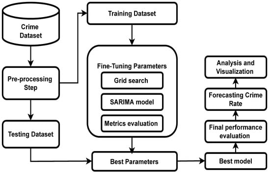
Figure 1. The main steps of the proposed framework.

3.1. Dataset Description

To evaluate our model, a crime dataset was collected from the official website of Saudi Arabia’s government https://data.gov.sa/Data/en/dataset (accessed on 22 October 2022). The dataset contained statistics on crime types, locations, and times of crimes committed. In this study, four types of crimes were examined: robbery, murder, kidnapping, and web crime. In our work, we considered crime datasets for each month as input of our ARIMA model. Table 1 shows a sample of total crimes for each month in Saudi Arabia.

Table 1. Total number sample of crimes for each month in KSA.

Years	Month	Number of Crimes	Date
1419	Muharram	2623	27-04-1998
1419	Safar	3165	26-05-1998
1419	Rabi I	2646	25-06-1998
1419	Rabi II	1875	24-07-1998
1419	Jumada I	2199	23-08-1998
…	…	…	…
1428	Sha’aban	7305	14-08-2007
1428	Rhamadhan	6804	13-09-2007
1428	Shawwal	7471	13-10- 2007
1428	Dhol-Qa’adah	8586	11-11-2007
1428	Dhul-Hijjah	7506	11-12-2007

Figure 2 illustrates a time series plot of monthly KSA from 1998 to 2008. For this study, the real monthly crime data from 1998 to 2004 were used to train the proposed model, and data from 2005 to 2008 were used to evaluate it. Regardless of the fact that this figure depicts the increase and decrease of crime over time, there is no discernible pattern, and the mean of the time series remains constant throughout time, giving the impression that the series has become stationary. The highest crime rate (8586) was reported in the year 2007, while the lowest (1108) was recorded in the year 1999.

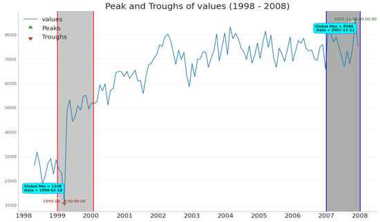
Figure 2. The time series plot of monthly crimes committed in KSA for the years 1990 to 2008.

3.2. Preprocessing

Preprocessing data ensures that the data are prepared in the most meaningful way for a detailed analysis. During the preprocessing step, we cleaned the texts in order to improve the quality of our model. This step involved combining all text values in the comma-separated values (CSV) file and cleaning it by removing duplicate rows. Additionally, the texts were cleaned by removing associated and redundant symbols. Finally, we fed the dataset into our crime analysis model.

3.3. The Autoregressive Integrated Moving Average (ARIMA) Models

ARIMA models offer an additional methodology for the time series forecasting process [24,25]. The two methods that are utilized the most frequently in time series forecasting are exponential smoothing and ARIMA models [26]. These methods offer contrasting approaches to the issue at hand. ARIMA models seek to capture the data’s autocorrelations, as contrasted with exponential smoothing models, which are based on a description of the trend and seasonality in the data. This paper used ARIMA to predict the future crime rate at different times and regions, based on historical data. Hence, the objective of the model was to predict future crimes based on the differences in values in a series instead of using the actual values themselves.

The properties of a time series are said to be stationary if they do not change depending on when the series is observed. Time series that are affected by trends or seasonality are not considered stationary since the trend or seasonality will have an effect on the values of the time series at various points in time. On the other hand, a sequence of white noise is said to be stationary. This means that it does not matter when you watch it; the series should appear to be relatively consistent regardless of the moment in time at which it is viewed. The autoregression AR(p) model is a well-known time series approach for predicting the future value of a series. To do this, data from the p time steps before the current one are utilized as inputs to a regression equation, and those observations are then multiplied by the relevant AR coefficients $\varphi$. In addition, the total is increased by the addition of the mean of the series, denoted by $\mu$, as well as white noise, denoted by $\omega$, which is a random error. The equation below represents the AR(p) model: (1).

$$\mathrm{AR}\left(\mathrm{p}\right):y_t=\mu +\sum _{i=1}^p\left({\varphi }_i{y}_{t-i}\right)+{\omega }_t$$

(1)

Instead of utilizing the previous values of the variable being forecasted in a regression, a moving average model employs past prediction errors to create a model that is similar to a regression. In other words, the moving average MA(q) method is not applicable to any variable in a time series. It is made up of three distinct components, which are as follows: the first variable represents the series’ mean, denoted by $\mu$; a finite number of MA coefficients are added up to give the second variable, denoted by $\theta$, and the model residuals, denoted by $\omega$; and white noise is represented by ${\omega }_t$. The equation that represents the MA(q) model is denoted by Equation (2).

$$\mathrm{MA}\left(\mathrm{q}\right):y_t=\mu +\sum _{i=1}^q\left({\theta }_i{\omega }_{t-i}\right)+{\omega }_t$$

(2)

The ARMA $(p,q)$ model consists of two basic polynomials, denoted by AR(p) and MA(q) [27]. It is described mathematically by Equation (3).

$$y_t=\mu +\sum _{i=1}^p\left({\varphi }_i{y}_{t-i}\right)+\sum _{j=1}^q\left({\theta }_j{\omega }_{t-j}\right)+{\omega }_t$$

(3)

Typically, ARIMA $(p,d,q)$ models are used to analyse and forecast stationary time series [28]. According to Ryabko [29], the fundamental concept behind the ARIMA model is predicated on the assumption that the value that is forecasted for the variable $y_t$ is derived from a linear equation that is constructed of a number of earlier observations that contain random errors. The ARIMA condition $(p,d,q)$ is met by a process $X_t$ when it fulfils Equation (4).

$${\nabla }^d{X}_t={(1-B)}^d{X}_t$$

(4)

3.4. Seasonal ARIMA Model

The seasonal ARIMA $(p,d,q)\times {(P,D,Q)}_s$ model is created by incorporating additional seasonal terms into the ARIMA $(p,d,q)$ models we have seen so far. It is written as shown in Equation (5).

$${\varphi }_p\left(B\right){\Phi }_P\left(B^s\right)W_t={\theta }_q\left(B\right){\Theta }_Q\left(B^s\right){\omega }_t$$

(5)

The following is a description of the notation for Equation (5). The previous equation represents $p,d,$ and q as follows (3): P represents the order of the seasonal AR model, D represents the number of seasonal variations, Q is the order of the seasonal MA, and s is length of the season (periodicity). In addition, the ${\omega }_t$ and B represent the white noise value at period t and the backward shift operator, respectively. Taking into account the relationship between the data, the SARIMA $(p,d,q)times(P,D,Q)s$ model is effectively applied to various time series due to its comparatively small order. Based on the dataset, the period value of the time series s (seasonality) is determined. For example, $s=7,30,365$ for weekly, monthly, and annual data, respectively. d and D specify the order of the nonseasonal and seasonal differencing, and their values cannot exceed 1 and 2, respectively, of the total seasonal difference (i.e., $0\le d,D\le 1$).

Three stages are involved in building an ARIMA model: identification, parameter estimation, and diagnostic testing [30]. The identification of the model involves selecting the appropriate differencing to use to create stationary time series, the desired order of the model, and the autocorrelation (ACF) and partial autocorrelation (PACF) functions that are used to detect the temporal correlation structure of the converted data. When analysing time series data, the ACF may be used to determine if prior values have a specific association with the current values or not. The PACF provides the value of the correlation coefficient between the variable and its time lag for all low-order lags [31].

Both the Akaike’s information criterion and the Bayesian information criterion of Schwarz (BIC) [32] are commonly used methods for selecting optimal models, and they are described in Equations (6) and (7) for AIC and BIC, respectively.

$$\mathrm{AIC}=-2log\left(L\right)+2k=-2log\left(L\right)+2(p+q+P+Q)$$

(6)

$$\mathrm{BIC}=-2log\left(L\right)+kln\left(n\right)=-2log\left(L\right)+(p+q+P+Q)ln\left(n\right)$$

(7)

In this case, n represents a series of observations and k represents a set of ARIMA parameters. We empirically demonstrated that our model became more efficient as the AIC value decreased. It was determined that the model with the lowest AIC score was the best-fitting forecasting model [25].

4. Experimental Evaluation

The results of the experiments are presented in this section, along with the proposed SARIMA model [33,34,35,36,37] and the grid search strategy for selecting the best parameters of the model. A number of experiments were carried out using the data that were gathered from the KSA in order to provide comparative findings utilizing the suggested methodology. In addition, Google Colab was used to conduct the experiments. The findings of the experiments are provided both graphically and in tabular format, and a comparison study with state-of-the art methods is also presented and analysed. The experimental results that were conducted using the proposed approach are reported in the following subsections.

4.1. Experimental Results

Standard libraries such as SciKit Learn and Stat were utilized to perform the experiments. Experiments were carried out using the Google Colab environment, which provided all of the necessary packages. Data were obtained from many official websites. We used KSA data, which were acquired from official data repository websites, to train and verify the proposed SARIMA model. These datasets were from the Kingdom of Saudi Arabia. A grid search was used to fine-tune the many parameters of the proposed model so that it could produce the most accurate forecast. The values of the parameters were determined depending on the data gathered.

The min-max scalar function was utilized in order to perform data normalization. In order to keep the value of variance stable, scaling the data was an essential step. In general, data normalization improves performance and reduces the amount of computing complexity involved. Before beginning to train the model, Equation (8) was used to normalize all of the datasets in this study. In this equation, $X_i$ represents the scaled datasets, $x_i$ refers to the real data, and the terms $min\left(x_i\right)$ and $max\left(x_i\right)$ correspond to the minimum and maximum values of the real dataset.

$$X_i=\frac{x_i-min\left(x_i\right)}{max\left(x_i\right)-min\left(x_i\right)}$$

(8)

Accordion to our experiments, we selected the right forecasting ARIMA approach based on the actual values of the BIC, AIC, RMSE, MAE, and MAPE criteria. Choosing the perfect parameters for ARIMA models using a graphical technique is not a simple or quick process, and it takes a significant amount of time. The grid search (also known as hyperparameter optimization) approach was used to choose the ideal parameter values in a systematic manner. The grid search was used to repeatedly examine alternative combinations of the parameters in different ways. The seasonal ARIMA model was fitted with the SARIMAX() function from the statsmodels module for each combination of parameters, and the evaluation step was done to evaluate the overall quality of the model fit. Once the whole range of parameters had been investigated, then the optimal set of parameters was identified, which was the set of parameters that provided the best performance for the criteria that we were interested in.

A grid search is a hyperparameter optimization approach for determining the best combination of parameter values across several models. The first step in the process of developing any model is to identify a set of parameters and assign a starting value to each one of them. Because we collected data on a monthly basis for a period of 12 months, the value of s was set to 12. After that, a grid search was carried out in order to locate the best possible model with the lowest possible AIC values. The following step was to choose the optimal combination of parameters that would result in the smallest amount of error (AIC) and would then be allocated to the optimal model. The AIC values of several forecasting models are shown in Table 2. Moreover, in Table 2, the lowest AIC value was for the SARIMA $(1,0,8)\times (1,0,0,12)$ model. As a result, the best forecasting model parameter was determined by the combination of parameters $(1,0,8)\times (1,0,0,12)$. In general, the AIC and RMSE values are used to compare SARIMA models. As seen in the comparison table, the SARIMA $(1,0,8)\times (1,0,0,12)$ model’s prediction ability over the forecast period was quite robust when compared with other models. The grid search method solved the problem of determining the optimal parameter values for the proposed SARIMA model.

Table 2. Experimental results for SARIMA models Using Saudi Arabia dataset.

(p, d, q)	(P, D, Q, s)	AIC	MAPE	MAE	MPE	MSE	RMSE	Corr	MinMax
(1, 0, 8)	(1, 0, 0, 12)	−167.9222	0.24716	0.150328	0.237733	0.031013	0.176106	0.530727	0.181175
(1, 0, 8)	(2, 0, 0, 6)	−166.870228	0.233085	0.140898	0.221294	0.028253	0.168086	0.509499	0.171966
(1, 0, 9)	(1, 0, 0, 12)	−166.013507	0.255806	0.155839	0.248155	0.033001	0.181661	0.533153	0.186252
(1, 0, 9)	(2, 0, 0, 6)	−164.987283	0.234343	0.14164	0.223705	0.02858	0.169055	0.519412	0.172596

In a similar manner, Table 3 lists the experimental results for SARIMA models in our dataset with p-values of ≤0.05, which indicated the minimum AIC of each model. Table 3 shows that the SARIMA $(0,0,0)\times (2,0,2,12)$ model had the lowest AIC values. In this study, the best combination of parameters was $(0,0,0)\times (2,0,2,12)$

Table 3. Experimental results of SARIMA models with p-values less than 0.05.

(p, d, q)	(P, D, Q, s)	AIC	MAPE	MAE	MPE	MSE	RMSE	Corr	MinMax
(0, 0, 0)	(2, 0, 2, 12)	−87.482253	0.10098	0.066059	0.071452	0.006327	0.079541	0.853327	0.088572
(0, 0, 2)	(2, 0, 2, 12)	−112.166294	0.139144	0.090887	0.127076	0.011745	0.108376	0.85006	0.116211
(0, 0, 1)	(2, 0, 2, 12)	−102.406443	0.129237	0.081695	0.118656	0.009787	0.098929	0.845524	0.107841
(6, 0, 8)	(0, 1, 2, 12)	−106.470466	0.087934	0.058467	0.033316	0.005926	0.076981	0.84099	0.078726

The real monthly crime data from 1998 to 2008 were split between training and testing datasets in this study. Training data from 1998 to 2004 were used as a training set, and the rest of the data from 2005 to 2008 were used to evaluate the proposed model. Based on the proposed model, high and low confidence limits for actual values for the period 06-08-2005 to 11-12-2007 are shown in Table 4. Based on the previously observed data (Table 4), the proposed model predicted the number of confirmed crimes over the next few days or months with lower and upper confidence limits. Despite the increase in trend, the suggested model performed better on the testing set. The performance of the prediction model was generally satisfactory if the MSE and RMSE values were 0.853327 and 0.088572 for the testing set from 11-01-2008 to 11-03-2009 as shown in Table 5.

Table 4. Experimental results for the proposed SARIMA $(1,0,2)\times (1,0,0,3)$ model (from 6 August 2005 until 11 December 2007) with 95% CI.

Date	Actual	Predicted	Lower	Upper	Date	Actual	Predicted	Lower	Upper
06-08-2005	7445.0	7005.7260	6289.8961	7721.5558	2006-10-23	7485.0	7227.3799	6512.9191	7941.8408
05-09-2005	7196.0	6997.3763	6281.7468	7713.0058	2006-11-22	7590.0	7549.2558	6834.7950	8263.7166
04-10-2005	6894.0	7224.9717	6509.3423	7940.6011	2006-12-22	6582.0	7292.2486	6577.9272	8006.5700
03-11-2005	7364.0	7296.0700	6580.6314	8011.5086	2007-01-20	8190.0	7272.6534	6558.3321	7986.9747
03-12-2005	7893.0	7684.3451	6968.9066	8399.7836	2007-02-19	7994.0	7866.7427	7152.5552	8580.9303
01-01-2006	6896.0	7215.7990	6500.5424	7931.0556	2007-03-20	7697.0	7579.4980	6865.3105	8293.6855
31-01-2006	7311.0	7477.3562	6762.0996	8192.6127	2007-04-18	7893.0	8336.0553	7621.9963	9050.1144
01-03-2006	7745.0	7758.9222	7043.8393	8474.0050	2007-05-18	7483.0	7610.1793	6896.1203	8324.2383
2006-03-30	7643.0	7334.0828	6619.0000	8049.1656	2007-06-16	7060.0	7647.3964	6933.4609	8361.3320
29-04-2006	7838.0	7671.5053	6956.5884	8386.4222	2007-07-15	6682.0	6872.9950	6159.0595	7586.9305
28-05-2006	7409.0	7471.5773	6756.6605	8186.4942	2007-08-14	7305.0	7149.9241	6436.1072	7863.7409
27-06-2006	7328.0	7491.9205	6777.1622	8206.6787	2007-09-13	6804.0	6919.1863	6205.3695	7633.0031
26-07-2006	7355.0	7570.0511	6855.2929	8284.8092	2007-10-13	7471.0	7387.8490	6674.1464	8101.5516
25-08-2006	6994.0	7324.1375	6609.5311	8038.7438	2007-11-11	8586.0	7538.3745	6824.6720	8252.0771
24-09-2006	6930.0	7020.5226	6305.9163	7735.1289	2007-12-11	7506.0	7700.7667	6987.1741	8414.3593

Table 5. Forecasted values of daily confirmed cases for 30 months using a SARIMA $(1,0,2)\times (1,0,0,3)$ model with 95% CI.

Date	Predicted	Lower	Upper	Date	Predicted	Lower	Upper
11-01-2008	8195.778078	7482.185545	8909.370612	2009-04-11	7990.049794	6883.934202	9096.165386
11-02-2008	8475.333189	7688.445969	9262.220409	2009-05-11	7870.693991	6761.046554	8980.341427
11-03-2008	7885.259983	7049.933784	8720.586181	2009-06-11	7905.195620	6791.838300	9018.552939
11-04-2008	8005.299225	7027.213276	8983.385175	2009-07-11	7770.591970	6656.888659	8884.295281
11-05-2008	7676.017299	6684.733328	8667.301271	2009-08-11	7887.609149	6770.468705	9004.749594
11-06-2008	7745.672025	6740.292121	8751.051929	2009-09-11	7823.697939	6706.154293	8941.241584
11-07-2008	7376.689790	6371.191542	8382.188038	2009-10-11	7933.489424	6815.539529	9051.439318
11-08-2008	7660.183727	6642.158550	8678.208904	2009-11-11	8109.932552	6991.573339	9228.291765
11-09-2008	7474.377960	6456.137629	8492.618291	2009-12-11	7960.060314	6841.288690	9078.831938
11-10-2008	7738.974418	6720.517274	8757.431562	2010-01-11	8073.364985	6945.186614	9201.543357
11-11-2008	8176.345989	7157.670361	9195.021618	2010-02-11	8125.719282	6994.248341	9257.190224
11-12-2008	7767.369518	6748.473721	8786.265314	2010-03-11	8048.817954	6914.622189	9183.013718
11-01-2009	8040.837254	6977.589181	9104.085327	2010-04-11	8077.540573	6937.634135	9217.447011
11-02-2009	8156.155368	7081.601112	9230.709624	2010-05-11	8039.500116	6898.074064	9180.926167
11-03-2009	7936.180321	6853.071904	9019.288738	2010-06-11	8060.817630	6917.826242	9203.809017

Figure 3 presents the training set typically expressed in blue from 1998 to 2004, as well as a comparison of the training set and testing set, also represented in blue from 2005 to 2008, and values for the one-step-ahead forecast in red. Additionally, the lower and upper confidence limits for the confidence intervals are denoted by grey shading in the figure.

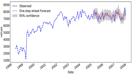
Figure 3. Comparison between the observed and predicted values (one-step-ahead result) for the SARIMA model on a crime dataset.

4.2. Comparison with Other Models

Figure 4 shows the training set, typically represented by a blue line, from 1998 to 2004, as well as a comparison between the testing set, which is also represented by a blue line from 2005 to 2008, and the one-step-ahead forecast, presented by a red line.

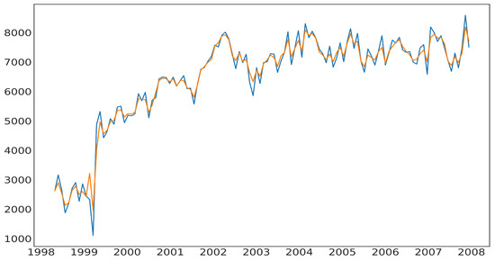
Figure 4. Forecasted values for crime by a random forest model.

Figure 5 demonstrates the training set typically expressed by a blue line from 1998 to 2004, as well as a the forecasted values for crime by a tuned random forest model, and values for one-step-ahead forecast presented by a red line.

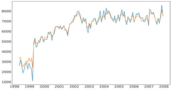
Figure 5. The forecasted values for crime by a tuned random forest model.

Figure 6 shows the forecasted values for crime by an XGB model while Figure 7 shows the plot of the predicted vs. true targets for the crime values by a stacked model as well as a single predictor versus stacked predictors.

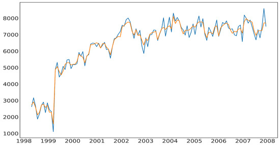
Figure 6. Forecasted values for crime by XGB model.

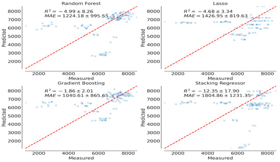
Figure 7. The plot of the predicted vs. true targets for crime values by stacked model.

Table 6 shows the comparison between the current state-of-the-art approaches and the suggested SARIMA model. In Table 6, the random forest model for the KSA data performed much better than the other models in terms of R2 score, while the LR model had an R2 score of 0.60197, indicating that it was statistically less accurate. Additionally, the SARIMA model had an MAE score of 0.066559, which was higher than the other models.

Table 6. A comparison with the state-of-the-art models.

The State-of-the-Art Models	R2 Score	MAE Score
Linear regression (LR)	0.60197	0.899
XGB	0.97907	177.32
Random forest (RF)	0.98187	151.45
SARIMA	0.853	0.066059

5. Conclusions

Previous research was focused on predicting crimes with an accurate and time-efficient method. Previous research are used a prediction model that may produce less accurate results in some cases. In addition, there are a few promising factors that could allow us to predict crime rates with better accuracy. To fill up the gap, we introduced SARIMA model to analysis crime patterns and predict crime in several cities in Saudi Arabia. The dataset in this study was obtained from the Saudi Arabia official websites. It contains information about the crime’s location, type, and date. This study is meant to help the Saudi government understand the distribution of crimes in different cities, predict future crimes and take actions to prevent them. In future research, we will apply the model to many types of crimes, such as robbery, intrusion, and premeditated murder, to improve the model’s performance.

References

- Bahi, A.; Shahidra, K.; Mohd, R.; Zulkifli, Y. Quranic approach in portraying crime stories. Middle East J. Sci. Res. 2012, 12, 124–130. [Google Scholar]
- Adel, H.; Salheen, M.; Mahmoud, R.A. Crime in relation to urban design. Case study: The Greater Cairo Region. Ain Shams Eng. J. 2016, 7, 925–938. [Google Scholar] [CrossRef]
- Ministry of the Interior in Saudi. Statistical Yearbook. 2022. Available online: https://www.moh.gov.sa/en/Ministry/Statistics/book/Pages/default.aspx (accessed on 22 October 2022).
- Kaplan, J. Uniform Crime Reporting (UCR) Program Data: A Practitioner’s Guide. CrimRxiv 2021. [Google Scholar] [CrossRef]
- Bruin, J.D.; Cocx, T.; Kosters, W.; Laros, J.J.; Kok, J. Data Mining Approaches to Criminal Career Analysis. In Proceedings of the Sixth International Conference on Data Mining (ICDM’06), Hong Kong, China, 18–22 December 2006; pp. 171–177. [Google Scholar] [CrossRef]
- Agarwal, J.; Nagpal, R.; Sehgal, R. Crime Analysis using K-Means Clustering. Int. J. Comput. Appl. 2013, 83, 1–4. [Google Scholar] [CrossRef]
- Babakura, A.; Sulaiman, M.N.; Yusuf, M.A. Improved method of classification algorithms for crime prediction. In Proceedings of the 2014 International Symposium on Biometrics and Security Technologies (ISBAST), Kuala Lumpur, Malaysia, 26–27 August 2014; pp. 250–255. [Google Scholar] [CrossRef]
- Yu, C.H.; Ward, M.W.; Morabito, M.; Ding, W. Crime Forecasting Using Data Mining Techniques. In Proceedings of the 2011 IEEE 11th International Conference on Data Mining Workshops, Beijing, China, 8–11 November 2011. [Google Scholar] [CrossRef]
- Almanie, T.; Mirza, R.; Lor, E. Crime Prediction Based on Crime Types and Using Spatial and Temporal Criminal Hotspots. Int. J. Data Min. Knowl. Manag. Process. 2015, 5, 1–19. [Google Scholar] [CrossRef]
- Chen, P.; Yuan, H.; Shu, X. Forecasting Crime Using the ARIMA Model. In Proceedings of the 2008 Fifth International Conference on Fuzzy Systems and Knowledge Discovery, Jinan, China, 18–20 October 2008. [Google Scholar] [CrossRef]
- Sivaranjani, S.; Sivakumari, S.; Aasha, M. Crime prediction and forecasting in Tamilnadu using clustering approaches. In Proceedings of the 2016 International Conference on Emerging Technological Trends (ICETT), Kollam, India, 21–22 October 2016; Volume 50. [Google Scholar] [CrossRef]
- Kim, S.; Joshi, P.; Kalsi, P.S.; Taheri, P. Crime Analysis Through Machine Learning. In Proceedings of the 2018 IEEE 9th Annual Information Technology, Electronics and Mobile Communication Conference (IEMCON), Vancouver, BC, Canada, 1–3 November 2018. [Google Scholar] [CrossRef]
- Borowik, G.; Wawrzyniak, Z.M.; Cichosz, P. Time series analysis for crime forecasting. In Proceedings of the 2018 26th International Conference on Systems Engineering (ICSEng), Sydney, NSW, Australia, 18–20 December 2018. [Google Scholar] [CrossRef]
- Saravanan, M.; Thayyil, R.; Narayanan, S. Enabling Real Time Crime Intelligence Using Mobile GIS and Prediction Methods. In Proceedings of the 2013 European Intelligence and Security Informatics Conference, Washington, DC, USA, 12–14 August 2013; pp. 125–128. [Google Scholar] [CrossRef]
- Pande, V.; Samant, V.; Nair, S. Crime Detection using Data Mining. Int. J. Eng. Res. Technol. 2016, V5, 891–896. [Google Scholar] [CrossRef]
- Butt, U.M.; Letchmunan, S.; Hassan, F.H.; Ali, M.; Baqir, A.; Sherazi, H.H.R. Spatio-Temporal Crime HotSpot Detection and Prediction: A Systematic Literature Review. IEEE Access 2020, 8, 166553–166574. [Google Scholar] [CrossRef]
- Chainey, S.; Ratcliffe, J. Identifying Crime Hotspots. In GIS and Crime Mapping; John Wiley & Sons, Inc.: New York, NY, USA, 2013; pp. 145–182. [Google Scholar] [CrossRef]
- Umair, A.; Sarfraz, M.S.; Ahmad, M.; Habib, U.; Ullah, M.H.; Mazzara, M. Spatiotemporal Analysis of Web News Archives for Crime Prediction. Appl. Sci. 2020, 10, 8220. [Google Scholar] [CrossRef]
- Chackravarthy, S.; Schmitt, S.; Yang, L. Intelligent Crime Anomaly Detection in Smart Cities Using Deep Learning. In Proceedings of the 2018 IEEE 4th International Conference on Collaboration and Internet Computing (CIC), Philadelphia, PA, USA, 18–20 October 2018. [Google Scholar] [CrossRef]
- Azeez, J.; Aravindhar, D.J. Hybrid approach to crime prediction using deep learning. In Proceedings of the 2015 International Conference on Advances in Computing, Communications and Informatics (ICACCI), Kochi, India, 10–13 August 2015; pp. 1701–1710. [Google Scholar] [CrossRef]
- Zhang, Y.; Cheng, T. Graph deep learning model for network-based predictive hotspot mapping of sparse spatio-temporal events. Comput. Environ. Urban Syst. 2020, 79, 101403. [Google Scholar] [CrossRef]
- Wang, B.; Yin, P.; Bertozzi, A.L.; Brantingham, P.J.; Osher, S.J.; Xin, J. Deep Learning for Real-Time Crime Forecasting and Its Ternarization. Chin. Ann. Math. Ser. B 2019, 40, 949–966. [Google Scholar] [CrossRef]
- Shamsuddin, N.H.M.; Ali, N.A.; Alwee, R. An overview on crime prediction methods. In Proceedings of the 2017 6th ICT International Student Project Conference (ICT-ISPC), Johor, Malaysia, 23–24 May 2017; pp. 1–5. [Google Scholar] [CrossRef]
- Paolella, M.S. ARMA Model Identification. In Linear Models and Time-Series Analysis; John Wiley & Sons, Inc.: New York, NY, USA, 2018; pp. 405–442. [Google Scholar] [CrossRef]
- Box, G.E.; Jenkins, G.M.; Reinsel, G.C.; Ljung, G.M. Time Series Analysis: Forecasting and Control; John Wiley & Sons: New York, NY, USA, 2015. [Google Scholar]
- Brockwell, P.J.; Davis, R.A. Introduction to Time Series and Forecasting. Biometrics 1998, 54, 1204. [Google Scholar] [CrossRef]
- Al-Douri, Y.; Hamodi, H.; Lundberg, J. Time Series Forecasting Using a Two-Level Multi-Objective Genetic Algorithm: A Case Study of Maintenance Cost Data for Tunnel Fans. Algorithms 2018, 11, 123. [Google Scholar] [CrossRef]
- Chintalapudi, N.; Battineni, G.; Amenta, F. COVID-19 virus outbreak forecasting of registered and recovered cases after sixty day lockdown in Italy: A data driven model approach. J. Microbiol. Immunol. Infect. 2020, 53, 396–403. [Google Scholar] [CrossRef] [PubMed]
- Ryabko, D. Asymptotic Nonparametric Statistical Analysis of Stationary Time Series; Springer International Publishing: Cham, Switzerland, 2019. [Google Scholar] [CrossRef]
- Eze, N.; Asogwa, O.; Obetta, A.; Ojide, K.; Okonkwo, C. A Time Series Analysis of Federal Budgetary Allocations to Education Sector in Nigeria (1970-2018). Am. J. Appl. Math. Stat. 2020, 8, 1–8. [Google Scholar]
- Rebala, G.; Ravi, A.; Churiwala, S. An Introduction to Machine Learning; Springer International Publishing: Cham, Switzerland, 2019. [Google Scholar] [CrossRef]
- Chen, P.; Niu, A.; Liu, D.; Jiang, W.; Ma, B. Time Series Forecasting of Temperatures using SARIMA: An Example from Nanjing. IOP Conf. Ser. Mater. Sci. Eng. 2018, 394, 052024. [Google Scholar] [CrossRef]
- Malki, A.; Atlam, E.S.; Gad, I. Machine learning approach of detecting anomalies and forecasting time-series of IoT devices. Alex. Eng. J. 2022, 61, 8973–8986. [Google Scholar] [CrossRef]
- Malki, Z.; Atlam, E.S.; Ewis, A.; Dagnew, G.; Ghoneim, O.A.; Mohamed, A.A.; Abdel-Daim, M.M.; Gad, I. The COVID-19 pandemic: Prediction study based on machine learning models. Environ. Sci. Pollut. Res. 2021, 28, 40496–40506. [Google Scholar] [CrossRef] [PubMed]
- Farsi, M.; Hosahalli, D.; Manjunatha, B.; Gad, I.; Atlam, E.S.; Ahmed, A.; Elmarhomy, G.; Elmarhoumy, M.; Ghoneim, O.A. Parallel genetic algorithms for optimizing the SARIMA model for better forecasting of the NCDC weather data. Alex. Eng. J. 2021, 60, 1299–1316. [Google Scholar] [CrossRef]
- Hashim, H.; Atlam, E.S.; Malik Almalki, M.M.E.S.; El-Agamy, R.; Dagnew, G.; Ghoneim, O.; Gad, I. Integrating Data Warehouse and Machine Learning to Predict on COVID-19 Pandemic Empirical Data. J. Theor. Appl. Inf. Technol. 2021, 1, 63–72. [Google Scholar]
- Malki, Z.; Atlam, E.S.; Ewis, A.; Dagnew, G.; Alzighaibi, A.R.; ELmarhomy, G.; Elhosseini, M.A.; Hassanien, A.E.; Gad, I. ARIMA models for predicting the end of COVID-19 pandemic and the risk of second rebound. Neural Comput. Appl. 2020, 33, 2929–2948. [Google Scholar] [CrossRef] [PubMed]
Publisher’s Note: MDPI stays neutral with regard to jurisdictional claims in published maps and institutional affiliations. |
© 2022 by the authors. Licensee MDPI, Basel, Switzerland. This article is an open access article distributed under the terms and conditions of the Creative Commons Attribution (CC BY) license (https://creativecommons.org/licenses/by/4.0/).