Realistic Rendering Algorithm for Bubble Generation and Motion in Water

Abstract

A simplified bubble model and its solver optimization method are proposed to solve the problem of poor realistic simulation and complex solutions for bubble-motion behavior in water. Firstly, the internal velocity of the bubble was avoided, and the bubble model was established by only considering the net flux of the inlet and outlet bubbles, which reduced the computational complexity. The bubble constraint was then introduced into the motion equation of water, and the mixed Euler–Lagrangian method was used to solve it. FLIP particles tracked the bubble position, velocity, and deformation, and the mesh updated the vector field. At the same time, the viscosity term was simplified. Finally, it was combined with implicit incompressible SPH particles to achieve the purpose of volume correction. The experimental results show that the method in this paper can present a simulation effect of bubbles in water with rich detail and a realistic sense, whether compared with actual pictures or with existing methods.

1. Introduction

With the continuous development of computer graphics in fluid simulation, there is a higher requirement for fluid animation, including more artistic visual effects, more accurate flow trends, more efficient calculation methods, and greater micro detail, which brings significant challenges to fluid animation technology based on physics.

Fluid movement in real life usually involves gas. Bubbles are generated due to entrained air flow, whether boiling water, splashing water droplets, or carbonated drinks. If the bubble phenomenon cannot be simulated realistically, the reality of fluid animation is significantly reduced. Where bubbles exist, it represents the coexistence of liquid and gas. However, due to the complexity of bubble motion, the accuracy of detail simulation is relatively high, and the influence of gas on the free surface should also be considered. Bubbles and related two-phase flow phenomena are often ignored in the actual fluid simulation because of the high computational cost. Ideally, one would like to avoid simulating the air or at least drastically reduce the degrees of freedom spent on capturing it. It is standard in bubble simulation to ignore the air and assume a free-surface boundary condition at the interface [1]. However, this treats air as a massless void that collapses when entrained by the liquid because no opposing force is preserving its original volume. Furthermore, water and air differ in density by about three orders of magnitude, making it difficult to solve [2].

Bubbles make the liquid simulation more vivid. In this paper, the Navier–Stokes equation (N–S equation) method is used to simulate the bubble, and the complexity and reality of its calculation are studied.

In order to reduce the computational complexity, based on satisfying the momentum conservation equation of incompressible fluid, and the standard pressure projection, the incompressibility constraint of the bubble is taken as the boundary condition; thus, a simplified model which ignores the change of velocity inside the bubble is established to spare the calculation cost. At the same time, the space segmentation method is used to separate the space in which the particles require retrieving in the form of equidistant grids in the particle neighborhood search phase; only the distance between the space itself and the particles in the adjacent segmentation domain is calculated, which dramatically reduces the calculation time and makes the neighborhood search more efficient.

In enhancing realism, the viscosity coefficient is simplified as a constant extracted in the divergence calculation to correctly represent the vibration deformation of the bubble surface in a low-viscosity liquid. The implicit incompressible Smoothed Particle Hydrodynamics (SPH) particles are generated according to fluid implicit particle (FLIP) interpolation. The pressure quadratic projection is completed by solving the Poisson equation of SPH particles to achieve the purpose of volume correction, which makes the simulation effect of bubbles more realistic and natural.

In summary, the main contributions of this paper are the following:

(1)

A reduced bubble model is established, and a viscous fluid simulation is realized by solving the motion equation with a bubble constraint and viscosity term.

(2)

Bubble tracking and volume correction: each particle is tracked with a unique identifier. The particle identification is used to map the old bubble identifier to the new to form a bipartite graph, which indicates whether the bubble has undergone complex merging and splitting. The volume correction is completed by performing a quadratic pressure projection on the SPH particles generated by interpolation.

2. Related Work

A gas-containing fluid is usually produced in complex fluid scenes. When the fluid flows rapidly and violently, gas will be involved in the fluid. Based on the visual effect, this type of gas material can be divided into large and small-size gas material. We mainly focus on the coupling problem of gas–liquid two-phase flow and simulate the gas phase as the observable bubble in the fluid. Large-size gas materials can show rich gas movement rules. The level set method and SPH method are basically used for bubble modeling and simulation.

As early as 2001, Foster and Fedkiw et al. used the particle level set method to model and simulate bubbles through SPH particles [3], which was well able to simulate bubbles with a resolution lower than a Euler mesh. Greenwood et al. also used the particle level set method to label particles to simulate bubbles but ignored the shape change of the bubbles [4]. At the same time, Song and Zheng et al. used the region level set method to model and simulate large bubbles based on the grid [5,6]. However, this did not successfully simulate bubbles whose shapes were smaller than the size of the established mesh. Kim et al. [7] extended the application of particle level sets in fluid simulation, adding some massless particles, and using the particle system to update their positions when these particles left the host fluid. In 2008, Hong et al. [8] used velocity field to couple the Lagrange and Euler methods to simulate bubbles in water; they used the level set method to simulate deformable bubbles and fluids. At the same time, the Euler method based on the grid was used to capture the movement of water around the bubbles, and gas and liquid were coupled through a velocity field. However, due to the limitation of mesh resolution, it was difficult to simulate the unstable path of foam rising. In 2011, Ihmsen et al. [9] simulated the movement of bubbles and water by the single-phase SPH method, calculated the density and pressure of the gas–liquid two-phase, and then added the tension model to solve the interaction between the two phases. This method solved the problem of a high-density ratio and simulated the complex motion of foam in water. However, the SPH method must ensure a certain distance between particles during initialization. The number of larger-size gas particles is limited by the resolution of fluid particles, which makes the foam less dense. In 2020, Wang Hui et al. [10] proposed a new Eulerian–Lagrangian hybrid method to simulate air bubbles with moving-least-squares (MLS) particles.

It is not difficult to see that the level set method produces a good effect on the phase interface tracking. The SPH method is more suitable for solving fluid motion on a complex surface because it does not rely on the mesh and it avoids the mesh distortion and reconstruction problems caused by the violent fluid movement. Both methods are widely used, but they include several defects.

The level set method continuously leads to the loss of volume due to numerical errors so that the bubbles disappear. Kim and Busaryev et al. chose the volume control method to solve this problem [11,12]. By strengthening the interaction, the correction of the bubble volume resulted in the arrangement and geometry of the bubbles being more in line with the laws of physics. Stomakhin et al. [13] achieved high resolution by only simulating the narrow band around the critical area, while using FLIP particles to conserve bubble volume in water and accurate interface tracking. However, the density at the free surface was misestimated.

Unlike the above method, Hong et al. simulated the bubbles and surrounding liquid as a multiphase flow [14] and combined the volume of fluid (VOF) and front tracking method to track the bubble surface. Thürey et al. coupled the particle system with the two-dimensional shallow-water model to simulate the motion of bubbles and water bodies and to calculate the flow field around bubbles with the experimental curl potential function [15]. Cleary et al. [16] used the gas-diffusion equation to simulate nucleation bubbles generated by gas dissolution. Discrete spheres with fixed shapes modeled bubbles. The coupling between gas materials and liquids was realized by a drag force, while the influence of gas materials on the liquid was ignored. In 2012, Shao et al. [17] proposed a gas material generation model considering gas concentration and solid–liquid velocity difference. When a gas particle on the surface of a rigid body is regarded as a virtual nucleation point, the gas particle will absorb gas from the surrounding liquid and become an observable foam. In 2015, Ando et al. proposed a stream function model solver to calculate complex bubble formation without explicitly solving the gas phase [18]. Aanjaneya [19] developed an efficient solver to accelerate fluid-structure coupling and improve calculation efficiency. In 2020, Ishida et al. [20] took into account the thickness of the gas-particle film and realistically realized the simulation of single foam deformation and multifoam collapse and fusion phenomena. Liu Sinuo et al. [21] suggested a multi-scale gas simulation method in liquid under the unified particle framework to simulate gas particles with different radii and their coupling process with liquid particles, which avoided the instability caused by random initialization. Luan et al. [22] presented a novel velocity transport technology for two individual particles based on the affine particle-in-cell (APIC) method to solve the instability problem caused by fluid-implicit particles and effectively realized the simulation of a two-phase fluid.

Minor errors and incompressibility in surface tracking inevitably lead to volume changes in liquid simulation. Regarding volume correction, Kim et al. [11] first proposed using divergent sources to recover the lost volume. The particle-based model introduced direct particle position and density correction [23,24,25]. In the context of mesh-based surface tracking, Langlois et al. used scalar fields to track the identity and volume of bubbles so that their volumes could be used to synthesize physical-based bubble sounds [26]. However, the method did not describe how to redistribute the volume, mainly when multiple topological changes coincided in nearby bubbles. Chen et al. [27] proposed an extended-cut grid method to deal with liquid structures with a lower surface tension than grid elements.

Targeting the high computational cost of bubbles in water, we propose a bubble simulation method which simplifies the viscosity term in the motion equation, uses marker and cell (MAC) mesh to capture bubbles and liquids, and strives to simulate bubbles in water as accurately as possible. At the same time, by interpolating FLIP particles, implicit incompressible SPH particles are generated for secondary pressure projection to correct the bubble volume.

3. Bubble Modeling

3.1. Simplified Bubble Model

Gases in liquids are usually of different sizes, and visible air masses are regarded as large-size gas materials. When modeling large-size gas particles, the fluid is usually regarded as a gas–liquid two-phase fluid, and a complex physical model including buoyancy and resistance is established. This model can vividly describe the shape change of a bubble, but the calculation process is very time-consuming.

It is well known that air is much lighter than water and cannot usually transfer much momentum to water, but it still has the constraint of incompressibility: bubbles in water retain their volume to a large extent. Therefore, we set the mass of the bubble to be zero, so its momentum can be ignored, and only the net flow into and out of each bubble is considered. Thus, a simplified model that ignores the velocity change inside the bubble is established, saving computational costs. The schematic diagram of the simulation area is shown in Figure 1.

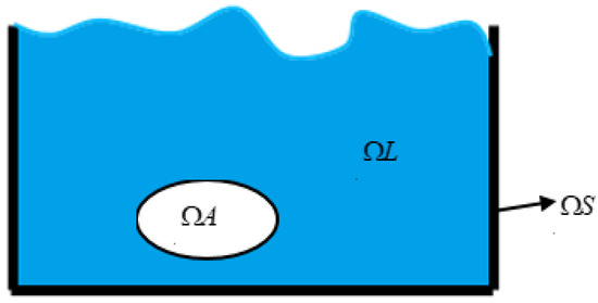
Figure 1. Schematic diagram of the simulation area.

To maintain the volume of each bubble, for the $i$th bubble, we have

$${\displaystyle \underset{\partial \mathsf{\Omega }{A}_i}{\iint }\mathit{u}•\mathit{n}dA}=0$$

(1)

where $\partial \mathsf{\Omega }{A}_i$ is the $i$th bubble region and its surface, and u is the velocity of the incompressible liquid.

Formula (1) can be divided into two liquid and solid parts:

$$\left\{\begin{array}{c}{B}_i\mathit{u}={\displaystyle \sum _{\mathsf{\Omega }L\cap \partial {\mathsf{\Omega }}_{A_i}}\mathit{u}•{\mathbf{n}}_{f}d{\mathrm{A}}_f}\\ b_{S_i}={\displaystyle \sum _{\mathsf{\Omega }S\cap \partial {\mathsf{\Omega }}_{A_i}}{\mathit{u}}_S•{\mathbf{n}}_{f}d{\mathrm{A}}_f}\end{array}\right.$$

(2)

where $\mathsf{\Omega }L$ is the liquid region, $\mathsf{\Omega }S$ is the solid region, and $B_i$ is a row vector representing the discretization of the i-th bubble constraint, summing the net flow through the bubble incident liquid surface. Similarly, the solid contribution is expressed as $b_{S_i}$, ${\mathbf{n}}_f$ is the unit face-normal oriented outside the bubble area, and ${\mathrm{A}}_f$ refers to the area of the associated face.

3.2. Solution of Motion Equation

In this paper, the fluid momentum equation under incompressible conditions is considered

$$\frac{D\mathit{u}}{Dt}=g-\frac{1}{\rho }\nabla p$$

(3)

Here $\rho$ is the liquid density and p is the liquid pressure.

All bubble constraints are represented by a matrix B, and the constraint conditions are associated with the pressure term; the partial differential equation is obtained as follows:

$$\begin{array}{c}\rho \frac{\partial \mathit{u}}{\partial t}=-\nabla p-\frac{\partial B^T}{\partial \mathit{u}}\lambda ,\\ \nabla •\mathit{u}=0,\\ B\mathit{u}=-b_S\end{array}$$

(4)

where $\lambda$ is a Lagrange multiplier assigned to each bubble.

When the FLIP method is used to solve the problem, the pressure and velocity of FLIP particles are first interpolated into the grid, and then solved on the grid. The increment of these physical attributes is then interpolated back to the particles to update the particle attributes.

These are directly discretized on the standard MAC grid. As shown in Figure 2, the MAC grid is a cross-arranged grid divided based on spatial coordinates. The grid and liquid are independent, and different physical quantities are stored in different grid positions. The center of the grid stores the fluid pressure value, and the edge part stores the fluid velocity field vector in a staggered order. The tracing of the liquid interface is shown in Figure 3. The lattice with liquid is marked L, the lattice with a solid boundary is marked S, and the air area is marked A. These grids form the shape of the liquid surface. In the calculation process, velocity and pressure are the main variables of the flow field. The pressure and velocity fields of fluid motion are obtained by solving the continuous equation for a viscous incompressible fluid.

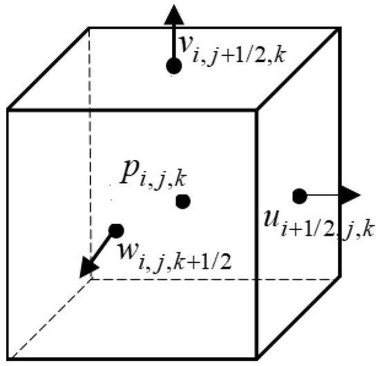
Figure 2. MAC mesh structure.

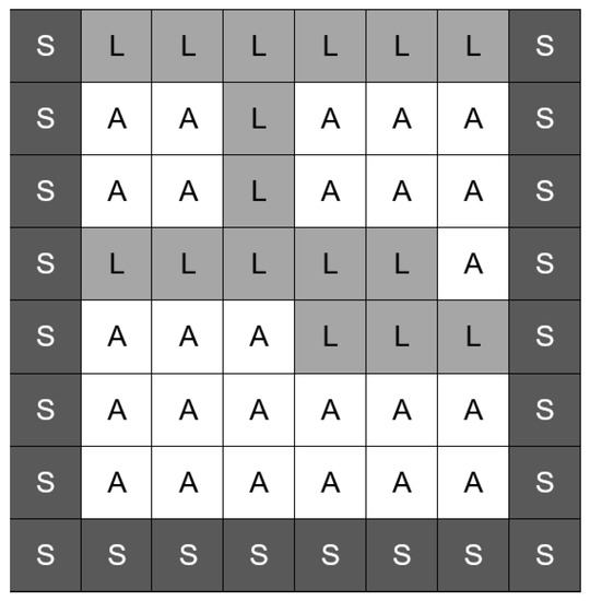
Figure 3. Marker grid 2D example.

3.3. Viscous Fluid Simulation

The appearance of a viscous force reduces the bubble velocity and has a non-negligible effect on the bubble shape. After solving the linear system of p and $\lambda$, the influence of the viscosity term on velocity is solved.

The momentum equation of a viscous liquid is as follows:

$$\frac{D\mathit{u}}{Dt}=-\frac{1}{\rho }\nabla p+\frac{1}{\rho }\nabla •(\mu (\nabla \mathit{u}+\nabla {\mathit{u}}^T))$$

(5)

Generally, the simulation of bubbles in highly viscous liquids is not considered. In order to reduce the computational complexity, in this paper, the above formula is simplified. For simulation scenarios with a constant viscosity, that is, when $\mu$ is constant, the viscosity term can be removed from the divergence calculation, and Formula (5) is expressed as

$$\begin{array}{ll}\hfill \frac{D\mathit{u}}{Dt}& =-\frac{1}{\rho }\nabla p+\frac{\mu }{\rho }\nabla •(\nabla \mathit{u}+\nabla {\mathit{u}}^T)\\ & \mathbf{=}-\frac{1}{\rho }\nabla p+\frac{\mu }{\rho }[\nabla •\nabla \mathit{u}+\nabla •(\nabla {\mathit{u}}^T)]\end{array}$$

(6)

The results are as follows:

$$\frac{D\mathit{u}}{Dt}=-\frac{1}{\rho }\nabla p+\frac{\mu }{\rho }[\nabla •\nabla \mathit{u}+\nabla (\nabla •\mathit{u}))]$$

(7)

and the liquid is incompressible, that is $\nabla •\mathit{u}$ = 0. Finally, if the kinematic viscosity $\nu =\frac{\mu }{\rho }$ is substituted, the viscosity term is expressed as $\nu {\nabla }^2\mathit{u}$.

Either the explicit or implicit method can be used to solve the viscosity term in the grid. If the forward Euler method is directly used to calculate the viscosity term at the current velocity u, the change of the velocity field can be directly calculated at each time step. The central difference is used as the difference scheme of the Laplace operator

$$\begin{array}{cc}{\nabla }^2{\mathit{u}}^n& =L({\mathit{u}}^n)\hfill \\ & =\frac{{\mathit{u}}_{i+1}-2{\mathit{u}}_i+{\mathit{u}}_{i-1}}{\mathsf{\Delta }{x}^2}i\hfill \\ & +\frac{{\mathit{u}}_{j+1}-2{\mathit{u}}_j+{\mathit{u}}_{j-1}}{\mathsf{\Delta }{y}^2}j\hfill \\ & +\frac{{\mathit{u}}_{k+1}-2{\mathit{u}}_k+{\mathit{u}}_{k-1}}{\mathsf{\Delta }{z}^2}k\hfill \end{array}$$

(8)

The stability conditions are as follows:

$$\frac{12\mathsf{\Delta }t\nu }{\mathsf{\Delta }{x}^2}<1$$

It is not difficult to see that this method is strictly limited by step size and will cause unstable diffusion solution if the accuracy is insufficient.

In this paper, the backward Euler iterative equation is used to obtain:

$${\mathit{u}}^{n+1}={\mathit{u}}^n+\mathsf{\Delta }t\nu {\nabla }^2{\mathit{u}}^n$$

(9)

The equation is a linear equation system, which is solved similarly to the pressure term. The conjugate gradient descent method is used to solve linear equations, and the bubble motion in liquids with different viscosities can be simulated by controlling the input of different viscosity coefficients.

The pressure solution is forced on the free surface $p=0$. At the solid boundary $\mathit{u}•n={\mathit{u}}_S•n$. The no-slip boundary condition is used to solve the viscosity term.

4. Bubble Tracking

Having built the physical model for simulating the bubble, reducing the bubble volume drift is the next significant difficulty. Due to the instability of bubble shape, the complexity of motion, and the uncertainty of a moving object’s position, it is incredibly complex to correctly simulate bubble tracking.

Previous bubble simulation methods mostly used the level set or particle methods to directly track liquid and bubble regions. This paper extends the primary FLIP method by simply labeling any non-solid or non-liquid region as a bubble. However, it is well known that cumulative numerical advection errors can cause liquid FLIP particles to separate or aggregate over time, resulting in erroneous volume changes and occasionally creating false space gaps or voids. Since we do not explicitly track the geometry of the air, the liquid volume drift destructively modifies the implied bubble volume, while the artificial void produces false bubbles that begin to rise. Precise tracking of the bubble material can prevent voids, reduce volume changes to some extent, and add additional overhead. In order to solve these problems, we implicitly tracked bubbles by adding bubble ID attributes to each FLIP particle.

We used the old bubble ID stored on the FLIP particles in the previous step and the bubble ID assigned to the new bubble regions to build a bubble ID map from the previous time step to the next time step. As shown in Figure 4, the particle was initially assigned its adjacent bubble ID, and after advection, the particle ID was used to map the old bubble ID to the new bubble ID. The mapping forms a bipartite graph in which uppercase letters represent the old bubble regions, lowercase letters represent the new bubble regions in the next step, and edges indicate whether the bubbles are simply advected or have undergone more complex mergers and splits.

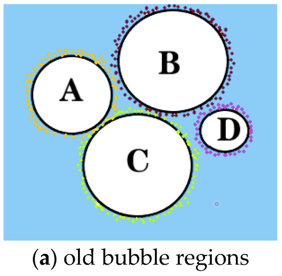
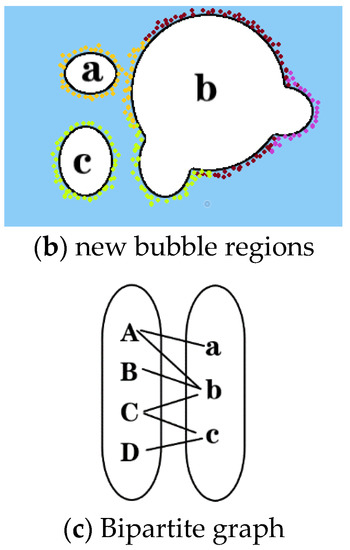
Figure 4. Bubble ID mapping legend.

Using this mapping, the bubbles generated without reason correspond to the new bubble ID node with no edges introduced. They can be disintegrated by applying negative divergence. The volume change of the bubble is related to its divergence.

$${\displaystyle \underset{{\mathsf{\Omega }}_B}{\int }\nabla \cdot \mathit{u}\approx \frac{v_B^{n+1}-v_B^n}{\mathsf{\Delta }t}}$$

(10)

Here bubble collapse is driven by setting $v_B^{n+1}=0$.

5. Correction for Bubble Volume

5.1. Generation of SPH Particles

Although it is a standard simplified method to solve the viscosity term from pressure projection, it undoubtedly increases the divergence and the effect of volume drift. Therefore, a second pressure projection is required before the advection of the velocity field is continued.

Instead of directly repeating the previous pressure projection step on the mesh, the volume correction is realized by combining FLIP particles with implicit incompressible SPH (IISPH) particles to solve the Poisson equation with a constant density as the source term.

Eight FLIP particles are interpolated in each time step to generate one SPH particle. A Kernel function is used to interpolate FLIP particle velocity u to initialize SPH particle velocity.

$${\mathit{u}}_p=\frac{{\displaystyle \sum \mathit{u}W}}{{\displaystyle \sum W}}$$

(11)

The kernel function $W=W(‖x_i-x_j‖,2h)$, where $x_i$ and $x_{\mathrm{j}}$ are the positions of these two particles, and $h$ is the distance between SPH particles.

The pressure Poisson equation is as follows:

$${\nabla }^{2}p=\frac{{\rho }_0-{\rho }^{n+1}}{\mathsf{\Delta }{t}^2}$$

(12)

After discretization, solving of p updates ${\mathit{u}}_p$, and corrects the density change due to divergence to a static density.

Next, we interpolate the SPH particle’s velocity back to the flip particle:

$${\mathit{u}}^{*}=\mathit{u}+\frac{{\displaystyle \sum {\mathit{u}}_p(\mathrm{t}+\mathsf{\Delta }\mathrm{t})-{\mathit{u}}_{p}W}}{{\displaystyle \sum W}}$$

(13)

5.2. Hybrid Particle Implementation of Flip

SPH is usually affected by numerical diffusion, especially in low-resolution simulation. FLIP particles help to maintain vorticity and add detail to SPH particles. Therefore, this paper uses a combination of Z-index sorting and compact hashing to accelerate the neighborhood search. This paper briefly introduces how to optimize the neighborhood search in the framework and improve the simulation efficiency and effect by selecting the appropriate acceleration structure.

All FLIP and SPH particles are stored in the same uniform mesh, with a side length of r = 2 h, because the same cubic spline kernel is used in IISPH with the support being 2 h, used for the velocity interpolation between the FLIP and SPH particles. Before the pressure calculation, the adjacent FLIP and SPH particles are queried for each SPH particle.

The efficiency of neighborhood search contributes to the computational cost of the simulation for SPH particle simulation. The related optimization acceleration is, therefore, essential to the research of neighborhood search methods.

Generally, a method based on the regular grid is conducted to accelerate the search. As shown in Figure 5, the current search radius is h, and the length of a standard grid is r. The position information of the specified particle i can be determined by searching ${\left(\frac{2h}{r}+1\right)}^3+1$ grids. The advantage of the regular grid is that it is simple to implement, and the time complexity of the neighborhood search is constant in an ideal case.

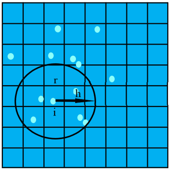
Figure 5. Schematic diagram of particle search based on Grid.

6. Bubble and Rendering of Water Environment

For the effect that the middle transparency of the bubble in water is higher than the surrounding transparency, we can check the angle between the line of sight and the normal vector of the bubble patch.

Firstly, it is processed in the vertex shader. In the vertex shader, vertex coordinates and normal vectors are transformed into the world, the viewpoint, and the projection without special operation. The processed data are then interpolated into the Fragment Shader for processing. Here, the lighting calculation is performed first, and the Blinn–Phong model is used to calculate the color of the diffuse and specular reflections of the bubbles. The alpha value for alpha blending the pixels with the background is then determined. In order to achieve the effect that the transparency in the middle of the bubble is higher than that of the surrounding transparency, we first calculate the angle between the line of sight and the normal vector

$$\cos \theta =\left|\left(n_c\cdot \nu \right)\right|$$

(14)

In fact, what is calculated here is the cosine value of the included angle, but this value is retained for the convenience of calculating the alpha value in the future. In Formula (14), $n_{\mathrm{c}}$ is the normal vector of the pixel in the camera coordinate system, and $\nu$ is the line of sight direction in the camera coordinate system (i.e., the vector (0,0,1) pointing to the inside of the screen).

As shown in Figure 6, the opacity of the bubble is related to the angle between its normal vector and the line of sight. Only the opacity of the positive face is calculated here. The larger the absolute cosine value of the included angle, the greater the pixel’s opacity. On the contrary, the smaller the absolute cosine value of the included angle, the lower the opacity. Therefore, we set the Alpha value of the pixel to:

$$Alpha=1-\cos \theta$$

(15)

to achieve the desired effect.

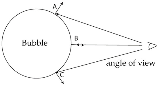
Figure 6. Calculation Schematic.

The rendering of the water body is similar to that of bubbles, except that there is no effect of the intermediate transparency being higher than the surrounding transparency. In the rendering, a simple Blinn–Phong model calculates the lighting, and Alpha Blending is used for blending.

7. Results

The system environment was a Windows 10 (64-bit) operating system. C++ programming language and Cg shading language were used for programming on the Houdini 3D computer graphics platform and supplemented by Autodesk 3ds Max for modeling, to achieve the simulation of complex bubble motion phenomenon, namely the dynamic tracking simulation of bubbles. The hardware development platform used in this system was an Intel (R) core (TM) i7-8550u CPU @ 1.80 GHz, 1.99 GHz, 8g RAM, and the graphics card was an NVIDIA GeForce MX150.

7.1. Experimental Design

The experiments in this paper were designed from three aspects: bubble modeling, the underwater bubble motion process, and the large-size bubble effect. The experiment was divided into five groups. The first group of experiments aimed to show the effect of the bubble model after the booming construction. The second group of experiments shows the bubble generation process in a straw. The third group of experiments show the bubble movement process after the viscosity term was added. The fourth group of experiments show the bubble effect under different viscosity coefficients. The fifth group of experiments aimed to show the generation effect of large-scale bubbles. The algorithm simulated the five groups of experiments in this paper, and the results were compared to the real bubble or the current mainstream bubble simulation methods.

Experiment 1. Figure 7 shows the bubble generation process at the bottom of a container. The initial shape of the bubble is spherical because the Lagrange multiplier assigned when modeling the bubble is equivalent to a constant pressure value inside the bubble, and the initial shape is the result of the balance between the internal pressure of the gas and the internal pressure of the liquid. The fluid viscosity and inertia deform the bubble in the following upward motion.

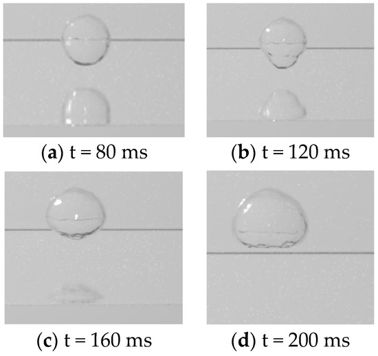
Figure 7. Bubble generation effect of the method in this paper.

Figure 7 shows the effects of upward motion at different times after bubble generation. Figure 7a shows the bubbles generated after 80 ms, Figure 7b reveals the bubbles generated after 120 ms, Figure 7c displays the bubbles generated after 160 ms, and Figure 7d indicates the bubbles generated after 200 ms. The objects similar to bubbles in Figure 7a–c below are bubble reflection images, which gradually decrease as the bubbles rise. Due to the constant change of internal and external pressure, the bubble no longer maintains a spherical shape and exhibits a certain degree of deformation when it rises continuously.

Experiment 2. Figure 8a shows the bubble generation process in a straw, captured by mobile phone video. Figure 8b shows the bubble in the water generated by the algorithm in this paper.

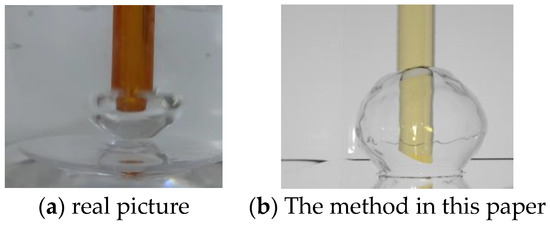
Figure 8. Comparison of the effectiveness of the bubble model.

The bubble in the water is super bright because it is surrounded by a circle of total internal reflection (TIR) with a perfect reflection. The rendering of bubbles in water should be achieved by assigning the bubble geometry higher priority than water and the straw index of refraction inside the bubble. Thus, the refraction effect of light at different boundaries between air, liquid, and glass can be correctly reflected. The experiment demonstrates that our method provides a visually credible bubble effect in water.

Experiment 3. Figure 9 shows the picture of a real bubble, reference [28], reference [23], and this paper on bubble motion. As shown in Figure 9a, the overall shape of the real-world bubble in a low-viscosity liquid is elliptical, and the bottom surface is concave inside, forming a typical bubble jet. As shown in Figure 9b, reference [28] solves the typical Euler equation without considering the viscosity term, so the deformation of a bubble in motion cannot be correctly expressed. As shown in Figure 9c, reference [23] adopts the simulation method of extended particle level set, which can show the complex scene of multiphase flow including bubbles, but it also aggravates the volume loss in the original particle level set method. Figure 9d shows the simplified incompressible viscous fluid model proposed in this paper; this achieves a more realistic bubble motion than the simulation results in references [23,28].

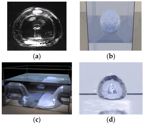
Figure 9. Comparison of the bubble movement effect of real picture with the three methods. (a) real picture, (b) reference [28], (c) reference [23], (d) this paper.

Experiment 4. Figure 10 shows the bubble effect under different dynamic viscosity coefficients. The viscous force of the liquid hinders the upward movement of the bubble, and the bubble transforms from a spherical shape to an ellipsoid shape. Except for the jet generated on the lower surface due to inertia and viscous force, the surface is subject to a slight oscillation deformation. It can be observed that the larger the dynamic viscosity coefficient, the greater the surface deformation.

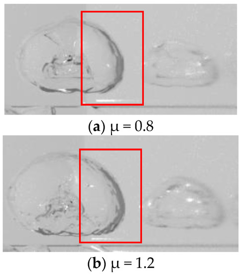
Figure 10. Comparison of different viscosity coefficients.

There are more complex and large-scale bubble movements in natural scenes, such as boiling water, a propeller rotating at high speed in the water, gas generated by the underwater explosion, and so on. In order to ensure the realization of real complex motions in nature, a set of comparative experiments were designed to verify the correctness of the proposed theory.

Experiment 5. Figure 11 shows the effects of references [11,29], and this paper on the generation of large-scale bubbles in the water. Reference [11] used the level set method to track the free surface, and divergence was used as the control variable. Although the volume was well maintained, the bubble deformation is unnatural, which is inconsistent with the actual situation. Reference [29] used SPH particles and a new bubble model, but an abnormal phenomenon arises, in that the water particles with high velocity pass through the bubble particles in the simulation. Based on the consideration of the viscosity term, the implicit incompressible SPH particles were generated by interpolation to correct the volume. Figure 11c shows the particle form diagram simulating the large-scale bubbles generation process in a water tank, and Figure 11d is the rendered result, which is more realistic and natural than those in references [11,29].

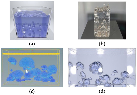
Figure 11. Comparison of generation effects of large-scale bubbles. (a) Reference [11], (b) Reference [29], (c) This paper (in particle form), (d) This paper (after rendering).

The method in this paper simulates the movement process of large-sized bubbles with visible shapes in a liquid and achieves an accurate and effective simulation effect. In order to further verify the applicability of our method, we also designed an experiment to simulate the movement process of small-scale gas materials.

Experiment 6. Figure 12 shows the generation process of bubbles at the bottom of a wine glass. Bubbles were generated with the pouring of liquid. Because they are tiny and dense bubbles, the shape is a standard spherical shape. By setting the priorities for glass material, liquid material, and bubble shader, the refraction of light can be correctly reflected, making the scene more realistic and natural.

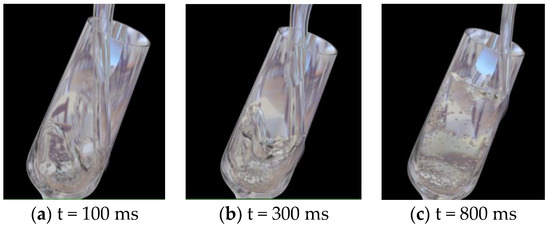
Figure 12. Small-size bubble renderings.

7.2. Program Efficiency

Table 1 lists the parameters of each scene implemented by the method in this paper. The number of particles is the total number of FLIP particles. The experimental data show that the proposed method can fully meet the needs of bubble-motion simulation in water under large-scale particle numbers.

Table 1. Experimental data for different experimental scenarios.

Scenes	Dynamic Viscosity Coefficient μ (Centipoise cP)	Number of Particles	Solver Solution Time	$\mathbf{SPH} \mathbf{Particle} \mathbf{Spacing} \mathit{h}$	Frames/s (FPS)
Bubble generation (Figure 7)	0.8	1.4 × 106	8 h	0.925	25
Generated in bubble pipette (Figure 8b)	0.8	1.6 × 106	8 h	0.925	24
Bubble movement effect (Figure 9d)	1	2.2 × 106	25 h	1.5	24
Bubble movement effect (Figure 10a)	0.8	1.5 × 106	10 h	1	24
Bubble movement effect (Figure 10b)	1.2	1.6 × 106	11 h	1	24
Massive bubbles (Figure 11)	1	2.2 × 106	48 h	1.85	22

8. Conclusions

This paper proposes an optimization method for the bubble model and its solver. The viscosity term is considered in the solution of the momentum equation, and it is simplified to a certain extent, and the backward Euler method is used to solve it after the pressure projection. By interpolating FLIP particles to generate incompressible implicit SPH particles and using the secondary projection of new particles on pressure to maintain bubble volume, the accuracy of the simulation is improved, and the problem that bubbles in water cannot be correctly deformed is successfully solved. The motion effect of typical bubbles is realized, and the realism of underwater bubble-motion behavior is significantly improved.

The method in this paper can effectively simulate the formation and movement of large-size bubbles in water. However, the simulation effect of the extremely unstable free surface caused by bubbles requires improvement and the accurate solution of the viscosity term also requires further study. In future work, we will continue to expand our research on the basis of the method in this paper to simulate the behavior of a more abundant multiphase flow in a real and stable way.

References

- Bridson, R. Fluid Simulation for Computer Graphics; CRC Press: Boca Raton, FL, USA, 2015. [Google Scholar]
- Maclachlan, S.P.; Tang, J.M.; Vuik, C. Fast and robust solvers for pressure-correction in bubbly flow problems. J. Comput. Phys. 2008, 227, 9742–9761. [Google Scholar] [CrossRef]
- Foster, N.; Fedkiw, R. Practical animation of liquids. In Proceedings of the 28th Annual Conference on Computer Graphics and Interactive Techniques, Los Angeles, CA, USA, 12–17 August 2001; ACM Press: New York, NY, USA, 2001; pp. 23–30. [Google Scholar]
- Greenwood, S.T.; House, D.H. Better with bubbles: Enhancing the visual realism of simulated fluid. In Proceedings of the 2004 ACM SIGGRAPH/Eurographics Sympo-Sium on Computer Animation, Grenoble, France, 27–29 August 2004. [Google Scholar]
- Song, O.Y.; Shin, H.; Ko, H.S. Stable but nondissipative water. ACM Trans. Graph. 2005, 24, 81–97. [Google Scholar] [CrossRef]
- Zheng, W.; Yong, J.H.; Paul, J.C. Simulation of bubbles. In Proceedings of the 2006 ACM SIGGRAPH/Eurographics sympo-sium on Computer animation, Vienna, Austria, 2–4 September 2006; Eurographics Association: Vienna, Austria, 2006; pp. 325–333. [Google Scholar]
- Kim, J.; Cha, D.; Chang, B. Practical animation of turbulent splashing water. In Proceedings of the ACM SIGGRAPH/Eurographics Symposium on Computer Animation, Vienna, Austria, 2–4 September 2006; ACM Press: New York, NY, USA, 2006; pp. 335–344. [Google Scholar]
- Hong, J.M.; Lee, H.Y.; Yoon, J.C.; Kim, C.-H. Bubbles alive. ACM Trans. Graph. 2008, 27, 48. [Google Scholar] [CrossRef]
- Ihmsen, M.; Bader, J.; Akinci, G.; Teschner, M. Animation of Air Bubbles with SPH. GRAPP 2011, 11, 225–234. [Google Scholar]
- Wang, H.; Jin, Y.; Luo, A.; Yang, X.; Zhu, B. Codimensional surface tension flow using moving-least-squares particles. ACM Trans. Graph. 2020, 39, 42:1–42:14. [Google Scholar] [CrossRef]
- Kim, B.; Liu, Y.; Llamas, I.; Jiao, X.; Rossignac, J. Simulation of bubbles in foam with the volume control method. ACM Trans. Graph. 2007, 26, 98.1–98.10. [Google Scholar] [CrossRef]
- Busaryev, O.; Dey, T.K.; Wang, H.; Ren, Z. Animating bubble interactions in a liquid foam. ACM Trans. Graph. 2012, 31, 1–8. [Google Scholar] [CrossRef]
- Stomakhin, A.; Wretborn, J.; Blom, K.; Daviet, G. Underwater bubbles and coupling. In Proceedings of the SIGGRAPH ’20: Special Interest Group on Computer Graphics and Interactive Techniques Conference, Washington, DC, USA, 19–23 July 2020. [Google Scholar]
- Hong, J.M.; Kim, C.H. Animation of Bubbles in Liquid. Comput. Graph. Forum 2003, 22, 253–262. [Google Scholar] [CrossRef]
- Thürey, N.; Sadlo, F.; Schirm, S.; Gross, M. Real-time simulations of bubbles and foam within a shallow-water framework. In Proceedings of the ACM Siggraph/Eurographics Symposium on Computer Animation, San Diego, CA, USA, 3–4 August 2007. [Google Scholar]
- Cleary, P.W.; Pyo, S.H.; Prakash, M.; Koo, B.K. Bubbling and frothing liquids. ACM Trans. Graph. 2007, 26, 97. [Google Scholar] [CrossRef]
- Shao, X.; Zhou, Z.; Wu, W. Particle-based simulation of bubbles in water-solid interaction. Comput. Animat. Virtual Worlds 2012, 23, 477–487. [Google Scholar] [CrossRef]
- Ando, R.; Thuerey, N.; Wojtan, C. A stream function solver for liquid simulations. ACM Trans. Graph. 2015, 34, 1–9. [Google Scholar] [CrossRef]
- Aanjaneya, M. An Efficient Solver for Two-way Coupling Rigid Bodies with Incompressible Flow. Comput. Graph. Forum 2018, 37, 59–68. [Google Scholar] [CrossRef]
- Ishida, S.; Synak, P.; Narita, F.; Hachisuka, T.; Wojtan, C. A model for soap film dynamics with evolving thickness. ACM Trans. Graph. 2020, 39, 31:1–31:11. [Google Scholar] [CrossRef]
- Liu, S.; Wang, B.; Ban, X. Multiple-scale Simulation Method for Liquid with Trapped Air under Particle-based Framework. In Proceedings of the 2020 IEEE Conference on Virtual Reality and 3D User Interfaces (VR), Atlanta, GA, USA, 22–26 March 2020; pp. 842–850. [Google Scholar]
- Lyu, L.; Cao, W.; Wu, E.; Yang, Z. Affine particle-in-cell method for two-phase liquid simulation. Virtual Real. Intell. Hardw. 2021, 3, 105–117. [Google Scholar] [CrossRef]
- Losasso, F.; Shinar, T.; Selle, A.; Fedkiw, R. Multiple interacting liquids. ACM Trans. Graph. 2006, 25, 812–819. [Google Scholar] [CrossRef]
- Kugelstadt, T.; Longva, A.; Thuerey, N.; Bender, J. Implicit density projection for volume conserving liquids. IEEE Trans. Vis. Comput. Graph. 2019, 27, 2385–2395. [Google Scholar] [CrossRef] [PubMed]
- Takahashi, T.; Lin, M.C. A Geometrically Consistent Viscous Fluid Solver with Two-Way Fluid-Solid Coupling. Comput. Graph. Forum 2019, 38, 49–58. [Google Scholar] [CrossRef]
- Langlois, T.R.; Zheng, C.; James, D.L. Toward animating water with complex acoustic bubbles. ACM Trans. Graph. 2016, 35, 95. [Google Scholar] [CrossRef]
- Chen, Y.L.; Meier, J.; Solenthaler, B.; Azevedo, V. An extended cut-cell method for sub-grid liquids tracking with surface tension. ACM Trans. Graph. 2020, 39, 1–13. [Google Scholar] [CrossRef]
- Goldade, R.; Aanianeya, M.; Batty, C. Constraint bubbles and affine regions: Reduced fluid models for efficient immersed bubbles and flexible spatial coarsening. ACM Trans. Graph. 2020, 39, 43:1–43:15. [Google Scholar] [CrossRef]
- Gu, Y.; Yang, Y.H. Physics based boiling bubble simulation. In Proceedings of the SIGGRAPH ASIA 2016 Technical Briefs, Macao, China, 5–8 December 2016; pp. 1–4. [Google Scholar]
Publisher’s Note: MDPI stays neutral with regard to jurisdictional claims in published maps and institutional affiliations. |
© 2022 by the authors. Licensee MDPI, Basel, Switzerland. This article is an open access article distributed under the terms and conditions of the Creative Commons Attribution (CC BY) license (https://creativecommons.org/licenses/by/4.0/).