A PDR/WiFi Indoor Navigation Algorithm Using the Federated Particle Filter

Abstract

This paper offers a solution to challenge navigation in the indoor environment by making use of the existing infrastructure. Estimating pedestrian trajectory using pedestrian dead reckoning (PDR) and WiFi is a very popular technique. However, cumulative errors and mismatching are major problems in PDR and WiFi fingerprint matching, respectively. PDR and pedestrian heading are used as the state transition equation, and the step length and WiFi matching results are used as observation equations. A federated particle filter (FPF) based on the principle of information sharing is proposed to fusion PDR and WiFi, which improves pedestrian navigation accuracy. The experimental results show that the average positioning accuracy is 0.94 m and 1.5 m, respectively.

1. Introduction

Using smartphones for navigation is becoming more popular. In the indoor environment, the received satellite signals are greatly attenuated by buildings, which makes it very weak and unable to provide navigation services. To develop reliable indoor navigation technology, many researchers have conducted in-depth research on it [1,2]. Indoor navigation technology is mainly divided into two categories: the first is to set anchor points in advance in the navigation area and use anchor signals for navigation, which is called infrastructure-based navigation technology; the other is to collect navigation signals directly for navigation, which is called infrastructure-free navigation technology. For larger areas such as railway stations and commercial squares, the infrastructure-based navigation scheme requires a lot of hardware costs, which directly restricts the scope of application. Considering the low cost, infrastructure-free navigation solutions are getting more attention.

Integrating the acceleration and angular velocity with time, the inertial navigation system obtains the velocity and position. However, for the cheap MEMS inertial sensor, long-time integration easily leads to wrong position estimation. One solution is to use PDR to estimate the pedestrian position in two-dimensional space. Cumulative errors including the step length error and the heading drift error are the main problems. Lingxiang Zheng et al. used the Pythagorean Theorem to estimate pedestrian step length [3]. Li et al. used both the walking frequency and the variance of accelerometer signals to estimate the pedestrian step length [4]. Chen et al. used a hybrid step length model to improve the accuracy [5]. Kang, Wonho et al. used magnetometers and gyroscopes to estimate the direction of pedestrians [6]. Although these methods alleviate the accumulated error to a certain extent, the position error becomes larger as the navigation time increases.

Using WiFi for navigation utilizes existing access points (APs), which reduces the financial burden on developers and consumers. WiFi navigation technologies are mainly divided into the wireless attenuation model and the fingerprint matching model [7,8,9]. The wireless attenuation model makes use of the attenuation characteristics of the wireless signal in the indoor environment, which estimates the position of pedestrians according to the received signal strength (RSS). The wireless attenuation model needs to estimate the model parameters in advance. However, the indoor environment is complex and changeable, so the fixed model parameters are easy to increase the pedestrian position error. The fingerprint matching model estimates the location of pedestrians according to the similarity of fingerprints in different stages. It is divided into the offline phase and the online phase. The fingerprint signal is collected in the offline phase to construct the WiFi reference fingerprint database. The WiFi signal is collected and measured in the online phase. The collected fingerprint signal is used to search similar fingerprints in the reference database. The fingerprint matching model does not need to set parameters in advance and has high robustness.

Many works in the literature have studied the application of particle filters in the field of indoor navigation. Combined with map information, Yu et al. proposed an auxiliary particle filter, which sets the particle weight to zero when the particle crosses the wall [10]. Chen et al. proposed a chicken particle filter, which alleviates the particle impoverishment problem and improves particle diversity [11]. Inspired by the above works in the literature, this paper proposes FPF to fuse PDR and WiFi. PDR and pedestrian heading are used as the state transition equations. Pedestrian step length and WiFi matching results are used as the observation equations. Based on the information sharing mechanism, FPF improves the indoor navigation accuracy.

The rest of the work is organized as follows: the second part presents the related work; the third part introduces the indoor navigation algorithm; the fourth part shows the experimental results; the fifth part is a summary.

2. Related Work

Many works of literature have conducted in-depth studies on cumulative error. Considering the short static time of foot landing during pedestrian walking, Eric Foxlin used the foot landing time as the observation measurement of the extended Kalman filter to reduce the cumulative error of PDR [12]. John Elwell et al. used a zero attitude update (ZARU) to reduce attitude error [13]. A.R. Jimé nez et al. integrated zero velocity updates (ZUPT), ZARU, and heading drift reduction (HDR) into the extended Kalman filter to further reduce the error [14]. Although these methods slow down the rate of accumulated error, the error becomes larger as the walking time increases. In view of the fact that most of the current building structures are rectangular, Johann Borenstein et al. used the binary controller to automatically adjust the pedestrian direction deviation [15]. This method is suitable for rectangular structure buildings, which limits the scope of application.

Many works of literature have conducted in-depth research on WiFi fingerprint matching. Paramvir Bahl et al. proposed a RADAR WiFi fingerprint matching system, which achieved 3–5 m positioning accuracy [16]. The radar system is only suitable for indoor open environments, and its positioning accuracy cannot meet the needs of indoor complex environment navigation. Chen et al. proposed an indoor localization system using the weighted least squares [17]. The system directly uses the WiFi fingerprint matching results to participate in the weighted least squares, ignoring the influence of abnormal matching results. Li et al. proposed a profile-based wireless fingerprinting method, which mitigates positioning ambiguity [18]. However, profile fingerprints contain more noise, which may increase fingerprint mismatches. Cao et al. proposed a universal WiFi fingerprint localization method based on machine learning and sample differences [19]. Its algorithm consumes a lot of computing resources. Li et al. proposed an improved WiFi/PDR integrated positioning and navigation system using an adaptive and robust filter to improve the accuracy of indoor positioning for location-based services [20]. Li et al. proposed a constrained Kalman filtering positioning method that combines the WiFi fingerprint with PDR [21]. Wang et al. proposed an adaptive indoor positioning method using multisource information fusion combing WiFi/Magnetic Matching/PDR [22]. The Kalman filter and its various variants are only suitable for linear navigation systems and Gaussian noise.

3. Algorithm Description

Figure 1 shows the structure of the indoor navigation algorithm. The smartphone collects acceleration and angular velocity. When zero velocity point is detected, ZUPT is triggered. An Extended Kalman filter (EKF) is used to estimate noise error. The step length and heading are estimated from the acceleration and angular velocity. PDR is used to estimate the pedestrian position. The collected WiFi signal is matched with the fingerprint from the reference database. The weighted K nearest neighbor (WKNN) is used to estimate the pedestrian position. Finally, FPF is proposed to improve the indoor navigation accuracy.

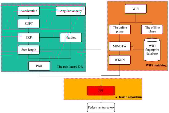
Figure 1. The structure of the indoor navigation algorithm.

3.1. The Gait-Based PDR

3.1.1. EKF

In the PDR module, EKF is a very important technology, which mainly uses the characteristic of ZUPT to reduce cumulative error. When zero velocity is detected, ZUPT is triggered. The EKF works to eliminate noise. The EKF system equation reads

$$\begin{array}{ccc}\hfill \delta {\mathit{X}}_k& =& {\mathit{F}}_{k-1}\delta {\mathit{X}}_{k-1}+{\mathit{\omega }}_{k-1}\hfill \end{array}$$

(1)

$$\begin{array}{ccc}\hfill \delta {\mathit{Z}}_k& =& {\mathit{H}}_k\delta {\mathit{X}}_k+{\mathit{\nu }}_k\hfill \end{array}$$

(2)

where $\delta {\mathit{X}}_k={\left[r_z,v_z,S_{roll},S_{pitch},S_{yaw},{\epsilon }_{v_z},{\epsilon }_{roll},{\epsilon }_{pitch},{\epsilon }_{yaw}\right]}_k^T$ is a 9-element state vector at the k-th epoch; $r_z$ and $v_z$ represent the vertical displacement and vertical velocity, respectively. $S_{roll}$, $S_{pitch}$, and $S_{yaw}$ represent the attitude angles; ${\epsilon }_{v_z}$ represents the bias of the vertical velocity; ${\epsilon }_{roll}$, ${\epsilon }_{pitch}$, and ${\epsilon }_{yaw}$ represent the biases of the attitude angle; ${\mathit{F}}_{k-1}$ represents the state transition matrix; ${\mathit{H}}_k$ represents the observation matrix; ${\mathit{\omega }}_{k-1}$ and ${\mathit{\nu }}_k$ represent the state transition noise and the observation noise, respectively.

3.1.2. Step Length

When walking, the vertical displacement of the user has an approximate periodicity. Step length is estimated by using the periodic characteristics. The vertical displacement is obtained by double integral vertical acceleration.

$$S_{VD}={\int }_{t1}^{t2}{\int }_{t1}^{t2}{a}_z\left(t\right)dtdt$$

(3)

where $t1$ and $t2$ represent the beginning and ending times, respectively; and $S_{VD}$ represents the vertical displacement. According to the inverted pendulum model, the pedestrian step length is calculated as follows

$$D_{SL}=2\sqrt{L^2-{(L-S_{VD})}^2}$$

(4)

where $D_{SL}$ represents the step length; L represents the distance between the smartphone and the ground.

3.1.3. Heading

Quaternion vectors are updated by gyroscope readings. The direction cosine matrix is then updated by the quaternion vector. The attitude angle based on the directional cosine matrix is obtained. When the gyroscope acquires the triaxial angular velocity, the triaxial angular increment is calculated. The quaternion vector ($q_{k+1}=\left[q_1,q_2,q_3,q_4\right]$) at the $(k+1)-th$ epoch is $q_{k+1}=\left[Icos\frac{\Delta {\theta }_k}{2}+\Delta \Theta \frac{sin\frac{\Delta {\theta }_k}{2}}{\Delta {\theta }_k}\right]q_k$, where I represents a 3 identity matrix; $\Delta {\theta }_k$ represents the angle increment; $\Delta \Theta$ represents skew symmetric matrix of angular increments. The direction cosine matrix calculated based on the quaternion vector is $C_b^n=\left[\begin{array}{ccc}{q}_1^2-q_2^2-q_3^2+q_4^2& 2q_1{q}_2-2q_3{q}_4& 2q_1{q}_3+2q_2{q}_4\\ 2q_1{q}_2+2q_3{q}_4& -q_1^2+q_2^2-q_3^2+q_4^2& 2q_2{q}_3-2q_1{q}_4\\ 2q_1{q}_3-2q_2{q}_4& 2q_2{q}_3+2q_1{q}_4& -q_1^2-q_2^2+q_3^2+q_4^2\end{array}\right]$. The attitude angle $[\vartheta ,\varphi ,\phi ]$ based on the direction cosine matrix is $\vartheta ={tan}^{-1}\frac{-C_b^n(3,1)}{\sqrt{{\left(C_b^n(3,2)\right)}^2+{\left(C_b^n(3,3)\right)}^2}}$, $\varphi ={tan}^{-1}\frac{C_b^n(3,2)}{C_b^n(3,3)}$, $\phi ={tan}^{-1}\frac{C_b^n(2,1)}{C_b^n(1,1)}$, where $\vartheta$, $\varphi$ and $\phi$ are called pitch, roll and yaw, respectively.

3.1.4. PDR

With direction, step length, and position at the previous epoch, PDR estimates the user’s position.

$$\left[\begin{array}{c}{x}_{k+1}\\ y_{k+1}\end{array}\right]=\left[\begin{array}{c}{x}_k\\ y_k\end{array}\right]+D_{SL}\left[\begin{array}{c}cos\phi \\ sin\phi \end{array}\right]$$

(5)

where $\left[\begin{array}{c}{x}_k\\ y_k\end{array}\right]$ denotes the pedestrian position at the k epoch; $D_{SL}$ and $\phi$ denote the pedestrian step length and heading.

3.2. WiFi Fingerprint Matching

The fingerprint database <location, RSS> is constructed during the offline phase. To reduce the time and labor costs, the walk-survey approach combining the landmarks and a constant-speed assumption is used [23]. During the offline phase, firstly, the spatial location of the navigation area is measured, and then the fingerprint is collected. The spatial position and the corresponding fingerprint are stored in the database. The following is the WiFi fingerprint of the $j-th$ reference point.

$${FW}_i=\left\{{pos}_i,\left({mac}_{i,1},{RSS}_{i,1}\right),\left({mac}_{i,2},{RSS}_{i,2}\right),\left({mac}_{i,j},{RSS}_{i,j}\right),\cdots ,\left({mac}_{i,m},{RSS}_{i,m}\right)\right\}$$

(6)

where ${pos}_i$ represnets the $i-th$ reference points’s cooordinate; ${mac}_{i,j}$ and ${RSS}_{i,j}$ represent the media access control address and $RSS$ of the $j-th$ AP at the $i-th$ reference point, respectively; and m represents the number of available APs at the $i-th$ reference point.

During the online phase, the WiFi fingerprint is matched with the fingerprints in the reference database. The position corresponding to the most similar fingerprint is usually taken as the location of pedestrians. There are a variety of matching methods [18]. WiFi fingerprint matching algorithm uses multi-dimensional dynamic time warping algorithm, as shown in the Algorithm 1.

Algorithm 1 Multi-dimensional dynamic time warping for WiFi fingerprint matching

Input: The WiFi signal $\mathbf{R}$ with length n during the online phase and the WiFi fingerprint signal ${\mathbf{R}}_{\mathbf{db}}$ with length m during the offline phase. for i = 1 to n do    for j = 1 to m do        $\mathbf{d}(i,j)={\sum }_{k=1}^K{\displaystyle (}\mathbf{R}(k,i)-{\mathbf{R}}_{\mathbf{db}}{(k,j)}^2{\displaystyle )}$.    End End $\mathbf{D}(1,1)=\mathbf{d}(1,1)$. for k = 2 to n do     $\mathbf{D}(k,1)=\mathbf{d}(k,1)+\mathbf{D}(k-1,1)$.     for i = 2 to m do           $\mathbf{D}(1,i)=\mathbf{d}(1,i)+\mathbf{D}(1,i-1)$.           $\mathbf{D}(k,i)=\mathbf{d}(k,i)+min\left(\right[\mathbf{D}(k-1,i),\mathbf{D}(k-1,i-1),\mathbf{D}(k,i-1)\left]\right)$.      End End Output: The WiFi fingerprint distance $\mathbf{D}$.

Based on the weighted average of the k selected reference locations with the minimum Euclidean distance, the WKNN approach is used. The WiFi matching results is calculated as

$$\left[\begin{array}{c}\widehat{x}\\ \widehat{y}\end{array}\right]=\sum _{i=1}^k\frac{c_i}{C}\left[\begin{array}{c}{x}_i\\ y_i\end{array}\right]$$

(7)

where $c_i=1/D_i$, $C={\sum }_{i=1}^k{c}_i$; $\left[\begin{array}{c}{x}_i\\ y_i\end{array}\right]$ represents the position of the $i-th$ selected reference point; $\left[\begin{array}{c}\widehat{x}\\ \widehat{y}\end{array}\right]$ represents the estimated position.

3.3. FPF

The Federated Kalman filter is an effective filtering technique in linear systems affected by Gaussian noise. In nonlinear systems affected by Gaussian noise, an EKF or an unscented Kalman filter is used to obtain global state estimates. However, errors are introduced in the linearization process, which leads to filter divergence in the worst case. Therefore, it is necessary to apply FPF to nonlinear non-Gaussian systems.

In FPF, the reference system is directly output to the main filter on the one hand, and output to each sub-filter as a measurement value on the other hand. The output of each subsystem is only given to the corresponding sub-filter. Each sub-filter obtains a local estimate ${\widehat{\mathbf{X}}}_i$ and its covariance matrix ${\mathbf{P}}_i$ through particle filtering according to the state equation and measurement equation, and then sends it to the main filter and the estimated value of the main filter for fusion to obtain the global optimal estimate. In addition, after each filtering stage is completed, the global filter feeds back the results ${\mathbf{X}}_g$, ${\mathbf{P}}_g$ to each sub-filter and the main filter according to the principle of information conservation. It can be seen from the algorithm principle and process of PF that the PF filtering process obtains the posterior distribution of the state quantity, thereby obtaining the mean and variance information of the state quantity. The algorithm implementation process of FPF is as follows

Step 1 

Initialize particles and their corresponding weights.

Step 2 

Information distribution process. FPF distributes the combined system initial value information to each local filter.

$$\begin{array}{ccc}\hfill {\widehat{\mathbf{X}}}_i& =& {\widehat{\mathbf{X}}}_g\hfill \end{array}$$

(8)

$$\begin{array}{ccc}\hfill {\mathbf{P}}_i& =& {\beta }_i^{-1}{\mathbf{P}}_g\hfill \end{array}$$

(9)

$$\begin{array}{ccc}\hfill {\mathbf{P}}_m& =& {\beta }_m^{-1}{\mathbf{P}}_g\hfill \end{array}$$

(10)

$$\begin{array}{ccc}\hfill {\mathbf{Q}}_i& =& {\beta }_i^{-1}{\mathbf{Q}}_g\hfill \end{array}$$

(11)

$$\begin{array}{ccc}\hfill {\mathbf{Q}}_m& =& {\beta }_m^{-1}{\mathbf{Q}}_g\hfill \end{array}$$

(12)

where ${\beta }_i$ and ${\beta }_m$ represent the sub-filter information distribution coefficient and the main filter distribution coefficient, respectively, and satisfies ${\sum }_{i=1}^N{\beta }_i+{\beta }_m=1$; ${\mathbf{P}}_i$ and ${\mathbf{P}}_m$ represent the estimated sub-filter covariance and the estimated main filter covariance, respectively, and satisfies ${\sum }_{i=1}^N{\mathbf{P}}_i^{-1}+{\mathbf{P}}_m^{-1}={\mathbf{P}}_g^{-1}$; ${\mathbf{Q}}_i$ and ${\mathbf{Q}}_m$ repesent the sub-filter system noise covariance and the main system noise covariance, respectively, and satisfies ${\sum }_{i=1}^N{\mathbf{Q}}_i^{-1}+{\mathbf{Q}}_m^{-1}={\mathbf{Q}}_g^{-1}$.

Step 3 

Each sub-filter filters based on its own equation of state. When $k\ge 1$,

• Extract N samples $\left\{x_k^i,i=1,2,...,N\right\}$ from the importance density function $q\left(x_k^i\right|x_{k-1}^i)=N(x_k^i;{\widehat{x}}_k^i,P_k^i)$.
• Calculate the weight of each particle ${\omega }_i={\omega }_{k-1}^{i}p\left(z_k\right|x_k^i)$
• Normalized particle weights ${\tilde{\omega }}_k^i=\frac{{\omega }_k^i}{{\sum }_{i=1}^N{\omega }_k^i}$
• Resample particles to get a new set of samples $\{x_k^i\sim N(x_k^i;{\widehat{x}}_k^i,P_k^i),i=1,2,\cdots ,N\}$
• Make a status update. The state and variance information is calculated according to the particles and their corresponding weights ${\widehat{x}}_k={\sum }_{i=1}^N{\widehat{\omega }}_k^i{x}_k^i$ and $P_k={\sum }_{i=1}^N{\widehat{\omega }}_k^i({\widehat{x}}_k-x_k^i){({\widehat{x}}_k-x_k^i)}^T$.

Step 4 

Perform global information fusion. After obtaining the local estimation of each sub-filter and the estimation of the main filter, the global state filter value and variance estimation value are obtained ${\widehat{\mathbf{x}}}_g\left(k\right)={\mathbf{P}}_g\left(k\right){\sum }_{i=1}^N\left({\mathbf{P}}_i^{-1}\left(k\right){\widehat{\mathbf{x}}}_i\left(k\right)\right)$ and ${\mathbf{P}}_g\left(k\right)={\left({\sum }_{i=1}^N{\mathbf{P}}_i^{-1}\left(k\right)\right)}^{-1}$.

Step 5 

After obtaining the global state and variance estimation information, the local filters are allocated and reset according to the information allocation principle based on the formula in Step 2.

Step 6 

Let $k=k+1$, go back to Step 3 and repeat the above steps.

3.4. PDR/WiFi-Based FPF Integrated Navigation System Model

Based on the Monte Carlo method, particle filter (PF) uses a particle set to represent probability, which is used in any form of the state-space model. The core idea is to express its distribution by extracting random state particles from a posteriori probability. The state equation is expressed as follows [24]

$${\mathbf{X}}_k=f({\mathbf{X}}_{k-1},{\mathbf{W}}_{k-1})$$

(13)

where ${\mathbf{X}}_k$ represents the state at the k-th epoch; ${\mathbf{W}}_{k-1}$ is the process noise of the system. When the system noise conforms to zero mean and Q variance, the Gaussian distribution is expressed as

$${\mathbf{W}}_{k-1}\sim N(0,Q)$$

(14)

It is assumed that the noise with heading change obeys the Gaussian distribution of zero mean. Combined with PDR, the state equation is written as [25]

$$\begin{array}{cc}\hfill {\mathbf{X}}_k& =\left[\begin{array}{c}{H}_k\\ x_k\\ y_k\end{array}\right]=\left[\begin{array}{c}{H}_{k-1}\\ x_{k-1}\\ y_{k-1}\end{array}\right]+\left[\begin{array}{c}\Delta H\\ S{L}_{k}cos\left({\mathrm{H}}_k\right)\\ S{L}_{k}sin\left(H_k\right)\end{array}\right]+\left[\begin{array}{c}{W}_{H,k-1}\\ W_{x,k-1}\\ W_{y,k-1}\end{array}\right]\hfill \end{array}$$

(15)

where $H_k$ represents the pedestrian heading at the k-th epoch, respectively; ${[x_k,y_k]}^T$ represents the pedestrian position at the k-th epoch; $△H$ represents the change of heading; ${\left[W_{H,k-1},W_{x,k-1},W_{y,k-1}\right]}^T$ represents the Gaussian noise of heading and pedestrian position, respectively.

It is a common technique to use fingerprints for indoor navigation [26,27]. The sequential fingerprint matching algorithm is introduced in reference [18]. Combined with the WiFi positioning results and step length, the observation equations are written as follows

$$\begin{array}{ccc}\hfill {\mathbf{Z}}_{1,k}& =& D_{SL}+v_{SL}\hfill \end{array}$$

(16)

$$\begin{array}{ccc}\hfill {\mathbf{Z}}_{2,k}& =& \left[\begin{array}{c}{x}_{wifi}\hfill \\ y_{wifi}\hfill \end{array}\right]+\left[\begin{array}{c}{v}_x\hfill \\ v_y\hfill \end{array}\right]\hfill \end{array}$$

(17)

where $v_{SL}$ represents the step length noise with zero mean and $R_1$ variance; ${[x_{wifi},y_{wifi}]}^T$ represents the WiFi matching results; ${[{\upsilon }_x,{\upsilon }_y]}^T$ represents the corresponding observation noise with zero mean and $R_2$ variance.

After the production of new particles, the posterior distribution of system state is written as [24]

$$p\left({\mathbf{X}}_{0:k}\mid {\mathbf{Z}}_{1:k}\right)\propto p\left({\mathbf{X}}_{0:k-1}\mid {\mathbf{Z}}_{1:k-1}\right)p\left({\mathbf{Z}}_k\mid {\mathbf{X}}_k\right)p\left({\mathbf{X}}_k\mid {\mathbf{X}}_{k-1}\right)$$

(18)

It is difficult to solve the analytical solution of the posterior distribution. Instead of solving the analytical solution, the approximate solution has been well developed. A large number of particles are used to approximate a posteriori distribution. To deal with the problem of a posteriori distribution in sampling, a resampling technique is proposed. Importance distribution is defined as

$$q\left({\mathbf{X}}_{0:k}\mid {\mathbf{Z}}_{1:k}\right)=q\left({\mathbf{X}}_{0:k-1}\mid {\mathbf{Z}}_{1:k-1}\right)q\left({\mathbf{X}}_k\mid {\mathbf{X}}_{0:k-1},{\mathbf{Z}}_{1:k}\right)$$

(19)

The recursive importance weight of each generation of particles is calculated as [24]

$${\omega }_k^i\propto {\omega }_{k-1}^i\frac{p\left({\mathbf{Z}}_k\mid {\mathbf{X}}_k^i\right)p\left({\mathbf{X}}_k^i\mid {\mathbf{X}}_{k-1}^i\right)}{q\left({\mathbf{X}}_k^i\mid {\mathbf{X}}_{0:k-1}^i,{\mathbf{Z}}_{1:k}\right)}$$

(20)

The effective particle weights are updated as

$$\begin{array}{cc}\hfill {\omega }_k^i& =\frac{p\left({\mathbf{X}}_{0:k}^i\mid {\mathbf{Z}}_{1:k}\right)}{q\left({\mathbf{X}}_{0:k}^i\mid {\mathbf{Z}}_{1:k}\right)}\hfill \\ \hfill & =\frac{1}{{\left(2\pi \right)}^{m/2}{\left|\mathbf{R}\right|}^{\frac{1}{2}}}{e}^{-{\left[{\mathbf{Z}}^{*}-h\left({\widehat{\mathbf{X}}}_k\right)\right]}^T{\mathbf{R}}^{-1}\left[{\mathbf{Z}}^{*}-h\left({\widehat{\mathbf{X}}}_k\right)\right]}\hfill \end{array}$$

(21)

where m represents the dimension of the observation equation; ${\mathbf{Z}}^{*}={\mathbf{Z}}_1$ or ${\mathbf{Z}}_2$ and $h\left({\widehat{\mathbf{X}}}_k\right)$ represent observations and estimated observations, respectively; $\mathbf{R}$ represents the Gaussian noise of the observation equation.

Normalize the particle weights as follows

$${\tilde{\omega }}_k^i=\frac{{\omega }_k^i}{{\sum }_{i=1}^N{\omega }_k^i}$$

(22)

After obtaining each subfilter estimate, the value of the global state filter is

$$\begin{array}{ccc}\hfill {\widehat{\mathbf{X}}}_g\left(k\right)& =& {\mathbf{P}}_g\left(k\right)\sum _{i=1}^N\left({\mathbf{P}}_i^{-1}\left(k\right){\widehat{\mathbf{X}}}_i\left(k\right)\right)\hfill \end{array}$$

(23)

$$\begin{array}{ccc}\hfill {\mathbf{P}}_g\left(k\right)& =& {\left(\sum _{i=1}^N{\mathbf{P}}_i^{-1}\left(k\right)\right)}^{-1}\hfill \end{array}$$

(24)

4. Experimental Results

4.1. Experimental Preparation

As shown in Figure 2, two typical indoor navigation scenarios are selected to be tested. According to the recommendations of the international standard ISO/IEC 18305 [28], the real reference points on the ground need sufficient density and these points are random. We set the distance between the two adjacent reference points to 3 to 10 m. The real reference points on the ground are measured by a laser rangefinder. A smartphone Honor 50 is used to construct a WiFi fingerprint database in the offline phase. A smartphones Nexus 5X is used to collect acceleration, angular velocity, and WiFi in the online phase. Smartphone modes include calling, dangling, handheld, and pocketed. In the offline phase, the surveyor collects WiFi signals to build a reference fingerprint database. In the online phase, the measured WiFi is used to match with the reference fingerprint. The corresponding position of the most similar fingerprint is taken as the fingerprint matching result. Table 1 shows the process noise covariance Q, the step length measurement noise covariance $R_1$, and the position measurement noise covariance $R_2$.

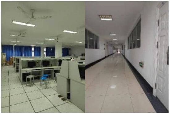
Figure 2. Experimental scenarios.

Table 1. Parameters setting.

Parameters	Q	${\mathit{R}}_{\mathbf{1}}$	${\mathit{R}}_{\mathbf{2}}$
Values	$\left[\begin{array}{ccc}0.1& 0& 0\\ 0& 0.1& 0\\ 0& 0& 0.1\end{array}\right]$	1	$\left[\begin{array}{cc}1& 0\\ 0& 1\end{array}\right]$

4.2. WiFi Distribution

Figure 3 shows the WiFi distribution in the test scenario. The red line on the xy plane represents the true trajectory of the pedestrian. The value of the z-axis represents the number of APs. As can be seen from the figure, the number of WiFi APs is abundant enough to be used for fingerprint matching.

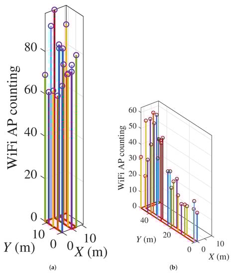
Figure 3. WiFi distribution. (a) An Laboratory. (b) An Office Building.

4.3. Walking Experiment in an Laboratory

An adult male holding a smartphone walks in a predefined indoor area at a normal walking speed. Figure 4, Figure 5, Figure 6, Figure 7 and Figure 8 show the navigation trajectories, position errors and cumulative distribution functions (CDFs) for PDR, WiFi, and FPF. Table 2 shows the Average Error (AE), Root Mean Square Error (RMSE), Maximum Error (ME), and Circular Error Probability (CEP), respectively. Compared to PDR and WiFi, FPF reduces errors by as follows: (a) for AE: 87.74% and 19.57%, respectively; (b) for RMSE: 87.36% and 23.81%, respectively; (c) for ME: 86.98% and 36.53%; (d) CEP of 75%: 86.08% and 18.97%; and (e) for CEP of 95%: 87.05% and 35.96%. The longer the walking time, the greater the deviation of PDR is. There is mismatching in WiFi fingerprint matching, which is mainly due to the multi-channel effect and reflection effect. Based on the information sharing mechanism, FPF effectively integrates PDR and WiFi, reducing position errors.

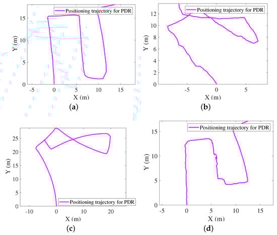
Figure 4. Navigation trajectories for PDR. (a) Calling mode. (b) Dangling mode. (c) Handheld mode. (d) pocketed mode.

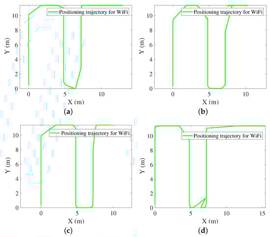
Figure 5. Navigation trajectories for WiFi. (a) Calling mode. (b) Dangling mode. (c) Handheld mode. (d) Pocketed mode.

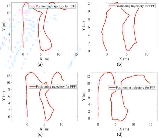
Figure 6. Navigation trajectories for FPF. (a) Calling mode. (b) Dangling mode. (c) Handheld mode. (d) pocketed mode.

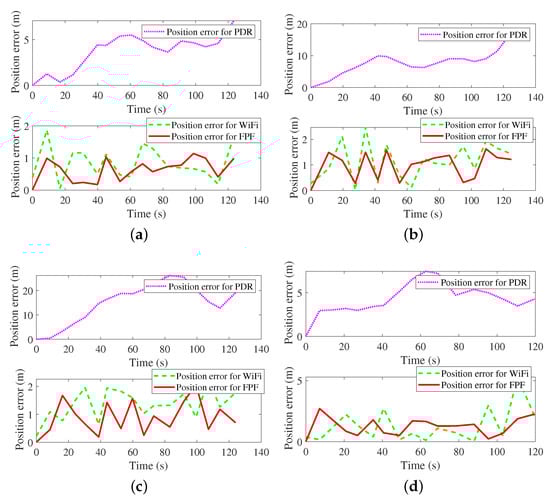
Figure 7. Position errors with different modes. (a) Position errors with calling mode. (b) Position errors with dangling mode. (c) Position errors with handheld mode. (d) Position errors with pocketed mode.

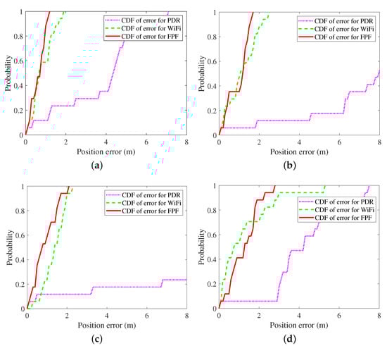
Figure 8. CDFs of errors with different modes. (a) CDFs of errors with calling mode. (b) CDFs of errors with dangling mode. (c) CDFs of errors with handheld mode. (d) CDFs of errors with pocketed mode.

Table 2. Position errors for PDR, WiFi and FPF (m).

Motion Modes	Algorithms	AE	RMSE	ME	CEP of 75%	CEP of 95%
Calling mode	PDR	3.7	4.17	7.05	4.88	7.02
	WiFi	0.85	0.99	1.87	1.19	1.82
	FPF	0.63	0.71	1.14	0.93	1.12
Dangling mode	PDR	7.76	8.58	17.25	9.09	17.22
	WiFi	1.14	1.35	2.47	1.74	2.42
	FPF	0.97	1.1	1.63	1.38	1.62
Handheld mode	PDR	14.78	16.81	26.19	20.44	26.12
	WiFi	1.36	1.46	2.26	1.79	2.22
	FPF	0.89	1.06	2.06	1.44	2.02
Pocketed mode	PDR	4.26	4.61	7.42	5.18	7.42
	WiFi	1.3	1.87	5.28	2.08	5.22
	FPF	1.25	1.45	2.71	1.76	2.72
General	PDR	7.63	8.54	14.48	9.9	14.45
	WiFi	1.16	1.42	2.97	1.7	2.92
	FPF	0.94	1.08	1.89	1.38	1.87

Walking Experiment in an Office Building

PF used WiFi results as the observation equation. Hu proposed an adaptive particle filter (APF) to estimate indoor pedestrian locations [29]. APF used the difference between PDR and WiFi results as the observation equation. Figure 9, Figure 10, Figure 11, Figure 12, Figure 13 and Figure 14 show the navigation trajectories, position errors and CDFs for PDR, PF, APF, and FPF. Table 3 shows AE, RMSE, ME, and CEP, respectively. Compared to PDR, PF and APF, FPF reduces errors by as follows: (a) for AE: 93.99%, 20.21%, and 56.71%, reespctively; (b) for RMSE: 93.7%, 18.91%, and 58.62%, respectively; (c) for ME: 93.92%, 13.09%, and 66.08%, respectively; (d) for CEP of 75%: 93.59%, 22.01%, and 51.79%, respectively; and (e) for CEP of 95%: 93.05%, 17.67%, and 60.59%, respectively. After introducing the step length observation equation, FPF effectively improves the pedestrian location estimation.

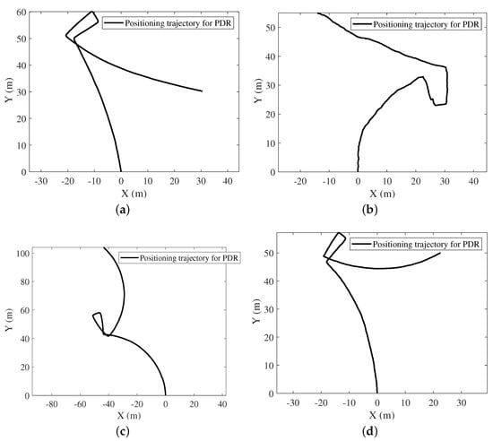
Figure 9. Navigation trajectories for PDR. (a) Calling mode. (b) Dangling mode. (c) Handheld mode. (d) pocketed mode.

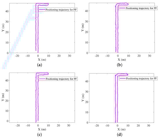
Figure 10. Navigation trajectories for PF. (a) Calling mode. (b) Dangling mode. (c) Handheld mode. (d) pocketed mode.

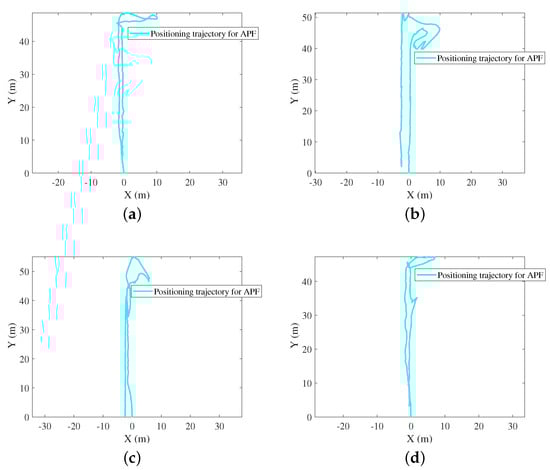
Figure 11. Navigation trajectories for APF. (a) Calling mode. (b) Dangling mode. (c) Handheld mode. (d) Pocketed mode.

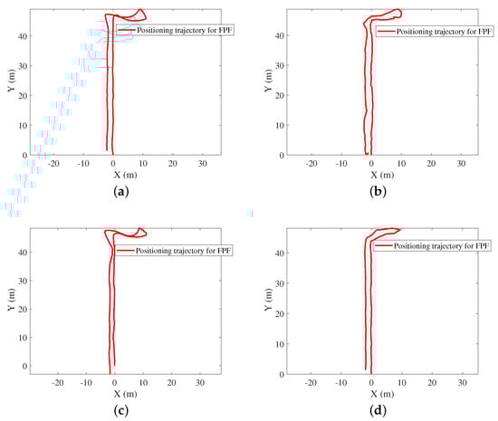
Figure 12. Navigation trajectories for FPF. (a) Calling mode. (b) Dangling mode. (c) Handheld mode. (d) pocketed mode.

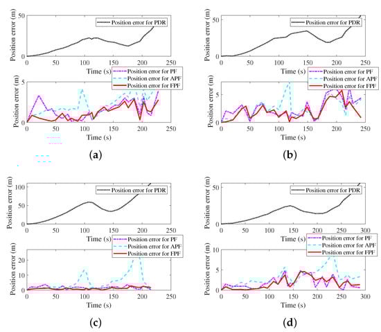
Figure 13. Position errors with different modes. (a) Position errors with calling mode. (b) Position errors with dangling mode. (c) Position errors with handheld mode. (d) Position errors with pocketed mode.

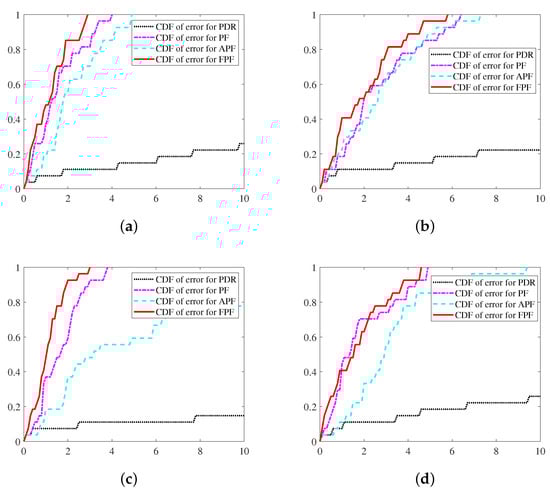
Figure 14. CDFs of errors with different modes. (a) CDFs of errors with calling mode. (b) CDFs of errors with dangling mode. (c) CDFs of errors with handheld mode. (d) CDFs of errors with pocketed mode.

Table 3. Position errors for PDR, PF, APF, and FPF (m).

Motion Modes	Algorithms	AE	RMSE	ME	CEP of 75%	CEP of 95%
Calling mode	PDR	16.26	18.89	43.36	22.31	32.07
	PF	1.49	1.82	3.8	2.13	3.37
	APF	2.18	2.54	4.86	3.13	4.83
	FPF	1.18	1.45	2.84	1.86	2.77
Dangling mode	PDR	22.67	26.48	55.95	32.13	42.67
	PF	2.57	3.13	6.2	3.73	5.87
	APF	2.64	3.23	7.04	4.03	6.27
	FPF	2.01	2.53	5.73	2.93	4.67
Handheld mode	PDR	42.62	50.82	110.29	57.93	91.27
	PF	1.66	1.92	3.73	2.23	3.47
	APF	5.9	8.55	26.32	7.23	18.67
	FPF	1.12	1.32	2.96	1.53	2.47
Pocketed mode	PDR	18.3	22.3	55.77	24.13	41.87
	PF	1.8	2.33	4.83	3.13	4.83
	APF	3.14	3.71	9.34	3.76	6.87
	FPF	1.69	2.16	4.6	2.43	4.53
General	PDR	24.96	29.62	66.34	34.13	51.97
	PF	1.88	2.3	4.64	2.81	4.39
	APF	3.47	4.51	11.89	4.54	9.16
	FPF	1.5	1.87	4.03	2.19	3.61

5. Conclusions

Aiming at the cumulative error of PDR and the mismatching of WiFi fingerprints, this paper takes the step length and WiFi matching results as observation equations, and proposes FPF. The experimental results show that the average positioning accuracy of FPF is 0.94 m and 1.5 m. One of the advantages of this algorithm is that it does not need to deploy additional infrastructure and provides a low-cost and high-precision indoor navigation and positioning scheme.

However, when the positioning area is large, the construction and maintenance of the WiFi fingerprint database take time and effort. How to reduce the burden of building and maintaining a fingerprint database is a topic worthy of further research. PF has a large amount of calculation, which has certain requirements for the hardware of the smartphone. How to reduce the computational complexity of PF is another topic worth studying. The algorithm proposed in this paper needs to be tested in more experimental scenarios.

References

- Xu, Y.; Cao, J.; Shmaliy, Y.S.; Zhuang, Y. Distributed Kalman filter for UWB/INS integrated pedestrian localization under colored measurement noise. Satell. Navig. 2021, 2, 22. [Google Scholar] [CrossRef]
- El-Sheimy, N.; Li, Y. Indoor navigation: State of the art and future trends. Satell. Navig. 2021, 2, 7. [Google Scholar] [CrossRef]
- Zheng, L.; Wu, Z.; Zhou, W.; Weng, S.; Zheng, H. A smartphone based hand-held indoor positioning system. In Frontier Computing; Hung, J.C., Yen, N.Y., Li, K.-C., Eds.; Springer: Singapore, 2016; pp. 639–650. [Google Scholar]
- Li, Y.; Zhuang, Y.; Lan, H.; Zhang, P.; Niu, X.; El-Sheimy, N. Self-contained indoor pedestrian navigation using smartphone sensors and magnetic features. IEEE Sens. J. 2016, 16, 7173–7182. [Google Scholar] [CrossRef]
- Chen, J.; Ou, G.; Peng, A.; Zheng, L.; Shi, J. An INS/floor-plan indoor localization system using the firefly particle filter. ISPRS Int. J. Geo-Inf. 2018, 7, 324. [Google Scholar] [CrossRef]
- Kang, W.; Han, Y. SmartPDR: Smartphone-based pedestrian dead reckoning for indoor localization. IEEE Sens. J. 2014, 15, 2906–2916. [Google Scholar] [CrossRef]
- Bargshady, N.; Garza, G.; Pahlavan, K. Precise Tracking of Things via Hybrid 3-D Fingerprint Database and Kernel Method Particle Filter. IEEE Sens. J. 2016, 16, 8963–8971. [Google Scholar] [CrossRef]
- Wang, G.; Chen, H.; Li, Y.; Jin, M. On received-signal-strength based localization with unknown transmit power and path loss exponent. IEEE Wirel. Commun. Lett. 2012, 16, 536–539. [Google Scholar] [CrossRef]
- Huang, Q.; Zhang, Y.; Ge, Z.; Lu, C. Refining Wi-Fi based indoor localization with Li-Fi assisted model calibration in smart buildings. In Proceedings of the 2016 International Conference on Computing in Civil and Building Engineering, Osaka, Japan, 6–8 July 2016; pp. 1–8. [Google Scholar]
- Yu, C.; Lan, H.; Liu, Z.; El-Sheimy, N.; Yu, F. Indoor Map Aiding/map Matching Smartphone Navigation Using Auxiliary Particle Filter. In Proceedings of the 2016 China Satellite Navigation Conference (CSNC); Springer: Singapore, 2016. [Google Scholar]
- Chen, J.; Song, S.; Gong, Y.; Zhang, S. An indoor fusion navigation algorithm using HV-derivative dynamic time warping and the chicken particle filter. In Proceedings of the China Satellite Navigation Conference (CSNC), Changsha, China, 18–20 May 2016. [Google Scholar]
- Foxlin, E. Pedestrian Tracking with Shoe-mounted Inertial Sensors. IEEE Comput. Graph. 2005, 25, 38–46. [Google Scholar] [CrossRef]
- Elwell, J. Inertial Navigation for the Urban Warrior. In Proceedings of the Digitization of the Battlespace IV, Orlando, FL, USA, 9 July 1999. [Google Scholar]
- Jiménez, A.R.; Seco, F.; Prieto, J.C.; Guevara, J. Indoor Pedestrian Navigation Using an INS/EKF Framework for Yaw Drift Reduction and a Foot-mounted IMU. In Proceedings of the 2010 7th Workshop on Positioning, Navigation and Communication, Dresden, Germany, 11–12 March 2010; IEEE: Piscataway, NJ, USA, 2010; pp. 135–143. [Google Scholar]
- Borenstein, J.; Ojeda, L. Heuristic Drift Elimination for Personnel Tracking Systems. J. Navig. 2010, 63, 591. [Google Scholar] [CrossRef]
- Bahl, P.; Padmanabhan, V.N. RADAR: An in-building RF-based user location and tracking system. In Proceedings of the IEEE INFOCOM 2000 Conference on Computer Communications, Tel Aviv, Israel, 26–30 March 2000; IEEE: Piscataway, NJ, USA, 2000. [Google Scholar]
- Chen, J.; Ou, G.; Peng, A.; Zheng, L.; Shi, J. An INS/WiFi indoor localization system based on the Weighted Least Squares. IEEE Sens. 2005, 18, 1458. [Google Scholar] [CrossRef]
- Li, Y.; Zhuang, Y.; Lan, H.; Niu, X.; El-Sheimy, N. A profile-matching method for wireless positioning. IEEE Commun. Lett. 2016, 20, 2514–2517. [Google Scholar] [CrossRef]
- Cao, X.; Zhuang, Y.; Yang, X.; Sun, X.; Wang, X. A universal Wi-Fi fingerprint localization method based on machine learning and sample differences. Satell. Navig. 2021, 2, 27. [Google Scholar] [CrossRef]
- Li, Z.; Liu, C.; Gao, J.; Li, X. An improved WiFi/PDR integrated system using an adaptive and robust filter for indoor localization. ISPRS Int. J. Geo-Inf. 2016, 5, 224. [Google Scholar] [CrossRef]
- Sun, M.; Wang, Y.; Xu, S.; Cao, H.; Si, M. Indoor Positioning Integrating PDR/Geomagnetic Positioning Based on the Genetic-Particle Filter. Appl. Sci. 2020, 10, 668. [Google Scholar] [CrossRef]
- Wang, Z.; Yang, Z.; Wang, Z. An Adaptive Indoor Positioning Method Using Multisource Information Fusion Combing Wi-Fi/MM/PDR. IEEE Sens. J. 2022, 22, 6010–6018. [Google Scholar] [CrossRef]
- Li, Y.; Zhuang, Y.; Lan, H.; Zhang, P.; Niu, X.; El-Sheimy, N. WiFi-aided magnetic matching for indoor navigation with consumer portable devices. Micromachines 2015, 6, 747–764. [Google Scholar] [CrossRef]
- Yin, S.; Zhu, X. Intelligent Particle Filter and Its Application to Fault Detection of Nonlinear System. IEEE Trans. Ind. Electron. 2015, 62, 3852–3861. [Google Scholar] [CrossRef]
- Xie, H.; Gu, T.; Tao, X.; Ye, H.; Lu, J. A Reliability-augmented Particle Filter for Magnetic Fingerprinting Based Indoor Localization on Smartphone. IEEE Trans. Mob. Comput. 2015, 14, 1877–1892. [Google Scholar] [CrossRef]
- Fang, S.H.; Lin, T.N. A Dynamic System Approach for Radio Location Fingerprinting in Wireless Local Area Networks. IEEE Trans. Commun. 2010, 58, 1020–1025. [Google Scholar] [CrossRef]
- Khalajmehrabadi, A.; Gatsis, N.; Akopian, D. Modern WLAN Fingerprinting Indoor Positioning Methods and Deployment Challenges. IEEE Comput. Surv. Tutor. 2017, 19, 1974–2002. [Google Scholar] [CrossRef]
- ISO/IEC 18305. Information Technology—Real Time Locating Systems—Test and Evaluation of Localization and Tracking Systems. 2016. Available online: https://www.iso.org/standard/62090.html (accessed on 16 October 2022).
- Hu, Y.; Peng, A.; Tang, B.; Xu, H. An Indoor Navigation Algorithm Using Multi-Dimensional Euclidean Distance and an Adaptive Particle Filter. Sensors 2021, 21, 8228. [Google Scholar] [CrossRef] [PubMed]
Publisher’s Note: MDPI stays neutral with regard to jurisdictional claims in published maps and institutional affiliations. |
© 2022 by the authors. Licensee MDPI, Basel, Switzerland. This article is an open access article distributed under the terms and conditions of the Creative Commons Attribution (CC BY) license (https://creativecommons.org/licenses/by/4.0/).