1. Introduction
Unmanned aerial vehicles (UAVs) are nowadays used in a wide range of industries, such as healthcare, humanitarian aid or commercial purposes. However, drones can pose a threat to critical infrastructure at the same time, due to their availability and ability to carry various types of weapons (explosives, jammers, etc.). Therefore, their neutralization is currently a highly discussed topic. The drones themselves can be divided into civilian and military, and both groups pose a real threat. They vary only in usage and capability of weapons systems. There are several ways of jamming drones in order to neutralize them. They depend mainly on the type of the communication signal modulation that the drones use and the related band in which the drones operate. This article addresses the issue of civilian UAVs, which are easily accessible and easily customizable. Additionally, there is a problem with their localization due to their small RCS (radar cross-section).
This article focuses on the current overview of UAV neutralization techniques as UAVs are becoming an increasing threat with their growing popularity. Furthermore, this article analyzes the current state-of-the-art machine learning and deep learning methods with a focus on UAV application. Due to the complex UAV control signals and the generally complex signal environment in which UAVs operate, these methods have potential uses to address UAV interference and takeover issues. Various types of research have already been published for UAV neutralization and countermeasures against neutralization [
1,
2,
3,
4,
5,
6]. Due to the popularity of machine learning and deep learning, several studies have also been published about communication signals or wireless networks [
7,
8,
9], which are closely related to the topic of UAVs. Several publications are also focused on applications of these methods to UAV on-board systems, management of the UAV itself or UAV swarms [
9,
10,
11]. Despite all the identified benefits of machine learning in these areas, insufficient research has been conducted on the use of UAV jamming and spoofing.
Table 1 shows recent surveys and reviews focusing on UAV applications, jamming and spoofing techniques, communication signals, or machine and deep learning applications.
As can be seen from
Table 1, a number of studies have been conducted in recent years across the areas of UAV neutralization, communication signals and applications of machine and deep learning methods. However, none of these recent studies connect all of these areas. Therefore, the aim of this study is to provide an overview in the aforementioned areas and link them together. There is potential for the development of more sophisticated UAV neutralization techniques, and the use of deep learning methods for these applications appears to be a promising research topic.
The article is designed as follows. The introductory part is followed by
Section 2, in which basic types of UAV signals and modulations are discussed. Furthermore,
Section 2 also focuses on basic communication protocols used by the most well-known UAV manufacturers.
Section 3 introduces basic techniques of jamming and spoofing. Moreover, practical examples of cyberattacks against UAVs are described here.
Section 4 and
Section 5 focus on the basic description, explanation and division of machine learning and deep learning models. Furthermore, in these sections, practical use of these methods in the researched area is presented. In
Section 6, the simulations of signal modulation classifiers based on various types of neural networks are presented.
Section 7 discusses the advantages and the disadvantages of employing deep learning algorithms in comparison to traditional methods. We also discuss the limitations of previous studies and their comparison. In
Section 8, a conclusion is provided.
2. Signals and Protocols for UAV Communication
In terms of manual control, current commercial drones usually operate in the standard Wi-Fi band (2.4 GHz and 5 GHz). Even basic commercial drones usually have several pre-programmed automatic functions, such as tracking the position of the drone or the “go home” function. The “go home” function guides the drone back to the take-off location according to the GPS (Global Positioning System) if the control signal is lost. The Global Navigation Satellite System (GNSS) is used for these functions. The GPS band in which the drones operate is located at 1574.42 MHz and 1227.60 MHz. Other possible drone remote control bands are at 900 MHz and 1.3 GHz, but these bands are close to the GPS band and may cause interference. At the same time, larger antennas are needed for lower frequencies. This brings another disadvantage in the use of these bands. Nowadays, the integration of the use of 4G and 5G bands for drone control is already beginning [
1,
2,
12]. The basic types of modulations used for communication with drones are discussed below.
2.1. Spread Spectrum Signals
Currently, we have several basic analog modulations (AM, FM, PM—amplitude, frequency and phase modulation) or data modulations (ASK, FSK, PSK—amplitude, frequency and phase shift keying). However, these signals are unsuitable for drone control as they have a fixed carrier signal frequency. Such signals can be easily found and jammed in the spectrum, although some modulations of this type (FSK, PSK) show a certain immunity to interference. However, these signals are easily demodulated, so anyone with sufficient equipment can find out what message is being transmitted. Therefore, spread spectrum signals are used. These types of signals show good resistance to interferences, whether natural (noise) or intentional (jamming). The principle of spectrum spreading consists of modulating a narrowband signal containing information by a pseudorandom broadband signal. By this modulation, the spread spectrum signal is obtained [
1]. In the following paragraphs, various spectrum spreading options are described.
2.1.1. Direct Sequence Spread Spectrum—DSSS
DSSS is the most basic form of spectrum spreading, where a signal with information is modulated by a pseudo-random code (PN code). The resulting signal bandwidth is similar to the PN code bandwidth. The PN code also serves as a demodulation key. DSSS usually uses BPSK or QPSK modulation (binary or quadrature PSK) [
1]. DSSS can theoretically be below the noise level, as for demodulation, it is necessary to know only the PN code, according to which the appropriate signal in the spectrum can be found. Thanks to this, it is difficult for the attacker to find this system in the spectrum at all, let alone effectively jam it. This type of modulation can be disturbed by ultra-wideband (UWB) noise jamming (see
Section 3), but the jamming signal power needs to be 20–40 dB higher than the useful signal power. The described basic principle of DSSS and the block diagram for its implementation are shown in
Figure 1.
2.1.2. Frequency Hopping Spread Spectrum—FHSS
The narrowband information signal is modulated onto a carrier signal with a rapidly changing frequency. The frequency of the carrier signal changes according to the pseudo-random sequence, and the signal remains at one frequency for approximately 5–10 ms. The result of this modulation is a UWB signal. This type of spectrum spreading often uses MSK (minimum shift keying) modulation [
1]. The disadvantage of this type of spectrum spreading is that this signal can be easily found in the spectrum. To prevent transmission, it is usually sufficient to jam about one-third of the frequency jumps. However, due to the unknown sequence of frequency hopping, it is still necessary to jam the entire bandwidth in which the frequency of the carrier signal changes. The block diagram for implementing FHSS is shown in
Figure 2a.
2.1.3. Time Hopping Spread Spectrum—THSS
With THSS, the signal is not transmitted continuously, but is divided into parts and transmitted in individual pulses. Basically, the pulse repetition interval (PRI) and duty cycle are pseudo-randomly changed. In the true sense of the word, THSS is not a type of spectrum spreading. Therefore, it is used in combination with FHSS to create a signal with spread spectrum [
1]. Even though THSS is not exactly a type of spectrum spreading, it can largely increase the resistance to interference, particularly against jamming. For example, THSS is largely used in modern radars, where mainly PRI varies from pulse to pulse or between groups of pulses. There are numerous ways of changing PRI, such as jitter, stagger, etc.
2.1.4. Chirp Spread Spectrum—CSS
Unlike DSSS and FHSS, this type of modulation does not use a pseudo-random code generator to spread the spectrum. Instead, it uses a continuous or discrete change in carrier frequency over time to spread the spectrum. According to various mathematical relations (the simplest is linear dependence—linear frequency modulation), the frequency can increase (upchirp) or decrease (downchirp) [
1]. If the frequency change is not linear, then it is called nonlinear frequency modulation (NLFM). Furthermore, the frequency change may be a combination of upchirp and downchirp (V-shaped LFM—VLFM). The spectrum of such signals uses the entire allocated bandwidth and is resistant to interferences (see
Figure 2b).
2.1.5. Orthogonal Frequency Division Multiplexing—OFDM
OFDM is currently one of the most common modulations that can be found in communication signals in the field of UAVs. It is also the basic modulation used in current modulation schemes such as 802.11 WLAN, 802.16 WiMAX or 3GPP LTE. OFDM, in contrast to conventional modulations, is a digital type of modulation that uses several so-called subcarriers in one channel instead of one carrier. Each of these subcarriers can then be modulated by one of the conventional digital modulations (16 QAM—16 quadrature AM, QPSK, etc.) with a slow symbol rate. The use of several subcarriers results in a comparable data rate with conventional single-carrier modulations in a given band [
13].
Figure 3 shows the principle of generation and demodulation of a signal with OFDM. In the frequency domain, we have many subcarriers that are independently modulated by the required data. These are then converted into OFDM symbols in the time domain using Inverse Fast Fourier Transformation (IFFT). The individual symbols can then be concatenated into one resulting OFDM pulse. A Fast Fourier Transformation (FFT) is then performed at the receiver to obtain the original data. The whole process of the OFDM modulation and demodulation is described in
Figure 4. Firstly, the incoming binary data are baseband modulated by a digital modulation scheme such as BPSK, QPSK, QAM, etc. Secondly, the serial sequence is converted into parallel substreams. Then, the IFFT block converts each substream into an individual subcarrier, thus creating OFDM symbols. In the next block, the guard intervals are appended to the beginning of each OFDM symbol. Lastly, OFDM symbols are converted into a serial sequence of OFDM symbols that modulates high-frequency carriers and is transmitted via a channel. The processes in the receiver are reversed to the described processes in the transmitter [
13,
14,
15].
The function of this type of modulation is based on the concept of orthogonality. This concept is shown in
Figure 5. Each of the subcarriers usually has a spectrum in the form of the sinc(x) function, which results in overlapping spectra between the individual subcarriers. However, if the individual frequencies are orthogonal to each other, the peak of the main lobe of one of the subcarriers corresponds to zeroes for the side lobes of the others. In this case, there is no interference that would prevent a restoration of the original data in the receiver. Consequently, the orthogonality provides high spectral efficiency. Interference between individual subcarriers occurs only in the case of loss of orthogonality [
13,
14].
The term guard interval (GI), mentioned above, refers to cyclic prefix (CP), which is appended to the beginning of every OFDM symbol. Appending of CP reduces the effect of the inter-symbol interference (ISI). ISI occurs due to the transmission in a non-ideal transmission channel. Basically, ISI refers to spreading of the OFDM symbol that results in interference with another symbol. For mitigating ISI, the last N samples of OFDM symbols are copied and appended to the beginning of the OFDM symbol. These last N samples are called the cyclic prefix. The spread OFDM symbol then affects only the CP of the next symbol. This principle is shown in
Figure 6 [
14,
15].
The application of OFDM modulation, which is currently widely used, greatly complicates the detection process of UAVs in the spectrum. Furthermore, it complicates the use of jamming and spoofing techniques, discussed below. Due to these complications, efforts are being made to improve current receivers for successful detection of this type of modulation. One promising way is to use different machine or deep learning techniques (see [
15,
16,
17]). The use of the machine or deep learning methods is explained in
Section 4 and
Section 5.
2.2. Protocols for UAV Communication
There are several protocols that are used for wireless communication between a transmitter (controller) and a receiver (drone). These transmission protocols are characterized by the structure of their data packets, encryption and the type of spectrum spreading (described above) [
1]. Manufacturers usually use one or two types of protocols, so if the appropriate protocol is found, the appropriate drone can be assigned to the particular manufacturer. Jamming techniques that can be used against such drones can then be derived from the knowledge of the protocols.
Table 2 lists well-known vendors and the protocols they use to communicate with UAVs.
2.2.1. MAVLink
MAVLink is an open-source protocol for the transmission of telemetry and control commands for UAVs. As it is an open protocol, it has already been described in various publications, and its detailed description is readily available. Thus, it is easy to perform various types of cyberattacks against this type of protocol [
1].
2.2.2. Digital Signal Modulation 2—DSM2
DSM2 operates in the 2.4 GHz band and uses DSSS. It uses DuaLink technology, which is based on the use of two channels. When turned on, the transmitter scans the 2.4 GHz band and searches for two free channels. When it finds them, it sends a GUID (globally unique identifier) via these channels to the receiver and the receiver locks in on these channels [
18]. If one channel is noisy or jammed, the other serves as a backup. This reduces the chance of the connection being lost and also increases the immunity against interferences [
19].
2.2.3. Digital Signal Modulation X—DSMX
DSMX is based on DSM2. In terms of spectrum, DSMX works on a similar principle as DSM2. Unlike DSM2, DSMX uses FHSS for spectrum spreading instead of DSSS. The DSMX transmitter has its own unique frequency hopping sequence calculated according to the GUID. The sequence uses 23 channels in the 2.4 GHz band [
20].
2.2.4. Automatic Frequency Hopping Digital System—AFHDS
AFHDS allows two or more transmitters to operate at the same time without interfering with each other. As the name implies, it uses FHSS to spread the spectrum. The second-generation ADFHS 2A enables duplex communication and telemetry transmission [
21]. This protocol supports up to 14 channels. The latest generation of the protocol is ADFHS 3, which allows frequency hopping in the range from 2.402 GHz to 2.481 GHz. Each time the system is switched on, the frequency hopping algorithm and the frequency used change [
22].
2.2.5. Futaba Advanced Spread Spectrum Technology (FASST)
FASST is a protocol created by Futaba. This protocol is also used for products from other manufacturers, such as DJI Phantom 2. It uses the 2.4 to 2.485 GHz band with a minimum channel width of 1.1 MHz and sidebands up to 2 MHz. FASST uses FHSS, Gaussian phase keying and sometimes a combination with DSSS to increase resistance to interferences and jamming. It also has the option of using various modes with a choice of 7, 8 or 14 broadcast channels. The modern version of this protocol (FASSTEST) also enables duplex communication [
23].
3. Jamming and Spoofing of UAVs
UAV jamming is a technique for neutralizing these devices. Jamming is one class of UAV neutralization techniques. Other examples of UAV neutralization techniques are weapons with directional energy or laser weapons, which also use electromagnetic energy. Furthermore, we can include under these techniques physical attacks on the target such as nets, concentrated fire or even trained birds (usable only for small UAVs). The use of the mentioned neutralization in most cases results in the destruction of the drone. If the goal is to “catch” the drone (forcing it to land) or even take control of it and manipulate it, it seems most appropriate to use various types of jamming. The most basic divisions of jamming are noise jamming and response jamming. Both types have their uses and different subcategories, which are discussed in more detail later in this section. It is important to note that we always jam the receiver, as we need lower jamming power to ensure a sufficient J/S ratio (jamming to signal ratio). This statement is based on the beacon, or radar equations [
24].
3.1. Noise Jamming
If we talk about jamming in general, noise jamming is usually meant, as in connection with the response jamming, the terms deception or spoofing are rather used. Noise jamming is also known as “brute force jamming”. The principle of this type of jamming is to transmit noise of the required shape, power and bandwidth, which is used for overlapping the jammed signal and thus preventing transmission between receiver and transmitter. As a result, the level of interference on the receiver side is increased, reducing the SNR (signal to noise ratio). This type of jamming is widely used against communication and non-communication signals, and in this article, we focus on jamming of communication signals [
1]. Non-communication signals are not addressed here, as they are usually used in the field of active radiolocation (detection of a given device based on its radar cross-section—RCS). If the attacker’s goal is jamming or to take over a certain device, we are always in the communication signal area. The choice of the type of jamming depends on the type of communication signal used. For example, DSSS can theoretically be decoded below the noise level; thus, some types of jamming are ineffective. The individual types and their effects are discussed below. In general, the construction of noise jammers is simple compared to the response jammer (e.g., jammer for spoofing).
3.1.1. Narrowband Noise
This type of bandwidth is given by the frequency spectrum of the jammed signal (
Figure 7a). Due to the fact that the spread spectrum signals are currently widely used for communication purposes, this signal is usually unsuitable for UAV interference. This type can be used for so-called follower jamming to affect FHSS signals. In this case, the jammer tries to find a new frequency jump in the spectrum, and thus find the communication signal. For this type, however, it is necessary to add measuring circuits to the jammer, which measures energy losses and gains in the spectrum. These changes indicate that a FHSS signal jump has taken place. However, the construction principle of such a jammer is not so simple (more in [
24,
25]).
3.1.2. Ultra-Wideband (UWB) Noise
This is type of noise jamming covers the full bandwidth of the communication signal (
Figure 7b). This type can be used against DSSS and FHSS systems; however, as mentioned above, its disadvantage is the need for a high power level to ensure a sufficient J/S ratio for effective jamming. As a result, UWB noise reduces the system’s channel capacity. This results in a reduction in the SNR on the receiver side and an increase in the number of transmission errors. DSSS and FHSS are most susceptible to jamming at the time of synchronization (so called “hand shake”) [
1,
24,
25].
3.1.3. Swept Noise
The principle of this type of jamming is to quickly sweep a relatively narrowband signal over the entire band of interest. The jamming signal can be noise or a pulse signal. Only one frequency is jammed at a time. Due to the principle of jamming, this type is unsuitable against FHSS. Although the whole spectrum of frequency hopping is covered, we do not have to hit those jumps. However, this type of jamming is effective against a DSSS signal with a stationary spectrum. Swept jamming is often used against GNSS. Due to the weak GPS signal power, there is also saving of the required power of the jamming signal to achieve the required J/S ratio. Since most UAVs have some autopilot feature (such as the “go home” feature mentioned above), GPS jamming is one way to neutralize drones without destroying them. If we jam GPS, and thus disable the “go home” function, some types of drones could land at the current position [
1,
26,
27].
3.1.4. Intelligent Noise
With this type of jamming, only the necessary signals in the spectrum are affected to prevent communication between the receiver and the transmitter. However, prior knowledge of the signal type of being jammed is required. Analysis of the above-mentioned protocols, used by various UAV manufacturers, is required for this type of jamming. From the analysis of the protocols and the incoming signal, it is possible to identify critical points that can be affected. It is then possible to produce a signal with similar parameters in terms of frequency hopping (FHSS) or PN code (DSSS). This type of jamming is the most energy efficient and effective, but logically, it is the most technologically demanding type. Although this class of jamming is called intelligent noise (noise pulses), the principle and the generation of the interfering signal are similar to the principle of response jamming or spoofing [
1,
24,
28].
3.2. Response Jamming
Response jamming is also referred to as spoofing. Unlike noise jamming, it does not aim to interfere with a certain part of the spectrum and thus prevent transmission. Its purpose is to create and send a signal similar to the original signal. Such a signal with a higher power level than the legitimate transmitter is then used to deceive the receiver (in this case, the UAV). This can have various consequences, such as confusing the GPS or taking over the drone. As the described principle implies, the construction of such a jammer is more complicated compared to a noise jammer. For the noise jammers, we only need to use a simple receiver to find the signal of interest in the spectrum. In the case of response jamming or spoofing, it is necessary to receive the original signal, modify it and send a new false signal with enough power so that, for example, the UAV “believes” that it is a legitimate control signal.
The decoding of the original signal itself or its protocol is complex and requires reverse engineering to understand its structure. In addition, environmental influences must be considered here (e.g., for GPS, the satellite position and the weather need to be taken into consideration), as the original signal fluctuates depending on these influences. Another problem, especially with military UAVs, is encryption, which greatly complicates the decoding of the signal of interest [
1]. Some adverse effects on transmission are greatly eliminated in the target’s receivers; for example, in GPS, amplitude fluctuations are reduced by automatic gain control (AGC) circuits. However, as a principle of its function, this system makes GPS more prone to response jamming. Deceiving the GPS can result in confusing UAV about its current position, and thus taking over the UAV itself by transmitting false coordinates. An example of such GPS confusion and subsequent takeover of the DJI Matrix 100 drone can be found in [
29].
Although several successful attempts have been made in response jamming, or takeover of UAVs, they were mainly performed on older models. Today, there is a constant advance in the field of communication technologies, which greatly complicates the process of deception of UAVs. In today’s modern commercial drones, the problem is to intercept the signal of interest in a spectrum and then interpret it. Although there are different ways of intercepting and classifying signals of interest [
23], these methods are usually time-consuming. Thus, there arises a problem with responding to immediate threats in real time. For this reason, noise jamming is still mainly used today to attack UAVs.
The use of response jamming to take over UAVs is generally a broad and little-researched area. This is caused by a large number of manufacturers and the associated number of different protocols and complex modulations. However, e.g., Refs. [
1,
23,
29] show that there are possibilities to implement advanced types of jamming. Due to the complexity of this problem, there is sufficient space for further research in the field, such as the use of machine learning methods.
3.3. Cyberattacks against UAVs
In the previous subsections, basic methods of interference were presented. These methods are generally applicable not only against UAVs. This subsection discusses some of the current options for conducting cyberattacks against UAVs based on previously mentioned methods. A cyberattack is generally an activity that seeks to affect the device in some way against which it is directed. There is an effort to influence the computational and communication functions of the affected device.
Figure 8 shows the principle of conducting a cyberattack against a UAV [
4].
Based on the entry points (see
Figure 8), we can divide cyberattacks into three basic categories:
Attack targeting the radio channel;
Attack targeting the message; and
Attack targeting on-board systems.
A clear division with subcategories belonging to individual types of attacks can be seen in
Figure 9. The following paragraphs explain the principles of these types of attacks.
3.3.1. Attacks Targeting the Radio Channel
This type of attack is usually based on different types of noise jamming, discussed in the beginning of this section. The principle is to flood the band, which UAV is using, with noise. Then, the signal of interest cannot be detected on the UAV receiver, and only noise can be seen. This results in a disabling of the given communication channel. This type of attack is called denial of service (DoS). This is a relatively undemanding variant compared to other types of jamming, so the development of countermeasures against this type of attack is also simple. This “brute force” jamming can be used against the navigation, control and data channels [
4].
GNSS jamming was briefly described in the paragraph on swept noise that can be used for such an attack. In principle, such jamming is relatively easy to implement. In terms of performance, this type of attack is also relatively undemanding, due to the fact that the satellite–receiver distance is large (in the order of thousands of kms and more). The incoming signal itself is already at the noise limit or below it, so no huge transmit power of jammer is needed for effective interference. There are also more complex types of attacks associated with GNSS, so-called meaconing, which we discuss in more detail in the following paragraphs [
4,
5,
30].
This type of attack, with a focus on the control and data channel, can be conducted against both the UAV and the control station. In the case of the control channel, the aim is to prevent UAV control. If only this channel is interrupted, the UAV can activate the above-mentioned “autopilot feature” function. If this type of interference is combined with the jamming of the navigation signal, the UAV may be forced to land at its current position or even crash to land. In the case of data channel jamming, the aim is to disrupt the transmission from UAV surveillance systems (video, photographs, etc.) [
4].
3.3.2. Attacks Targeting the Message
These types of attacks are considerably more complex than “brute force” jamming. They are usually based on the principle of response jamming already described. According to [
4], the communication signal can be manipulated in four ways:
Message interception;
Message deletion;
Message injection; and
Spoofing.
The interception of a communication signal can be simply described as eavesdropping. In principle, we can have a reconnaissance receiver tuned to the required band, in which the UAV communicates with the control station. In the case of intercepting the signal of interest, we can record the required sample and further process it. The target of eavesdropping can be both a data and a control channel. For example, in the case of the data channel, we can capture photos from a UAV camera. The control channel can be monitored to capture control signals for their subsequent processing and decoding. This is one of the prerequisites for leading a successful response jamming or spoofing [
30]. For more detailed information about the so-called UAV eavesdropper (Eds), we can refer to [
31].
Deleting the message is possible if the UAV is not within the range of the transmitter and another station is needed to forward the signal. This is then applied to this station in order to prevent signal forwarding, thus disconnecting the UAV from the control station. This type of attack cannot affect the navigation channel, as satellites usually send GNSS signals directly to the UAV [
4].
The message (or false signal) injection is implemented in the data channel or the control channel. It can be implemented in two ways. The first way is called blind injection, where many false signals are generated in order to flood a channel [
4]. Basically, this is a type of DoS attack. Similar to such an attack is protection against RCIED (remote-controlled improvised explosive devices), which are set off using mobile phones. It is inconvenient in terms of power to jam mobile network base stations. It is much easier to generate a large number of connection requests at the station, thus overloading the communication channel. An example of conducting this type of DoS attack can be found in [
32]. The second way to inject a false signal is to repeat a recorded message. Basically, the already-described eavesdropping is used, followed by sending the recorded signal with a delay. For example, in the data channel, we can send a video recording and thus prevent the transmission of live video [
4]. Confusing the control station is easier, because we send the original signal from the UAV with a delay, and therefore, its structure is legitimate. This makes recognition between legitimate and false signals more difficult.
Spoofing is a type of attack in which a deceptive signal is generated in a way that it appears as a signal from the control station. Such a signal is used for the purpose of deceiving or even taking over a UAV. Spoofing can be used in all of the previously mentioned channels. In navigation channels, we attempt to confuse the UAV about its position [
4]. Different GNSS signal manipulations are used, and the classification of these methods is not unified (see different classifications in [
5,
6]). A detailed analysis of individual techniques is not the purpose of this work; for a detailed description, one may refer to some earlier publications. In this work, we describe a special type of GNSS manipulation called meaconing. This type of attack uses the interception and retransmission of a real GNSS signal (similar to the second method of message injection signals from a previous paragraph) [
32]. Spoofing in the control channel is used primarily for the purpose of manipulating the UAV route (route change or takeover of UAV) [
4]. A special type of attack on the control channel is so-called deauthentication, used for the Wi-Fi band. This is a type of DoS attack [
33]. In this type of attack, the jammer sends a false signal (looking like a signal from the control station) to disconnect the UAV from the control station. When the UAV is disconnected from the control station, the jammer switches operation mode and sends a false control signal, which can lead to a takeover of the UAV [
4]. The main difference between the input of a false signal and spoofing is that in the former, it is not necessary to decode the original signal and know its structure. However, this knowledge is necessary for the latter, as the message contained in the signal is often manipulated.
3.3.3. Attacks Targeting On-Board Systems
This type of attack is not based on signal and band manipulation like the previous two types. Here, we focus on firmware and software directly on the UAV (operating system, sensors, etc.). Various malware or viruses can be used to attack the SW and operating system (for a detailed description of attacks on cyber systems, see [
30]). Another possible way is to confuse the UAV sensors. If the attacker knows how the algorithms of UAV sensors work, he can then try to manipulate the inputs to these sensors [
4]. An example can be found in [
34]. In this case, the UAV gyroscope was attacked by signals of certain frequencies, which led to the crashing of the UAV. The extreme attack on the UAV’s onboard system is neutralization with pulse weapons. During this type of attack, large power pulses are sent, which short-circuit the UAV and shoot it down.
4. Machine Learning—ML
Various options for attacking UAVs have been described in the previous sections. As already mentioned, given the developments in the field of communication technologies, it is already difficult to capture such a device. If capture is possible, then jamming dominates as the main type of attack on UAVs in the signal domain. In order to be able to deceive or completely take over the UAV, it is necessary, in addition to the detection itself, to decrypt the signal code itself and its structure and the ability to reproduce such a signal. As mentioned in [
15,
16,
17] deep learning techniques (subcategory of machine learning) can be used for the detection of signals with OFDM. Therefore, it is worth considering whether these techniques can be applied not only for detection, but also for UAV jamming or spoofing. In this section, a basic analysis of machine learning techniques is performed, with practical examples of their use in various applications.
ML itself can be described as part of artificial intelligence (AI). Its principle can be explained by the following simple example. We need to create a spam filter that classifies incoming emails into spam and desirable message folders. We have input data (a set of emails) and we know what the output should look like (it is spam/not spam). However, we do not know the relationship between the input data and the required outputs, so it is not possible to write a simple algorithm for this task. However, this problem can be solved with data. If we have a large enough amount of data (emails in this example), we can extract various traits from them, which can then be used for classification. Based on the analysis, it is then possible to construct a not entirely accurate, but good enough model that describes the required process (e.g., spam filter). The application of ML methods to large databases is called data mining [
35].
However, ML is not just about databases. As a branch of AI, such a system should show signs of intelligent behavior. Such a system should be adaptable to changes over time, or it should be able to learn. The resulting algorithm can then be predictive (e.g., providing weather forecasts based on the past info and update itself) or descriptive (e.g., face recognition). Alternatively, the system can perform both functions. However, under the term intelligent behavior, one cannot imagine functions comparable to the human brain. Contemporary ML methods could be described as so-called narrow AI, or AI focused only on specific applications. We use here a comparison with the human brain and the already-mentioned examples of ML. For example, our brain manages to recognize a friend in a photo, or based on past weather forecasts, estimate what the weather will be like the next day. However, for these two tasks, we would have to construct two different algorithms using ML methods [
35].
4.1. Basic Application of Machine Learning
4.1.1. Association
Machine learning association is based on finding associations between products. A simple example is the supermarket. We have products
X and
Y. Let us have customers who, if they buy
X, usually also buy
Y. If there is a customer who buys
X but does not buy
Y, then such a customer is a potential buyer of
Y. Then, we are interested in the conditional probability
P(
Y|X), where
Y (the product we want to sell) is conditional on
X (the product that the customer has already bought). Let us say that from the measured data, we calculate that
P(
potato chips|beer) = 0.7. An associative rule can then be defined as
70% of customers who buy beer also buy potato chips. The mentioned probability can be further distinguished according to customer classes (age, gender, etc.), and we derive
P(
Y|X, D), where
D is just another distinguishing attribute. This method can also be applied, for example, to online stores, music recommendation systems, advertising, etc. [
35].
4.1.2. Classification
Classification is a basic problem that is often solved when working with large amounts of data. We need to classify a large set of input data into several output classes. The simplest classification is the division into two classes (
A and
B). After training the classifier with past data, the classification rule can then look like the
if/else notation:
where
θ1 and
θ2 are suitable values calculated from the past data. The notation above is an example of a discriminant, a function that separates input data into different classes.
Figure 10 shows an example of a simple classifier for deciding whether a bank client is eligible for a loan based on his/her income. The discriminator for this classifier corresponds to the above
if/else example [
35].
Many ML applications use different types of classifiers. These classifiers are often used to recognize patterns. An example is the conversion of handwritten text to computer notation. There are many variables here, as each person has different handwriting (slope, font size, pen type, etc.). The problem with different handwriting is that we do not have a standardized system for what the individual letters should look like (e.g., the difference between a handwritten lowercase
r,
v,
u or
n). Therefore, it is appropriate to use an ML-based classifier, which extracts a formula from a large sample of training data, which, although not all, manages to include most fonts. Another example could be traffic sign recognition in autonomous vehicles. Here, the image from the camera is a system of individual pixels. Based on the contrast, colors and patterns, the appropriate traffic sign could be identified. Furthermore, such classifiers can be used in medicine (for diagnosis), speech recognition or biometrics recognition [
35].
Learning the rules or formulas of extraction from data provides us with a simple model that describes these data. By obtaining the model, we have an explanation of a given set of data, which would not be possible to obtain when analyzing these data by humans (such processing would take an unrealistic amount of time). Another benefit of this approach is compression. By obtaining the formula, we have a much simpler explanation of the problem than the data itself. As a result, it saves memory and computational requirements on the computer. Another advantageous application may be to set boundaries, where the classifier selects inputs that do not fall into the selected classes. These inputs may then require special attention when processing the data [
35].
4.1.3. Regression
We have a task where we require the system to predict the price of used cars. The inputs are the parameters of the car (model, year of manufacture, mileage, etc.) and other information that affects the price of the car. The output is then the price of the car. Problems where the output is a number are called regression problems. If
X describes the attributes of the vehicle and
Y is the price of the car, the relation for the regression line can be written:
where
w and
w0 are suitable weights. The formula above describes linear regression. This is basically a simple predictor. An example of linear regression for the above problem is shown in
Figure 11a. Here, the mileage serves as the main attribute influencing the price of the car [
35].
A special type of regression is logistic regression, which is used to classify data into two classes using a sigmoidal (logistic) function (see
Figure 11b). This function is limited to values between 0 and 1 (or 0% and 100%) [
36]. This type of regression is typically used to assign data to probability classes.
Figure 11b shows the logistic regression derived from the students’ success on the exam and the number of hours the students spent preparing for this exam. There are two classes (success/failure of the exam). Using logistic regression here, we can predict the probability of passing the test depending on the number of hours spent learning [
37].
Both regressions and classifications fall under the ML category called supervised learning. This category and others are explained in the following section.
4.2. Categories of Machine Learning
ML can be divided into several categories, such as supervised learning, unsupervised learning semi-supervised learning and reinforcement learning.
4.2.1. Supervised Learning—SL
As mentioned above, both regression and classification issues fall into this category. We have a set of input data
X and the required outputs
Y, and the task is to find a function or formula describing the relationship between
X and
Y. The ML approach assumes a model defined as:
where
g() is the model and
θ is its parameter.
Y is the regression number and the class code for classification.
g() is a regression function or discriminator function. The ML algorithm then optimizes
θ, so that the approximation error is minimal with respect to the training dataset. The input dataset
X is usually divided into training and test data. The training data are used to create a model of the dependence between the
X inputs and the
Y outputs, and thus to find
g(). The test data are used to measure the accuracy of the model, thus the described optimization
θ. It is therefore necessary for SL to have a sufficient set of training data
X for which the correct
Y outputs are known. These outputs are provided by the “teacher” (the expert creating the algorithm). Therefore, this category is called supervised learning [
7,
8,
35].
4.2.2. Unsupervised Learning—UL
There is no “teacher” in unsupervised learning and there are no correct outputs available. Only input data are available, and the goal is to find a pattern in the input data. In the input set, certain patterns appear more often than others, and we want to know what is happening in general and what is not. In statistics, this problem is called the probability density function [
7,
35]
One of the methods for determining the probability density function is the so-called clustering. Here, we attempt to find different groups with similar parameters in the input data. An example of clustering is image compression. In this case, the input data are pixels with RGB values. The clustering algorithm groups pixels with similar colors into the same group. The groups created in this way correspond to the colors that often appear in the image. In this way, it is possible to significantly reduce the number of colors used (or the number of bits assigned to one color) and thus achieve the required compression [
7,
35].
4.2.3. Semi-Supervised Learning—SSL
SSL is a combination of the two above-mentioned types, where training data are available with and without known outputs [
7]. Basically, we have a set of the unlabeled data, and for a part of them, we have an additional information (a small number of labeled data). SSL has a high practical value, because in many cases, only some of the data are labeled and obtaining the rest of the labels could be highly difficult (e.g., need for special devices or expensive and slow experiments). In general, there are two tasks which are solved by SSL. The first one is prediction of the labels for the testing data. The other one is the labeling of the unlabeled data in the training set. The former is called inductive SSL and the latter is described as transductive SSL [
38].
4.2.4. Reinforcement Learning—RL
In RL, problems are solved by using a sequence of actions that use
trial and error rules. One action is not important—it is important that the whole sequence arrives at the right result. This is the main difference from the previous categories, which were based on the use of historical data, whereas RL algorithms are trained on previous attempts to solve a given network problem [
7,
35].
Figure 12 shows the five basic elements needed for RL [
8]:
Agent: an entity that can perform an action At and receive a reward Rt;
Environment: representation of the real world in which the agent operates;
Reward Rt: feedback to the agent regarding the performed action At;
Strategy: overview of each state of St with respect to the performed action At; and
Value of the function: represents how good the state St is; it is actually the expected reward Rt in the future with respect to the achieved state St.
The aim of the RL is therefore to decide on a strategy (performing certain actions At) that maximizes the predefined reward function.
An algorithm for playing chess can be used as an example of RL. One move is not important—the sequence of moves leading to victory is important. Games as such are often used in AI/ML research as they are easy to describe and have fixed rules, but playing such games is difficult (e.g., chess has few rules but is complex due to the large number of moves). Another example of the use of RL can be the optimization of wireless networks [
7,
35].
As previous paragraphs indicate, machine learning methods have a wide range of applications in various fields.
Table 3 provides examples of publications in the field of machine learning and UAV support.
5. Deep Learning—DL
Another specific class of ML is deep learning (DL), where multiple layers are used to create an artificial neural network that should be able to make “smart” decisions without any human intervention. The principle of DL algorithms’ operation is the extraction of information from raw data through several layers of nonlinear processing units (individual layers of the artificial neural network) in order to predict or perform an action with respect to a target goal. These activities are implemented without being explicitly programmed. The basic models of DL used for these purposes are the already-mentioned neural networks. However, only networks with a sufficient number of hidden layers (usually more than one) can be referred to as DL models. The main advantage of DL over classic ML is the automatic extraction of patterns [
11].
As can be seen from previous descriptions, DL is a type of ML that mimics biological neural networks. DL allows computers to create complex concepts from simple ones.
Figure 13 shows how it is possible to express a photo of a person using a combination of simple concepts (corners, contours, edges, parts of the image) [
50]. Ongoing operations within a neural network are usually defined as a combination of a specific group of units with a nonlinear activation function. This combination is subject to weighting. Such operations, together with the output units, form so-called layers [
11].
The learning principle of a neural network is shown in
Figure 14 as an example of five-layer convolutional neural network (CNN).
Figure 14 shows a total of five layers (input red, output green and three hidden blue). As described by the forward propagation equation, the input
x (e.g., image—pixels) is processed by the first layer using a convolution operation. The output of the first layer is
h1,
w1 is the convolution filter and
σ() is the activation function. The output
hi forms the input for the next layer. The output of the next layer is then
hi+1. This is how the process takes place throughout CNN. The result is then the output
y (e.g., the probability vector for the different shapes recognized in the video input). The weights of the model
wi can be obtained by minimizing the loss function
L(
w) using the descending gradient method [
11,
51].
5.1. Deep Learning Models
Section 4 presented the basic division of machine learning (ML) into supervised learning (SL), unsupervised learning (UL), semi-supervised learning (SSL) or reinforcement learning (RL). DL architecture can be used in all these areas. Some DL models are described in the following paragraphs.
5.1.1. Multilayer Perceptron—MLP
MLP is basically a mathematical function that assigns output values to a set of input values. The complex function consists of many simple functions. MLP is the first design of the artificial neural network consisting of at least three layers (one input, one hidden and one output). The neurons in each layer are densely connected. This results in a large number of configuration weights [
52].
Figure 15a is an example of an MLP with two hidden layers. MLPs used to be widely used, but nowadays, their popularity is declining due to their complexity and average performance. Currently, MLPs are usually used as a building block for more complex algorithms (e.g., CNN output layer for classification) [
11,
50].
5.1.2. Restricted Boltzmann Machine—RBM
RBMs were originally designed for UL purposes. An example of an RBM is shown in
Figure 15b. It consists of visible and hidden layers. The difference from MLP is that neurons from layer
v can affect neurons from hidden layer
h, and this also works the other way around. In MLP, the input vector affects hidden elements, but the opposite process is not possible. The disadvantage of RBM is the complexity of the learning process. RBM-based models are usually used to initialize neural network weights [
11,
50]. RBMs can also be stacked on each other to create deeper models called the Deep Belief Network (see [
53]).
5.1.3. Auto-Encoder—AE
AEs are designed for UL purposes. An AE tries to copy input to output. They are often used to obtain compact data representations. Their application is therefore in the field of dimension reduction (algorithms for dimension reduction are one of the typical techniques in ML). Inside the AEs, there is a hidden layer that describes the code representing the input data. The AE is designed so that it does not copy the input exactly, but only approximates it. This can lead to finding useful patterns in the data stages, as the AE is forced to prioritize certain aspects to make a copy. Extended versions of this algorithm are also used to initialize the weights of more complex architectures [
8,
11,
50]. They can also be used for network security issues. Research has been conducted to confirm their effectiveness in detecting anomalies under various conditions (see [
54]). An example of AE is shown in
Figure 16a.
5.1.4. Convolutional Neural Networks—CNN
CNNs are specialized types of artificial neural networks that are used to process data that have a known grid-like topology (such as 1D time-sampled data or 2D image pixel grid) [
50]. They were originally designed for machine vision. Unlike MLPs, they do not use full interconnection between layers. Instead, they use a set of locally linked filters to capture correlations between different data sectors. A so-called convolution layer is created here, which “scans” the input and produces the output using the mentioned filters [
8,
11]. CNN improves basic MLP in three important areas [
50]:
These properties significantly reduce the number of model parameters and maintain affine invariance of the model. The convolution core (layer) is smaller than the input layer due to thinner interactions. Parameter sharing is achieved by using the same convolution kernel for “scanning” the entire input space. This also reduces the risk of over-fitting (the model copies past data almost perfectly, which could decrease the prediction efficiency). Equivariant representations mean that convolution operations are invariant with respect to translation, scale and shape. This is useful, for example, in image recognition [
11,
50]. An example is the recognition of traffic signs in autonomous vehicles, where the traffic sign may be located at different places in the image captured by the camera. The principle of CNN is shown in
Figure 16b.
5.1.5. Generative Adversarial Network—GAN
GAN is based on game theory, where a generative network must compete against other one. GAN is therefore an architecture that uses two models (two neural networks). The generative model
G serves for the approximation of the required input data. The division model
D is trying to determine whether the input data sample comes from the actual training data or from the output of the generative model
G. At the same time, both neural networks are trained. Algorithm
G is trained to maximize the error of
D. With this system, both networks improve each other. GAN is therefore used to generate new synthetic data, which resemble real data. They are widely used in the field of image, video and audio generation. The principle described above is shown in
Figure 17a [
8,
11,
50].
5.1.6. Recurrent Neural Network—RNN
RNN is used when the data have a sequential character (there is a sequential relationship between the samples, e.g., data in a table as a function of time). They are widely used in natural language processing or speech recognition. Their architecture is similar to other types of neural networks. The main difference is that RNN contains a loop for memorizing and transmitting results from previous neurons (layers). In each step, these networks produce outputs through recurrent connections between hidden units. Its principle is shown in
Figure 17b [
8,
11].
Deep learning methods, like basic machine learning techniques, are widely used in the field of communication technologies and UAV-related applications in general. Examples of publications in these areas are provided in
Table 4. Various models are used in UAV applications. As mentioned before, the environment in which UAVs operate is complex. The issues that need to be addressed are diverse. Currently, the more complex DL models are mostly used for UAV applications. The early MLP and RBM models serve rather as building blocks for more complex models. From the literature in
Table 4, it is evident that CNN and its variants [
16,
55,
56] in particular have been popular, but for many specific tasks, other models such as RNN, GAN and AE [
57,
58,
59] are also used. It always depends on the specific task, as there is no universal model that is suitable for all the tasks to be solved. Therefore, all the models mentioned above are just variants of the aforementioned narrow AI.
5.2. Advantages and Disadvantages of the Use of DL Methods in Wireless Communication
It is important to remember that it is not optimal to apply deep learning methods anywhere, simply because they might be functional. In many cases, traditional methods based on other algorithms are more effective. However, in the field of wireless communication, for example, DL methods find wide application (see
Table 4). In this area, there is a large amount of heterogeneous data available, where for some tasks, processing them with traditional methods would be difficult. In other cases, the use of traditional methods may be limited and thus other approaches need to be sought. The fact that motivated the writing of this paper is such an example. The application of more sophisticated jamming techniques against UAVs (for the purpose of hijacking) has been an extremely difficult task in the past. As discussed in
Section 2 and
Section 3, advances in communications signals (e.g., the use of OFDM for UAV communications) have made this task even more difficult. Here, the limits of classical signal processing are confronted, e.g., in a reconnaissance receiver of a jammer that is supposed to demodulate an unknown OFDM-based signal. Therefore, a different approach can be considered here, and recent studies (e.g., [
15,
16,
17]) show that the use of DL methods could be appropriate in processing such complex signals. In the following paragraphs, some of the pros and cons for the implementation of the DL algorithms into applications aiming at the area of wireless communication and UAVs are discussed.
5.2.1. Advantages of DL Algorithms in the Area of Wireless Communication and UAVs
The first important benefit of the DL algorithm applications is feature extraction. These algorithms are able to extract high-level features from data with a complex structure [
10,
63]. From the point of view of wireless communication, this is one of the most important features of DL algorithms. It is due to the fact that the wireless network environment is highly complex and the signals of interests can propagate at the level of the noise or even below. Such signals are also affected by various factors. Because of this, the demodulation of these signals is a difficult task. This difficulty increases further when the unknown signal analysis (example mentioned in the previous paragraph) is considered.
The second advantage comes from the characteristics of the environment (wireless network) in which the use of DL methods is investigated. The wireless network environment produces a large amount of data. The DL algorithms are able to process such volumes of data and can further benefit from them, because larger datasets for training the neural networks can prevent model overfitting [
64] (meaning that the model would fit the training data almost perfectly, but it would not handle new incoming data correctly).
Another advantage is handling of the unlabeled data. If the example from the beginning of this subsection is taken into the account, the task is to analyze various unknown signals by the reconnaissance receiver of the jammer. No correct results or labels that the model should achieve are available. DL models consist of various unsupervised models which could exploit unlabeled data and learn useful patterns (e.g., [
65]).
5.2.2. Disadvantages of DL Algorithms in the Area of Wireless Communication and UAVs
Although the handling of large volumes of data is one of the advantages, it also brings one significant disadvantage: the model reliance on data. For sufficient accuracy of the model, large training datasets are required. As mentioned above, the wireless networks produces a large amount of data, but their collection may be expensive and there could be also privacy issues [
11]. In comparison, other approaches, e.g., blind demodulation [
66], do not require such large volumes of data for proper function. Some of these approaches require only a few samples of the unknown signal which is to be analyzed.
Another disadvantage is that the DL models can be computationally demanding. There is a need for advanced parallel computing components (e.g., GPUs, high-performance chips). This is understandable, as these neural networks require complex structures to acquire sufficient accuracy. However, the place limits the use of these models on embedded and mobile devices [
11].
Neural networks usually have many hyperparameters that can be set up. However, finding their optimal values is a difficult task to achieve. The number of hyperparameters grows exponentially with the depth of the model [
11]. Without proper setting, the resulting accuracy of the model will not be as high as possible. An example can be seen in the following section, where examples of a simple signal modulation classifier are given. Model designs have typically been based on working models [
61,
67]. During our experiments, we tried different layer structures or different hyperparameter settings, and it can be seen that the results are satisfactory for such simple classifiers. However, if we compare these results with, e.g., those in [
61], we can see that our hyperparameter settings were probably not as fine-tuned as in [
61].
6. Signal Modulation Classifier
In this section, the design of the signal modulation classifier is described. This classifier is based on deep learning algorithms. In the following paragraphs, the implementation of models for signal modulation classification is described, starting from the preparation of data for training neural networks (from a freely available dataset), through the design of individual deep learning models, to their validation.
6.1. Data Preparation
The RML2016.10a dataset, which is freely available on the Internet, was used to train the proposed models. The detailed design and development of this dataset are described in [
67]. This dataset contains a total of 220,000 samples of I/Q data from different signals. It contains a total of 11 modulations (three analog and eight digital). Specifically, the modulations are 8PSK, AM-DSB, AM-SSB, BPSK, CPFSK, GFSK, PAM4, QAM16, QAM64, QPSK and WBFM. The signals were measured at different signal-to-noise ratios (SNRs), ranging from −20 dB to 18 dB. The data are stored as 2 × 128 I/Q vectors with different SNRs. The available dataset was used to create training, validation and test sets for learning the proposed architectures. The data preparation was conducted based on [
61]. First, the available data were split into the aforementioned sets (see
Figure 18). The ratio for the splitting was 0.7:0.15:0.15. Next, these data were normalized to increase the accuracy.
6.2. Proposed Models
The different models were developed based on convolutional neural networks (CNN), recurrent neural networks (RNN) and their combination. CNNs and RNNs are commonly used for signal classification purposes (e.g., [
55]). The design of some models was based on [
61,
65]. For all architectures, the input is the aforementioned 2 × 128 I/Q data vector. All models were programmed in the Google Colab environment using the Keras neural network modeling library.
6.2.1. CNN 1D
The first proposed model was built with convolutional layers. This design is based on [
61]. The proposed architecture consists of convolutional layers, zero padding and maximum pooling layers and fully connected (FC) layers. The zero padding layer is used to surround the input matrix with zeros. Since there is a reduction in dimensions when using the convolutional layer, some of the features that the network could extract may be lost. The addition of this layer can help to increase the overall accuracy of the resulting model. The max pooling layer has the opposite effect of the zero padding layer. This layer reduces the dimension of the input data matrix. This layer reduces the computation time and can help to reduce the possibility of overfitting. FC layers are used here for output classification.
A summary of the proposed model is given in
Table 5. The input layer is followed by zero padding layer of size 4. Next, it is followed by three convolutional layers. The first two have 64 filters with a convolution kernel of size 8, and their output is led to a max pooling layer with a kernel of size 2. The last convolutional layer has 32 filters with a convolutional kernel of size 4. The Relu function was chosen as the activation function of each convolutional layer. The last convolutional layer is followed by a dropout layer (overfitting protection) with a parameter of 0.6 and a max pooling layer with kernel size 2. The output of this layer is sent to an FC layer of size 64 and then to an output FC layer with a softmax activation function.
6.2.2. CNN + LSTM
This network was also modeled based on [
61]. This architecture is a combination of two 1D convolutional layers and three LSTM layers (type of RNN), followed by one output FC layer. The initial layers of the model are similar to the previous model. The subsequent LSTM layers have identical parameters. Their size is 64 with a dropout parameter of 0.2. The
reccurent_dropout parameter can also be set for these layers to increase the protection against overfitting of the network. However, when using this parameter, there is a significant increase in computation time (the difference in one epoch is up to a 6-fold increase in computation time), so this option was not used. A summary of this model can be seen in
Table 6.
6.2.3. CNN 2D
The design of this model was based on the test architecture of the dataset authors (see [
67]). The structure of this model is similar to the first described model, with the difference being that 2D layers are used here. This poses a problem in terms of the dimensionality requirements of the input dataset. Therefore, the input datasets have been extended with an additional dimension, as can be seen from
Table 7 in the Output Shape column. The model (
Table 7) consists of four convolutional 2D layers and added zero padding, max pooling, dropout and FC layers, similar to the first described model.
6.2.4. Bidirectional LSTM
The last proposed model uses a bidirectional recurrent layer (bidirectional LSTM in this model). The design of this network is based on the findings from [
68]. The utilization of bidirectional recurrent layers is another method that can increase the accuracy of the model in some cases (example of use in [
62]). This model was used here to test its behavior on I/Q samples. The structure of the model can be seen in
Table 8. The input layer is followed by the convolutional and max pooling layers. This is followed by three bidirectional LSTM layers of size 32 with a dropout parameter of 0.2. After these layers follows the output FC layer.
6.3. Results
As mentioned above, the Google Colab environment, which works with the Python programming language, was used to program the neural network models. The Keras library was used to create the models; an alternative for this library is the Pytorch library. The Google Colab environment was used because of the possibility of computing on externally available GPUs, which greatly speed up the computation. The split of the input dataset for training, validation and testing was described in the previous subsection. The parameters for training the proposed models are as follows:
Batch_size = 128;
Epochs = 100;
Learning_rate = variable, depending on the type of model;
Learning_rate_reduction_factor = variable, depending on the type of model; and
Early_stopping_callback = 5 epochs.
For all models, there was an early stopping of the network learning, as defined by the
Early_stopping_callback parameter. This specifies that if there is no improvement in validation loss within five epochs, the network training will stop to prevent overfitting.
Table 9 shows the resulting parameters related to the learning of each model.
Although the resulting accuracies and losses on the test dataset seem to be poor, it is important to note that the input data are for different SNRs in the range −20 dB to 18 dB. More informative is
Figure 19, which shows the model accuracy as a function of SNR. This figure shows that at SNR = 0 dB, the proposed models achieve accuracies exceeding 80%, except for CNN2D. This is a decent classification accuracy considering that the power level of the measured signal is at noise level. The figure further shows that the CNN + LSTM and biLSTM models achieve the highest accuracy from the proposed models. However, even this resulting accuracy is partially misleading. The reason is explained in the following paragraph.
Figure 20 and
Figure 21 show the confusion matrices for classification by the proposed models at SNR of 0 dB and 18 dB, respectively. From these figures, it can be seen that already at 0 dB, the proposed models are able to detect most of the modulations with high accuracy. The problematic modulations that reduce the resulting accuracy of the models are AM-DSB, QAM16 and QAM64. QAM16 and QAM64 are based on the same principle, so they appear to be problematic, and in particular, models based only on convolutional layers have difficulty in distinguishing these modulations. Models using a combination of CNNs and RNNs perform better in distinguishing these modulations at higher SNRs, but there is still a classification error (about 20%). Most problematic in classification for all models is the AM-DSB modulation, as can be seen in the figures. This is because the voice signal was used to create the analog modulations during dataset development. Human speech has periods of silence, and during these periods, only the carrier is transmitted. Therefore, there is confusion between WBFM and AM-DSB (see [
62] for more details).
7. Discussion
Previous publications are mostly limited in terms of the perspective from which they examine the issue at hand. For example, within publications related to drone neutralization, the majority of articles deal with protection against these techniques rather than their implementation, although there are a number of exceptions. This is understandable, given that the issue of UAV neutralization is primarily addressed in the military domain, and such studies are generally not published. Nevertheless, it would be worthwhile to look into the design of more sophisticated neutralization methods (so-called deception or response jamming), given the negative consequences of the increasing use of UAVs. For that reason, this paper is aimed at connecting the field of UAV neutralization and machine and deep learning methods, as there is considerable potential here. Compared to other publications, this publication is limited by the scope of the information provided. Firstly, this is due to the broad area of interest. Secondly, the aim of this publication is not to provide a detailed analysis of each area (a number of research papers have been published for each area in recent years), but rather to provide a comprehensive overview for orientation in the described areas. There are also a number of references to recent publications for more detailed information.
8. Conclusions
During the study of the use of machine and deep learning techniques in the field of UAVs, no publications were found directly dealing with the use of deep learning methods for jamming and spoofing UAVs. Research has been conducted in the field of UAV protection using these techniques as countermeasures against jamming. Furthermore, these methods were used for the classification of UAVs. Additionally, these algorithms were used for the construction of detectors or receivers, which can also be used in the field of UAVs. There are also cases where various machine or deep learning algorithms have been used to control the operation of jammers, but always in combination with another element to generate an interfering signal. Given the successes that have been achieved in recent years in the field of machine learning, the use of deep learning algorithms for the construction of interfering or deceptive signals seems to be a promising area for research. The use of these algorithms could help the development of spoofing techniques for UAVs, which currently lag behind countermeasures against these types of attacks on UAVs. In our future work, we want to focus on the design of a jammer based on neural networks. This jammer should be aimed at spoofing UAVs using OFDM modulation of their control signals. As mentioned above, this modulation is currently popular in the field of UAVs and is highly resistant to various interferences. Demodulation and analysis of an OFDM signals for the purpose of spoofing are considerably challenging, both in terms of time and resources. However, the use of DL models could bring progress in this area.
Author Contributions
Conceptualization, O.Š. and T.G.; methodology, O.Š.; validation, T.G.; formal analysis, O.Š.; investigation, O.Š.; resources, O.Š. and T.G.; writing—original draft preparation, O.Š.; writing—review and editing, O.Š. and T.G.; visualization, O.Š.; supervision, T.G.; project administration, T.G.; funding acquisition, T.G. All authors have read and agreed to the published version of the manuscript.
Funding
This research received no external funding.
Acknowledgments
The presented research was supported by the Czech Ministry of Defence (AIROPS, the University of Defence Development Program), by the Technology Agency of the Czech Republic (TM02000035, NEOCLASSIG) and by the Internal Grant Agency of Brno University of Technology (FEKT-S-20-6526).
Conflicts of Interest
The authors declare no conflict of interest.
References
- Chamola, V.; Kotesh, P.; Agarwal, A.; Naren; Gupta, N.; Guizani, M. A Comprehensive Review of Unmanned Aerial Vehicle Attacks and Neutralization Techniques. Ad Hoc Netw. 2021, 111, 102324. [Google Scholar] [CrossRef] [PubMed]
- Abdalla, A.S.; Marojevic, V. Communications Standards for Unmanned Aircraft Systems: The 3GPP Perspective and Research Drivers. IEEE Commun. Stand. Mag. 2021, 5, 70–77. [Google Scholar] [CrossRef]
- Shafique, A.; Mehmood, A.; Elhadef, M. Survey of Security Protocols and Vulnerabilities in Unmanned Aerial Vehicles. IEEE Access 2021, 9, 46927–46948. [Google Scholar] [CrossRef]
- Kong, P.-Y. A Survey of Cyberattack Countermeasures for Unmanned Aerial Vehicles. IEEE Access 2021, 9, 148244–148263. [Google Scholar] [CrossRef]
- Morales-Ferre, R.; Richter, P.; Falletti, E.; de la Fuente, A.; Lohan, E.S. A Survey on Coping With Intentional Interference in Satellite Navigation for Manned and Unmanned Aircraft. IEEE Commun. Surv. Tutor. 2020, 22, 249–291. [Google Scholar] [CrossRef]
- Wu, Z.; Zhang, Y.; Yang, Y.; Liang, C.; Liu, R. Spoofing and Anti-Spoofing Technologies of Global Navigation Satellite System: A Survey. IEEE Access 2020, 8, 165444–165496. [Google Scholar] [CrossRef]
- Bithas, P.S.; Michailidis, E.T.; Nomikos, N.; Vouyioukas, D.; Kanatas, A.G. A Survey on Machine-Learning Techniques for UAV-Based Communications. Sensors 2019, 19, 5170. [Google Scholar] [CrossRef]
- Lahmeri, M.-A.; Kishk, M.A.; Alouini, M.-S. Artificial Intelligence for UAV-Enabled Wireless Networks: A Survey. IEEE Open J. Commun. Soc. 2021, 2, 1015–1040. [Google Scholar] [CrossRef]
- Carrio, A.; Sampedro, C.; Rodriguez-Ramos, A.; Campoy, P. A Review of Deep Learning Methods and Applications for Unmanned Aerial Vehicles. J. Sens. 2017, 2017, 3296874. [Google Scholar] [CrossRef]
- Wang, W.; Aguilar Sanchez, I.; Caparra, G.; McKeown, A.; Whitworth, T.; Lohan, E.S. A Survey of Spoofer Detection Techniques via Radio Frequency Fingerprinting with Focus on the GNSS Pre-Correlation Sampled Data. Sensors 2021, 21, 3012. [Google Scholar] [CrossRef]
- Zhang, C.; Patras, P.; Haddadi, H. Deep Learning in Mobile and Wireless Networking: A Survey. IEEE Commun. Surv. Tutor. 2019, 21, 2224–2287. [Google Scholar] [CrossRef]
- Di Pietro, R.; Oligeri, G.; Tedeschi, P. JAM-ME: Exploiting Jamming to Accomplish Drone Mission. In Proceedings of the 2019 IEEE Conference on Communications and Network Security (CNS), Washington, DC, USA, 10–12 June 2019; pp. 1–9. [Google Scholar] [CrossRef]
- Bello, A. Radio Frequency Toolbox for Drone Detection and Classification. Master’s Thesis, Old Dominion University, Norfolk, VA, USA, 2019; p. 72. [Google Scholar] [CrossRef]
- Drakshayini, M.N.; Singh, A.V. A review on reconfigurable orthogonal frequency division multiplexing (OFDM) system for wireless communication. In Proceedings of the 2016 2nd International Conference on Applied and Theoretical Computing and Communication Technology (iCATccT), Bangalore, India, 21–23 July 2016; pp. 81–84. [Google Scholar]
- Wang, B.; Xu, K.; Song, P.; Zhang, Y.; Liu, Y.; Sun, Y. A Deep Learning-Based Intelligent Receiver for OFDM. In Proceedings of the 2021 IEEE 18th International Conference on Mobile Ad Hoc and Smart Systems (MASS), Denver, CO, USA, 4–7 October 2021; pp. 562–563. [Google Scholar]
- Zhao, Z.; Vuran, M.C.; Guo, F.; Scott, S.D. Deep-Waveform: A Learned OFDM Receiver Based on Deep Complex-Valued Convolutional Networks. IEEE J. Sel. Areas Commun. 2021, 39, 2407–2420. [Google Scholar] [CrossRef]
- Luong, T.V.; Ko, Y.; Vien, N.A.; Nguyen, D.H.N.; Matthaiou, M. Deep Learning-Based Detector for OFDM-IM. IEEE Wirel. Commun. Lett. 2019, 8, 1159–1162. [Google Scholar] [CrossRef]
- DSM2™ Technology. Available online: https://www.spektrumrc.com/Technology/DSM2.aspx (accessed on 24 November 2021).
- RC Protocols Explained: PWM, PPM, SBUS, DSM2, DSMX, SUMD. Available online: https://oscarliang.com/rc-protocols/ (accessed on 24 November 2021).
- DSMX Technology. Available online: https://www.spektrumrc.com/Technology/DSMX.aspx (accessed on 24 November 2021).
- FlySky Transmitter & Receiver Buyer’s Guide. Available online: https://oscarliang.com/flysky-tx-rx-buyers-guide/ (accessed on 24 November 2021).
- Deviation TX. Available online: https://www.deviationtx.com/ (accessed on 24 November 2021).
- Haluza, M.; Cechak, J. Analysis and decoding of radio signals for remote control of drones. In Proceedings of the 2016 New Trends in Signal Processing (NTSP), Demanovska Dolina, Slovakia, 12–14 October 2016; pp. 1–5. [Google Scholar] [CrossRef]
- Čechák, J. Zpracování Radiotechnických Signálů: Základy Teorie Rušení; University of Defence: Brno, Czech Republic, 2006; pp. 1–128. ISBN 978-80-7231-192-7. [Google Scholar]
- Ko, C.; Nguyen-Le, H.; Huang, L. ML-based follower jamming rejection in slow FH/MFSK systems with an antenna array. IEEE Trans. Commun. 2008, 56, 1536–1544. [Google Scholar] [CrossRef]
- Junfei, Y.; Jingwen, L.; Bing, S.; Yuming, J. Barrage Jamming Detection and Classification Based on Convolutional Neural Network for Synthetic Aperture Radar. In Proceedings of the IGARSS 2018—2018 IEEE International Geoscience and Remote Sensing Symposium, Valencia, Spain, 22–27 July 2018; pp. 4583–4586. [Google Scholar] [CrossRef]
- Borio, D. Swept GNSS jamming mitigation through pulse blanking. In Proceedings of the 2016 European Navigation Conference (ENC), Helsinki, Finland, 30 May–2 June 2016; pp. 1–8. [Google Scholar] [CrossRef]
- Parlin, K.; Alam, M.M.; Le Moullec, Y. Jamming of UAV remote control systems using software defined radio. In Proceedings of the 2018 International Conference on Military Communications and Information Systems (ICMCIS), Warsaw, Poland, 22–23 May 2018; pp. 1–6. [Google Scholar] [CrossRef]
- Horton, E.; Ranganathan, P. Development of a GPS spoofing apparatus to attack a DJI Matrice 100 Quadcopter. J. Glob. Position. Syst. 2018, 16, 9. [Google Scholar] [CrossRef]
- Allouch, A.; Cheikhrouhou, O.; Koubâa, A.; Toumi, K.; Khalgui, M.; Nguyen Gia, T. UTM-Chain: Blockchain-Based Secure Unmanned Traffic Management for Internet of Drones. Sensors 2021, 21, 3049. [Google Scholar] [CrossRef]
- Tang, J.; Chen, G.; Coon, J.P. Secrecy Performance Analysis of Wireless Communications in the Presence of UAV Jammer and Randomly Located UAV Eavesdroppers. IEEE Trans. Inf. Forensics Secur. 2019, 14, 3026–3041. [Google Scholar] [CrossRef]
- Javaid, A.Y.; Sun, W.; Alam, M. UAVSim: A simulation testbed for unmanned aerial vehicle network cyber security analysis. In Proceedings of the 2013 IEEE Globecom Workshops (GC Wkshps), Atlanta, GA, USA, 9–13 December 2013; pp. 1432–1436. [Google Scholar] [CrossRef]
- Gordon, J.; Kraj, V.; Hwang, J.H.; Raja, A. A Security Assessment for Consumer WiFi Drones. In Proceedings of the 2019 IEEE International Conference on Industrial Internet (ICII), Orlando, FL, USA, 11–12 November 2019; pp. 1–5. [Google Scholar] [CrossRef]
- Son, Y.; Shin, H.; Kim, D.; Park, Y. Rocking Drones with Intentional Sound Noise on Gyroscopic Sensors. In Proceedings of the Proceedings of the 24th USENIX Security Symposium, Washington, DC, USA, 12–14 August 2015; pp. 881–896, ISBN 978-1-939133-11-3. [Google Scholar]
- Alpaydin, E. Introduction to Machine Learning, 2nd ed.; MIT Press: Cambridge, MA, USA, 2004; ISBN 9780262012119. [Google Scholar]
- Manesh, M.R.; Velashani, M.S.; Ghribi, E.; Kaabouch, N. Performance Comparison of Machine Learning Algorithms in Detecting Jamming Attacks on ADS-B Devices. In Proceedings of the 2019 IEEE International Conference on Electro Information Technology (EIT), Brookings, SD, USA, 20–22 May 2019; pp. 200–206. [Google Scholar] [CrossRef]
- Elements of AI. Available online: https://www.elementsofai.com/?__geom=%E2%9C%AA (accessed on 24 November 2021).
- Chapelle, O.; Schölkopf, B.; Zien, A. Semi-Supervised Learning; Adaptive Computation and Machine Learning; MIT Press: Cambridge, MA, USA, 2010; ISBN 978-0262514125. [Google Scholar]
- Min, M.; Xiao, L.; Xu, D.; Huang, L.; Peng, M. Learning-Based Defense against Malicious Unmanned Aerial Vehicles. In Proceedings of the 2018 IEEE 87th Vehicular Technology Conference (VTC Spring), Porto, Portugal, 3–6 June 2018; pp. 1–5. [Google Scholar] [CrossRef]
- Ezuma, M.; Erden, F.; Kumar Anjinappa, C.; Ozdemir, O.; Guvenc, I. Detection and Classification of UAVs Using RF Fingerprints in the Presence of Wi-Fi and Bluetooth Interference. IEEE Open J. Commun. Soc. 2020, 1, 60–76. [Google Scholar] [CrossRef]
- Xiao, L.; Xie, C.; Min, M.; Zhuang, W. User-Centric View of Unmanned Aerial Vehicle Transmission Against Smart Attacks. IEEE Trans. Veh. Technol. 2018, 67, 3420–3430. [Google Scholar] [CrossRef]
- Shafique, A.; Mehmood, A.; Elhadef, M. Detecting Signal Spoofing Attack in UAVs Using Machine Learning Models. IEEE Access 2021, 9, 93803–93815. [Google Scholar] [CrossRef]
- Tursunboev, J.; Kang, Y.-S.; Huh, S.-B.; Lim, D.-W.; Kang, J.-M.; Jung, H. Hierarchical Federated Learning for Edge-Aided Unmanned Aerial Vehicle Networks. Appl. Sci. 2022, 12, 670. [Google Scholar] [CrossRef]
- Kouhdaragh, V.; Verde, F.; Gelli, G.; Abouei, J. On the Application of Machine Learning to the Design of UAV-Based 5G Radio Access Networks. Electronics 2020, 9, 689. [Google Scholar] [CrossRef]
- Talaei Khoei, T.; Ismail, S.; Kaabouch, N. Dynamic Selection Techniques for Detecting GPS Spoofing Attacks on UAVs. Sensors 2022, 22, 662. [Google Scholar] [CrossRef] [PubMed]
- Dubosarskii, G.; Primak, S. Jamming and Anti-Jamming Strategies of Mobile Vehicles. Electronics 2021, 10, 2772. [Google Scholar] [CrossRef]
- Atli, İ.; Ozturk, M.; Valastro, G.C.; Asghar, M.Z. Multi-Objective UAV Positioning Mechanism for Sustainable Wireless Connectivity in Environments with Forbidden Flying Zones. Algorithms 2021, 14, 302. [Google Scholar] [CrossRef]
- Li, Z.; Lu, Y.; Shi, Y.; Wang, Z.; Qiao, W.; Liu, Y. A Dyna-Q-Based Solution for UAV Networks Against Smart Jamming Attacks. Symmetry 2019, 11, 617. [Google Scholar] [CrossRef]
- Khan, A.S.; Chen, G.; Rahulamathavan, Y.; Zheng, G.; Assadhan, B.; Lambotharan, S. Trusted UAV Network Coverage Using Blockchain, Machine Learning, and Auction Mechanisms. IEEE Access 2020, 8, 118219–118234. [Google Scholar] [CrossRef]
- Goodfellow, I.; Bengio, Y.; Courville, A. Deep learning; The MIT Press: Cambridge, Massachusetts, 2016; ISBN 9780262035613. [Google Scholar]
- Rumelhart, D.E.; Hinton, G.E.; Williams, R.J. Learning representations by back-propagating errors. Nature 1986, 323, 533–536. [Google Scholar] [CrossRef]
- Collobert, R.; Bengio, S. Links between perceptrons, MLPs and SVMs. In Proceedings of the Twenty-First International Conference on Machine Learning—ICML ’04, Banff, AB, Canada, 4–8 July 2004; ACM Press: New York, NY, USA, 2004. [Google Scholar] [CrossRef]
- Hinton, G.E.; Osindero, S.; Teh, Y.-W. A Fast Learning Algorithm for Deep Belief Nets. Neural. Comput. 2006, 18, 1527–1554. [Google Scholar] [CrossRef]
- Sakurada, M.; Yairi, T. Anomaly Detection Using Autoencoders with Nonlinear Dimensionality Reduction. In Proceedings of the MLSDA 2014 2nd Workshop on Machine Learning for Sensory Data Analysis—MLSDA’14, Gold Coast, Australia, 2 December 2014; ACM Press: New York, NY, USA, 2014; pp. 4–11. [Google Scholar] [CrossRef]
- Zhang, D.; Ding, W.; Zhang, B.; Xie, C.; Li, H.; Liu, C.; Han, J. Automatic Modulation Classification Based on Deep Learning for Unmanned Aerial Vehicles. Sensors 2018, 18, 924. [Google Scholar] [CrossRef]
- Amiruddin, B.P.; Iskandar, E.; Fatoni, A.; Santoso, A. Deep Learning based System Identification of Quadcopter Unmanned Aerial Vehicle. In Proceedings of the 2020 3rd International Conference on Information and Communications Technology (ICOIACT), Yogyakarta, Indonesia, 24–25 November 2020; pp. 165–169. [Google Scholar] [CrossRef]
- Erpek, T.; Sagduyu, Y.E.; Shi, Y. Deep Learning for Launching and Mitigating Wireless Jamming Attacks. IEEE Trans. Cogn. Commun. Netw. 2019, 5, 2–14. [Google Scholar] [CrossRef]
- Ramadan, R.A.; Emara, A.-H.; Al-Sarem, M.; Elhamahmy, M. Internet of Drones Intrusion Detection Using Deep Learning. Electronics 2021, 10, 2633. [Google Scholar] [CrossRef]
- Park, K.H.; Park, E.; Kim, H.K. Unsupervised Fault Detection on Unmanned Aerial Vehicles: Encoding and Thresholding Approach. Sensors 2021, 21, 2208. [Google Scholar] [CrossRef] [PubMed]
- Xue, N.; Niu, L.; Hong, X.; Li, Z.; Hoffaeller, L.; Pöpper, C. DeepSIM: GPS Spoofing Detection on UAVs using Satellite Imagery Matching. In Proceedings of the Annual Computer Security Applications Conference, Austin, TX, USA, 7–11 December 2020; ACM: New York, NY, USA, 2020; pp. 304–319. [Google Scholar] [CrossRef]
- Pijackova, K.; Gotthans, T. Radio Modulation Classification Using Deep Learning Architectures. In Proceedings of the 2021 31st International Conference Radioelektronika (RADIOELEKTRONIKA), Brno, Czech Republic, 19–21 April 2021; pp. 1–5. [Google Scholar]
- Liu, K.; Gao, W.; Huang, Q. Automatic Modulation Recognition Based on a DCN-BiLSTM Network. Sensors 2021, 21, 1577. [Google Scholar] [CrossRef] [PubMed]
- Alsheikh, M.A.; Niyato, D.; Lin, S.; Tan, H.-P.; Han, Z. Mobile big data analytics using deep learning and apache spark. IEEE Netw. 2016, 30, 22–29. [Google Scholar] [CrossRef]
- Watanabe, S.; Yamana, H. Overfitting Measurement of Deep Neural Networks Using No Data. In Proceedings of the 2021 IEEE 8th International Conference on Data Science and Advanced Analytics (DSAA), Porto, Portugal, 6–9 October 2021; pp. 1–10. [Google Scholar]
- Le Roux, N.; Bengio, Y. Representational Power of Restricted Boltzmann Machines and Deep Belief Networks. Neural Comput. 2008, 20, 1631–1649. [Google Scholar] [CrossRef]
- Qiu, Z.; Peng, H.; Li, T. A Blind Despreading and Demodulation Method for QPSK-DSSS Signal With Unknown Carrier Offset Based on Matrix Subspace Analysis. IEEE Access 2019, 7, 125700–125710. [Google Scholar] [CrossRef]
- O’Shea, T.J.; West, N. Radio Machine Learning Dataset Generation with GNU Radio. Proc. GNU Radio Conf. 2016, 1, 1–6. [Google Scholar]
- Chollet, F. Deep Learning v Jazyku Python: Knihovny Keras, Tensorflow; Knihovna Programátora (Grada); Grada Publishing: Prague, Czech Republic, 2019; ISBN 978-80-247-3100-1. [Google Scholar]
Figure 1.
(a) Principle of DSSS. (b) Block diagram for DSSS implementation.
Figure 1.
(a) Principle of DSSS. (b) Block diagram for DSSS implementation.
Figure 2.
(a) Block diagram for FHSS implementation; (b) CSS signal spectrum.
Figure 2.
(a) Block diagram for FHSS implementation; (b) CSS signal spectrum.
Figure 3.
Representation of OFDM signal in frequency–time domain (based on [
13]).
Figure 3.
Representation of OFDM signal in frequency–time domain (based on [
13]).
Figure 4.
Block diagram of the transmitter and the receiver of the OFDM signal.
Figure 4.
Block diagram of the transmitter and the receiver of the OFDM signal.
Figure 5.
Concept of orthogonality.
Figure 5.
Concept of orthogonality.
Figure 6.
Guard interval (cyclic prefix) insertion.
Figure 6.
Guard interval (cyclic prefix) insertion.
Figure 7.
(a) Spectrum of narrowband noise jamming. (b) Spectrum of UWB noise jamming.
Figure 7.
(a) Spectrum of narrowband noise jamming. (b) Spectrum of UWB noise jamming.
Figure 8.
Cyberattacks against UAV.
Figure 8.
Cyberattacks against UAV.
Figure 9.
Classification of cyberattacks against UAVs.
Figure 9.
Classification of cyberattacks against UAVs.
Figure 10.
Example of a basic classifier.
Figure 10.
Example of a basic classifier.
Figure 11.
(a) Linear regression. (b) Logistic regression.
Figure 11.
(a) Linear regression. (b) Logistic regression.
Figure 12.
Reinforcement learning.
Figure 12.
Reinforcement learning.
Figure 13.
Basic principle of DL.
Figure 13.
Basic principle of DL.
Figure 14.
Learning principle of a neural network (based on [
11]).
Figure 14.
Learning principle of a neural network (based on [
11]).
Figure 15.
(
a) Multilayer perceptron. (
b) Restricted Boltzmann machine (based on [
11]).
Figure 15.
(
a) Multilayer perceptron. (
b) Restricted Boltzmann machine (based on [
11]).
Figure 16.
(
a) Auto-encoder. (
b) Convolutional neural network (based on [
11]).
Figure 16.
(
a) Auto-encoder. (
b) Convolutional neural network (based on [
11]).
Figure 17.
(
a) Generative adversarial network. (
b) Recurrent neural network (based on [
11]).
Figure 17.
(
a) Generative adversarial network. (
b) Recurrent neural network (based on [
11]).
Figure 18.
Dataset split distribution.
Figure 18.
Dataset split distribution.
Figure 19.
Classification accuracy of each model as function of SNR.
Figure 19.
Classification accuracy of each model as function of SNR.
Figure 20.
Confusion matrices at SNR 0 dB for (a) CNN 1D; (b) CNN + LSTM; (c) CNN 2D; (d) biLSTM.
Figure 20.
Confusion matrices at SNR 0 dB for (a) CNN 1D; (b) CNN + LSTM; (c) CNN 2D; (d) biLSTM.
Figure 21.
Confusion matrices at SNR 18 dB for (a) CNN 1D; (b) CNN + LSTM; (c) CNN 2D; (d) biLSTM.
Figure 21.
Confusion matrices at SNR 18 dB for (a) CNN 1D; (b) CNN + LSTM; (c) CNN 2D; (d) biLSTM.
Table 1.
Relevant surveys and reviews on various UAV-related applications.
Table 1.
Relevant surveys and reviews on various UAV-related applications.
| Ref., Year | UAV-
Related
Application | Wireless
Networks | UAV
Jamming | UAV
Protection | UAV
Spoofing | Machine
Learning | Deep
Learning |
|---|
| Chamola et al. [1], 2021 | x | | x | | x | | |
| Abdalla et al. [2], 2021 | x | x | | | | | |
| Shafique et al. [3], 2021 | x | x | | x | | | |
| Kong [4], 2021 | x | | x | x | x | | |
| Morales-Ferre et al. [5], 2020 | x | | x | x | | | |
| Wu et al. [6], 2020 | x | | | x | x | | |
| Bithas et al. [7], 2019 | x | | | | | x | |
| Lahmeri et al. [8], 2021 | x | | | | | x | x |
| Carrio et al. [9], 2017 | x | x | | | | | x |
| Wang et al. [10], 2021 | x | | | x | x | x | |
| Zhang et al. [11], 2019 | | x | | | | x | x |
| This paper | x | x | x | x | x | x | x |
Table 2.
UAV manufacturers and their protocols.
Table 2.
UAV manufacturers and their protocols.
| Manufacturer | Protocols |
|---|
| Spektrum | DMS2, DSMX |
| Futaba | S-FHSS, FASST |
| FrSky | ACCST |
| FlySky | AFHDS2 |
| Syma | SymaX |
| DJI | DESST, FASST |
| Walkera | Devo |
Table 3.
Application of ML methods in UAV-related applications.
Table 3.
Application of ML methods in UAV-related applications.
| Reference | Short Description |
|---|
| Bithas et al. [7] | Review article focused on the use of ML in the field of UAV communication. Presents overview of various ML-based solutions for channel modeling, resource management, positioning and security. |
| Lahmeri et al. [8] | Survey on UAV-enabled wireless networks. Explores potential use of various ML models for UAV-based networks. |
| Wang et al. [9] | Explores area of identification of malicious or non-authorized transmitters via radio frequency fingerprinting. Testing various machine learning models for the task of protection against spoofing. |
| Min et al. [39] | Proposes RL-based defense framework against malicious UAVs. RL-based framework chooses the defense policy (jamming, hacking, laser shooting). |
| Ezuma et al. [40] | Investigates the problem of detection and classification of UAVs in the presence of interference signals. Use of passive RF surveillance system. Application of Markov models for detection and ML techniques for classification. |
| Xiao et al. [41] | Jamming game between UAV and smart jammer, where RL is employed. RL model serves for the decision on which type of attack should be used (jamming, spoofing, eavesdropping). |
| Shafique et al. [42] | Analysis of several ML algorithms from the perspective of detecting the spoofing attacks against UAV. Employing support vector machine (SVM) for protection in navigational channel. |
| Tursunboev et al. [43] | Application of federated learning (FL) in UAV networks. Comparison of base FL models with proposed hierarchical FL model. |
| Kouhdaragh et al. [44] | Survey on the application of ML techniques for UAV-based 5G radio access networks. Focuses mainly on SL and RL |
| Talaei Khoei et al. [45] | Use of various ML-based classifiers. Comparison of such classifiers regarding the detection of GPS spoofing attacks on UAV. |
| Dubosarskii and Primak [46] | Describes anti-jamming game between two UAVs and jammer. Employs RL as part of the task. |
| Atli et al. [47] | Presents application for communication system based on UAVs. Describing the design of Q-learning based UAV placement strategy with a focus on long-term wireless connectivity. |
| Li et al. [48] | Describes possible use of software-defined network against smart jamming attacks via software-defined radio. Employs reinforcement learning. |
| Khan et al. [49] | Exploring use of UAVs for network coverage. Employs SVM for real-time autonomous and distributed monitoring of UAV service. |
Table 4.
Applications of DL algorithms in signal processing and UAV-related applications.
Table 4.
Applications of DL algorithms in signal processing and UAV-related applications.
| Reference | Short Description |
|---|
| Zhang et al. [10] | A survey on various applications of DL techniques in mobile and wireless networking. |
| Carrio et al. [11] | A review focusing on applications of DL techniques in various UAV-related applications. |
| Wang et al. [15] | Replacement of the traditional OFDM receiver by Densenet neural network structure. Application of the image classification neural network model to the wireless communication system. |
| Zhao et al. [16] | Use of deep complex-valued convolutional network (DCCN) as a substitution for DFT/IDFT in OFDM systems. |
| Luong et al. [17] | One of the first attempts in the signal detection of OFDM with index modulation based on DL. Employs deep neural network with fully connected layers. |
| Zhang D. et al. [55] | Addresses the automatic modulation classification problem in the field of communication. Proposes a heterogenous deep model fusion (HDMF) as a solution, which consists of CNN and LSTM (long short-term memory). |
| Amiruddin et al. [56] | Describes quadcopter system identification. Comparison of various DL techniques (LSTM, CNN-LSTM, GRU) for system identification of complex quadcopter model. |
| Erpek et al. [57] | Use of DL for combat game between jammer and transmitter. Competition between transmitter’s pre-trained classifier (for prediction of channel status) and GAN-based jammer. |
| Ramadan et al. [58] | Investigates UAV intrusion detection threats. Introducing a real-time data analytics framework based on DL. Framework consists of RNN and LSTM. |
| Park et al. [59] | Explores fault detection at the UAV’s control component. Proposes new unsupervised based solution (AE) in comparison to the previous types (heuristics-based rules and supervised learning-based models). |
| Xue et al. [60] | Use of satellite imagery matching approach to detect GPS spoofing attacks against UAV. Based on DL model comparing historical satellite images of UAV GPS-based position with real-time aerial images from UAV cameras. |
| Pijackova et al. [61] | Radio modulation classifier based on various deep learning models such as CNN, CNN + LSTM, GRU (gated recurrent unit), etc. |
| Liu et al. [62] | Automatic modulation recognition based on deep learning structure. Combination of deep convolutional network (DCN) and bidirectional LSTM. |
Table 5.
Architecture of CNN 1D.
Table 5.
Architecture of CNN 1D.
| Layer (Type) | Output Shape | Parameters |
|---|
| Input Layer | (None, 128, 2) | 0 |
| Zero Padding 1D | (None, 136,2) | 0 |
| Conv1D | (None, 129, 64) | 1088 |
| Max Pooling 1D | (None, 64, 64) | 0 |
| Conv1D | (None, 57, 64) | 32,832 |
| Max Pooling 1D | (None, 28, 64) | 0 |
| Conv1D | (None, 25, 32) | 8224 |
| Dropout | (None, 25, 32) | 0 |
| Max Pooling 1D | (None, 12, 32) | 0 |
| Flatten | (None, 384) | 0 |
| Dense | (None, 64) | 24,640 |
| Dense | (None, 11) | 715 |
Table 6.
Architecture of CNN 1D + LSTM.
Table 6.
Architecture of CNN 1D + LSTM.
| Layer (Type) | Output Shape | Parameters |
|---|
| Input Layer | (None, 128, 2) | 0 |
| Zero Padding 1D | (None, 136, 2) | 0 |
| Conv1D | (None, 129, 64) | 1088 |
| Max Pooling 1D | (None, 64, 64) | 0 |
| Conv1D | (None, 57, 64) | 32,832 |
| Max Pooling 1D | (None, 28, 64) | 0 |
| LSTM | (None, 28, 64) | 33,024 |
| LSTM | (None, 28, 64) | 33,024 |
| LSTM | (None, 28, 64) | 33,024 |
| Flatten | (None, 1792) | 0 |
| Dense | (None, 11) | 19,723 |
Table 7.
Architecture of CNN 2D.
Table 7.
Architecture of CNN 2D.
| Layer (Type) | Output Shape | Parameters |
|---|
| Input Layer | (None, 128, 2, 1) | 0 |
| Zero Padding 2D | (None, 132, 2, 1) | 0 |
| Conv2D | (None, 129, 2, 256) | 1280 |
| Max Pooling 2D | (None, 64, 2, 256) | 0 |
| Conv2D | (None, 61, 2, 128) | 131,200 |
| Max Pooling 2D | (None, 30, 2, 128) | 0 |
| Conv2D | (None, 29, 2, 64) | 16,448 |
| Dropout | (None, 29, 2, 64) | 0 |
| Conv2D | (None, 28, 2, 64) | 8256 |
| Dropout | (None, 28, 2, 64) | 0 |
| Flatten | (None, 3584) | 0 |
| Dense | (None, 128) | 458,880 |
| Dropout | (None, 128) | 0 |
| Dense | (None, 11) | 1419 |
Table 8.
Architecture of biLSTM.
Table 8.
Architecture of biLSTM.
| Layer (Type) | Output Shape | Parameters |
|---|
| Input Layer | (None, 128, 2) | 0 |
| Conv1D | (None, 121, 64) | 1088 |
| Max Pooling 1D | (None, 60, 64) | 0 |
| Bidirectional LSTM | (None, 60, 64) | 24,832 |
| Bidirectional LSTM | (None, 60, 64) | 24,832 |
| Bidirectional LSTM | (None, 60, 64) | 24,832 |
| Flatten | (None, 3840) | 0 |
| Dense | (None, 11) | 42,251 |
Table 9.
Resulting training parameters.
Table 9.
Resulting training parameters.
| | CNN1D | CNN + LSTM | CNN2D | biLSTM |
|---|
| Learning time | 3 min | 6 min | 6 min | 10 min |
| Test accuracy | 0.56742 | 0.59781 | 0.54575 | 0.60212 |
| Test loss | 1.14339 | 1.0905 | 1.22355 | 1.08817 |
| Total params | 67,449 | 152,715 | 617,483 | 117,835 |
| Publisher’s Note: MDPI stays neutral with regard to jurisdictional claims in published maps and institutional affiliations. |
© 2022 by the authors. Licensee MDPI, Basel, Switzerland. This article is an open access article distributed under the terms and conditions of the Creative Commons Attribution (CC BY) license (https://creativecommons.org/licenses/by/4.0/).


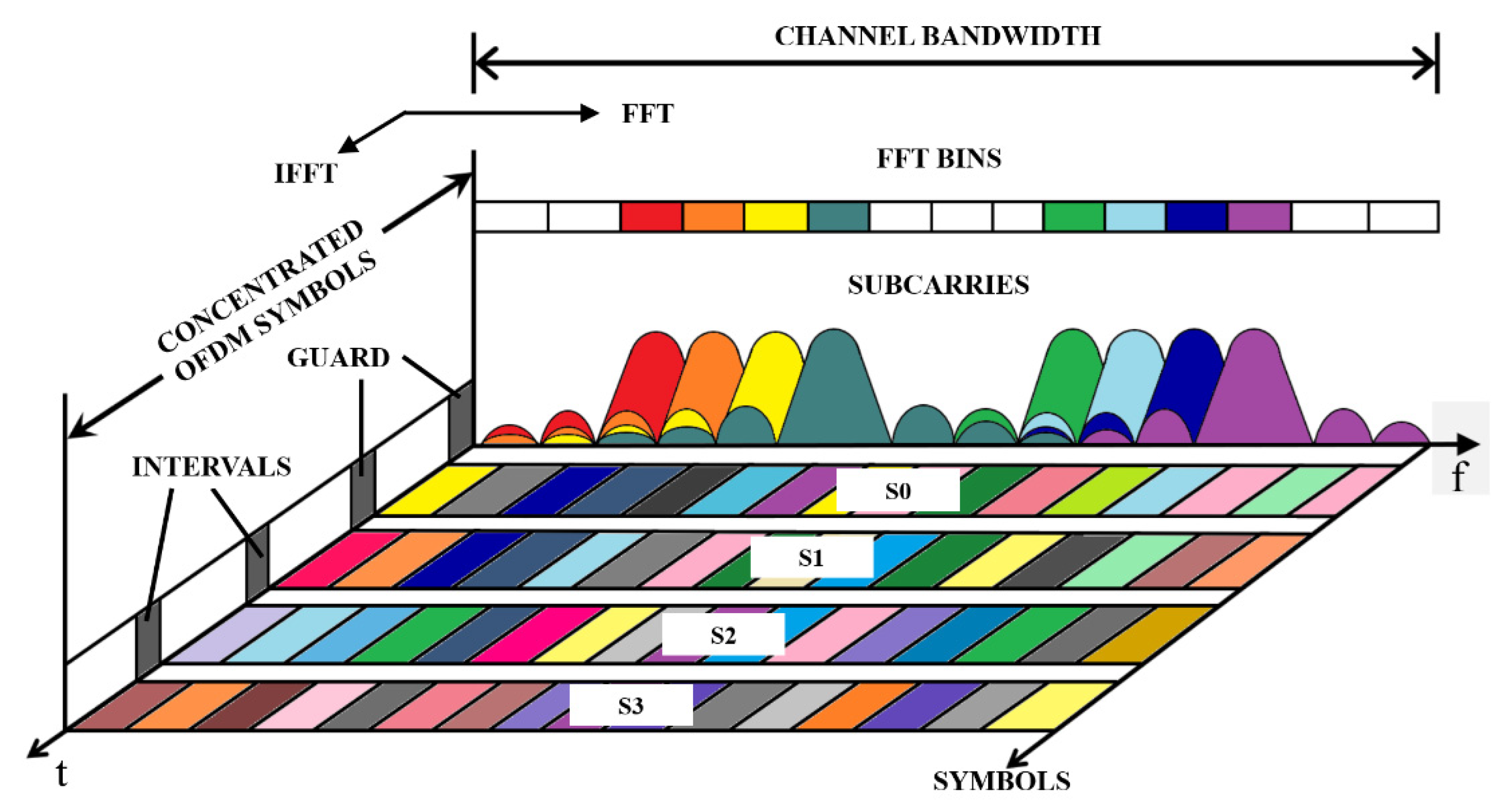


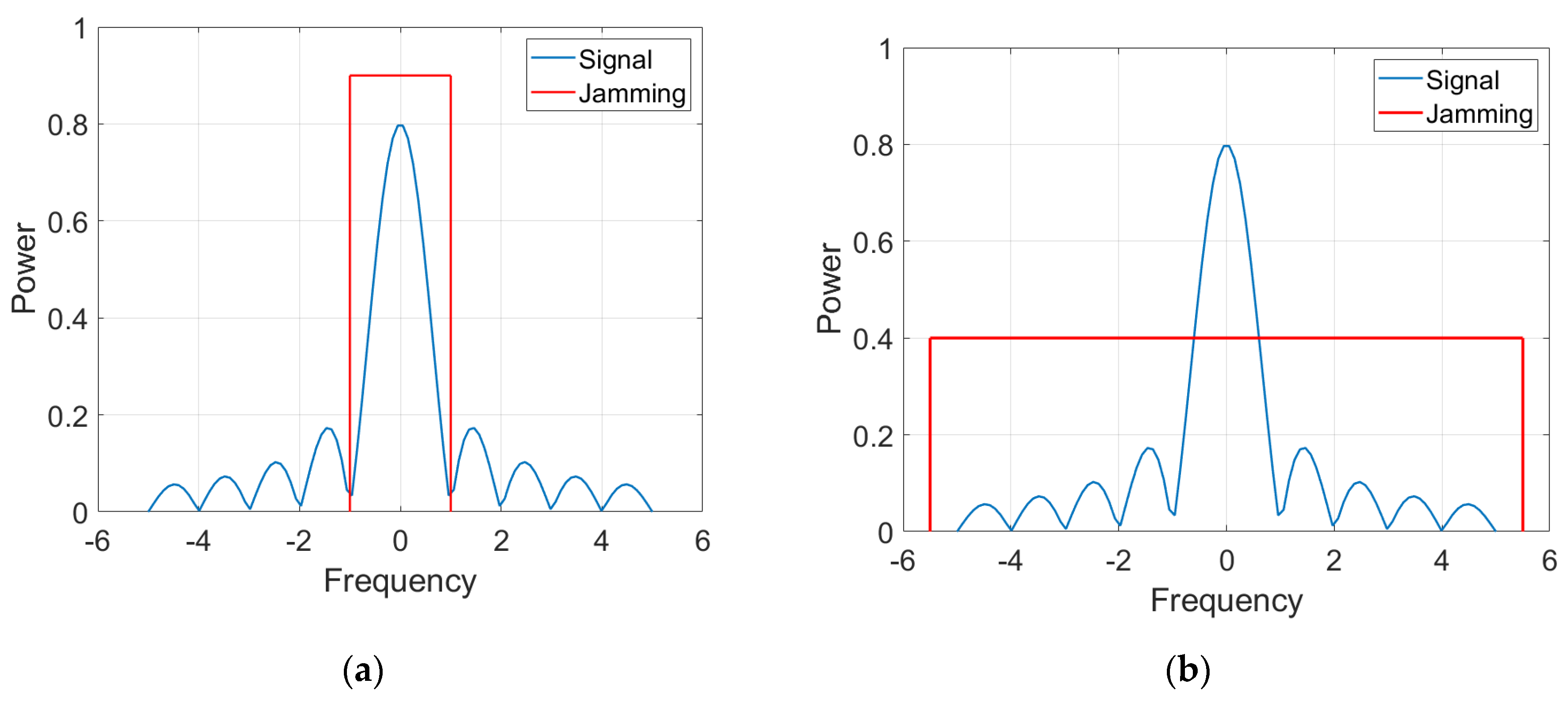

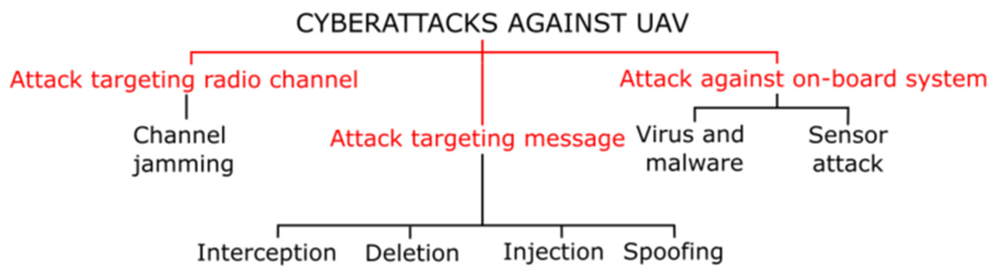
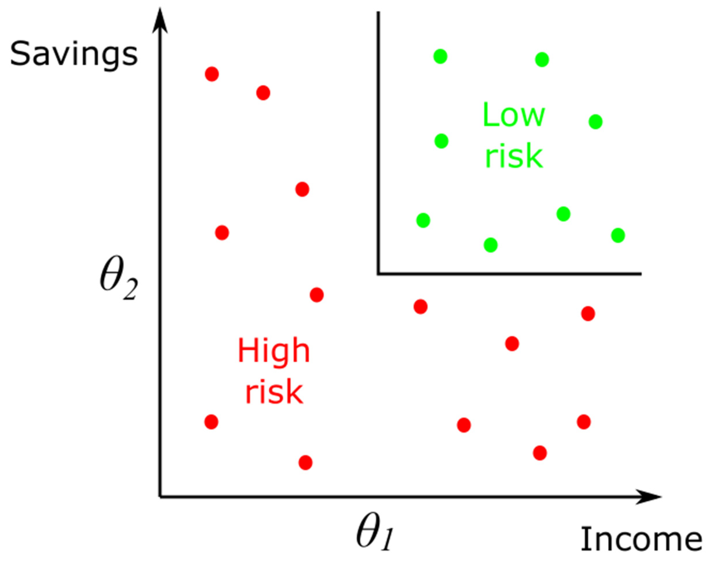
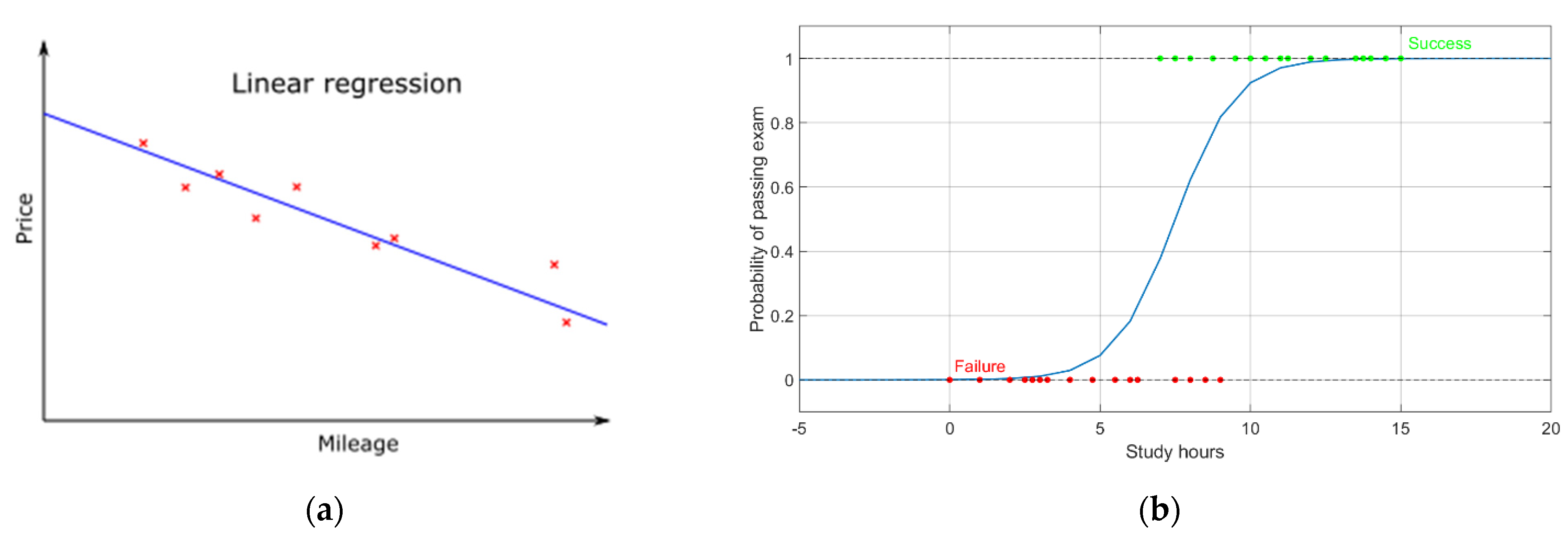
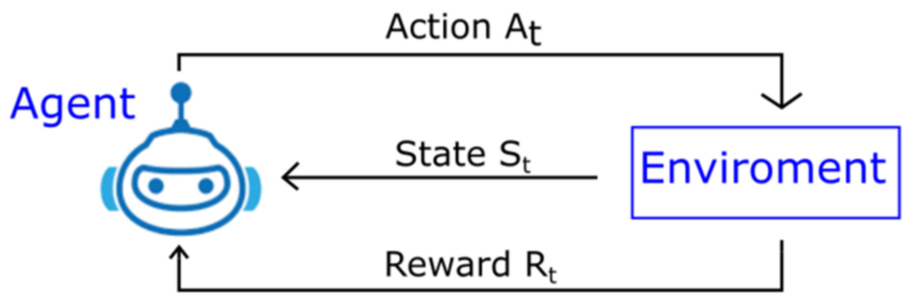


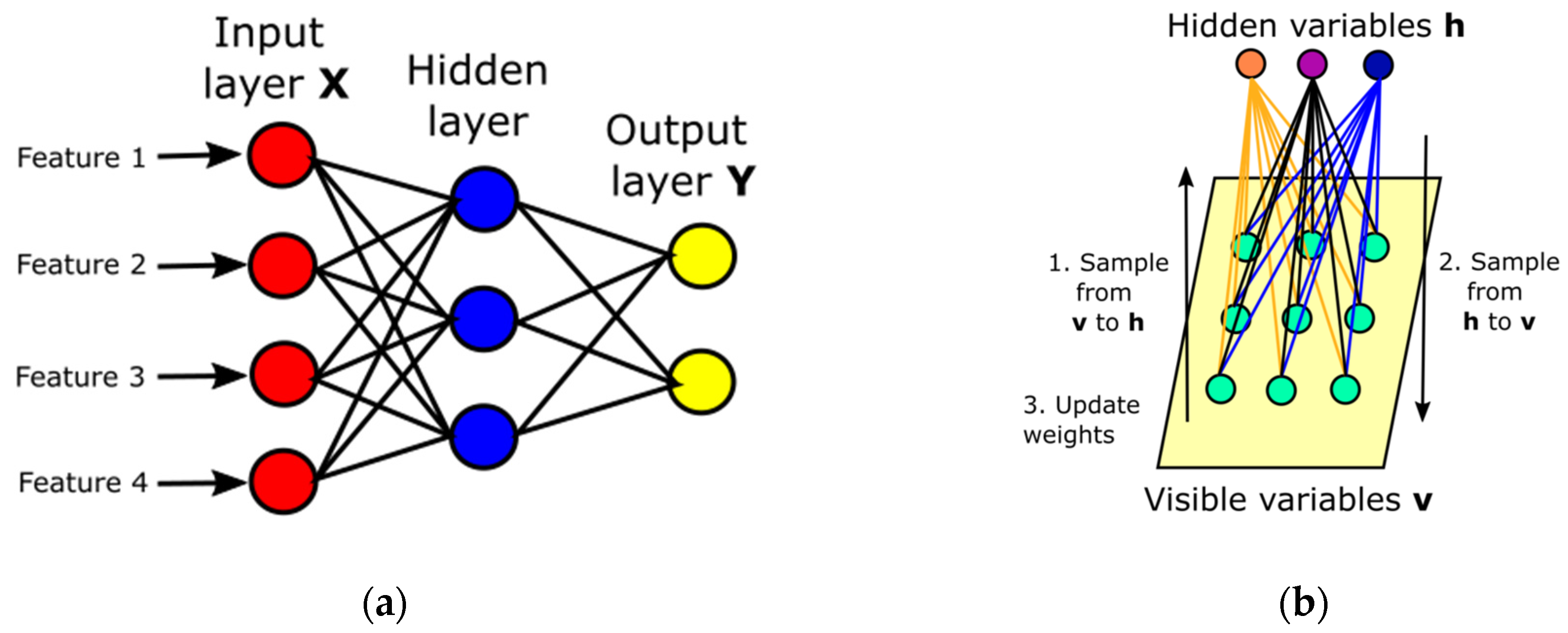
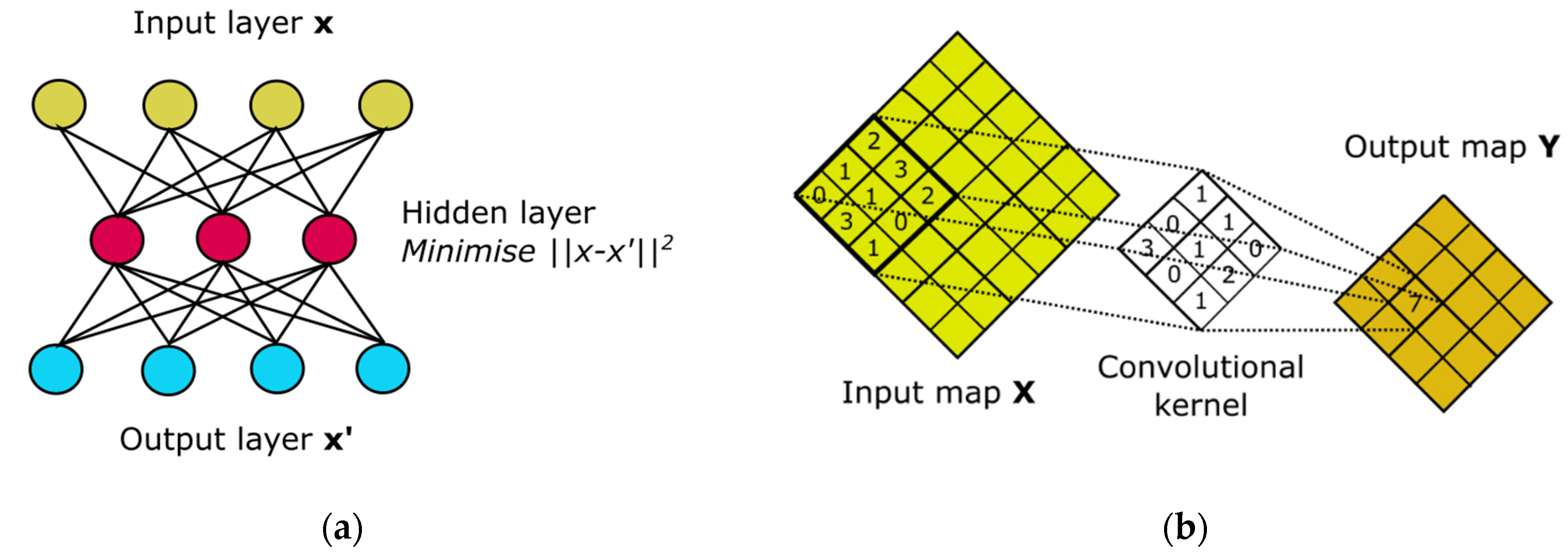

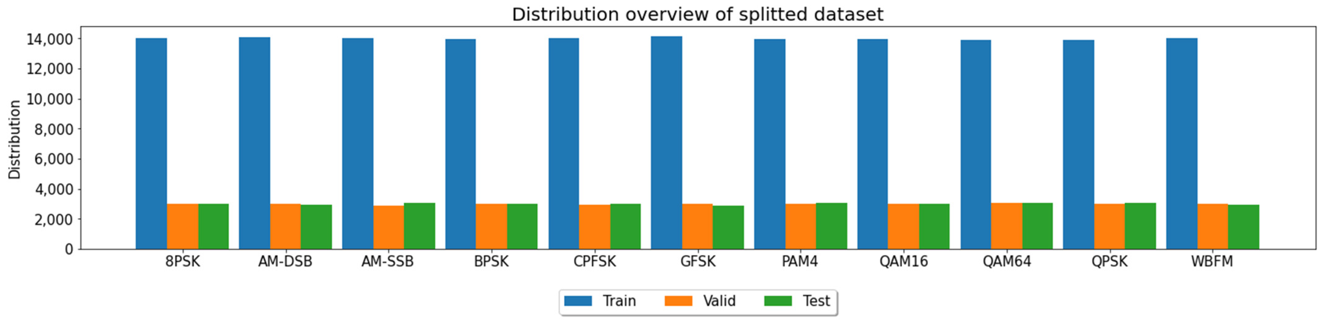


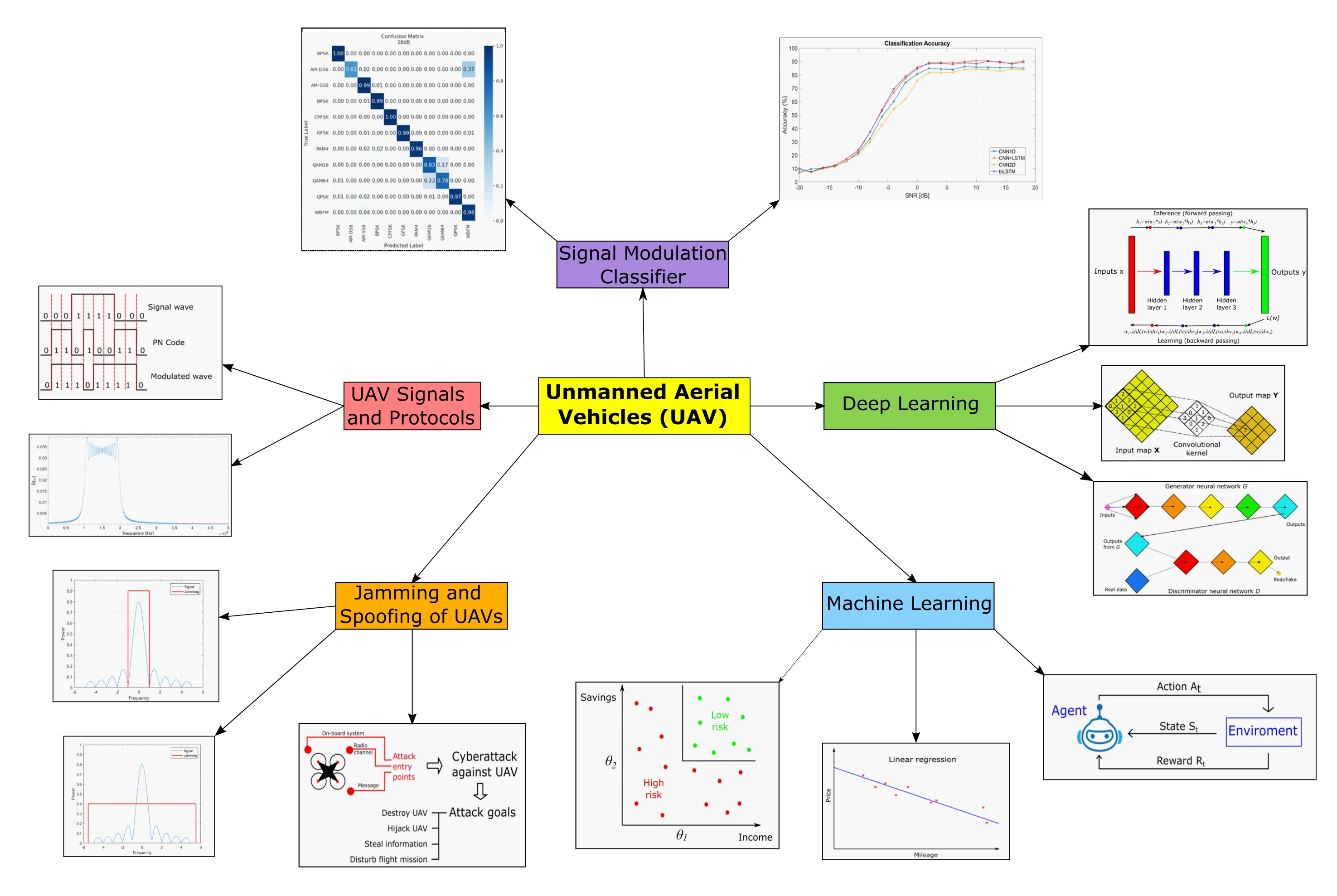
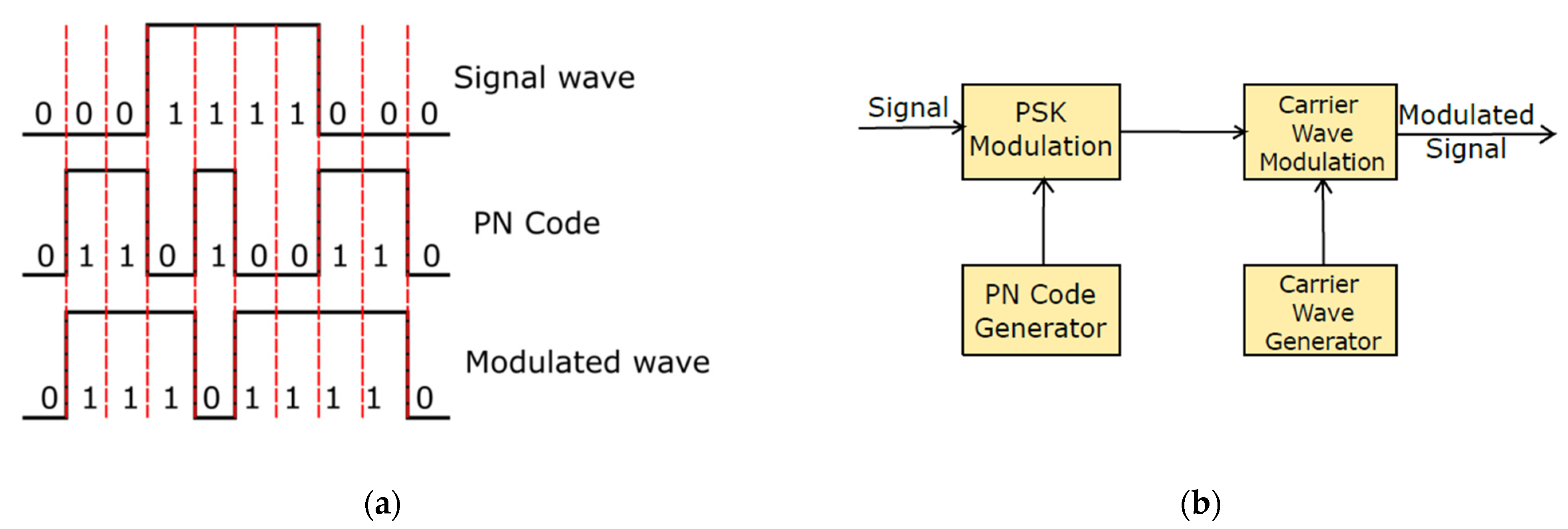
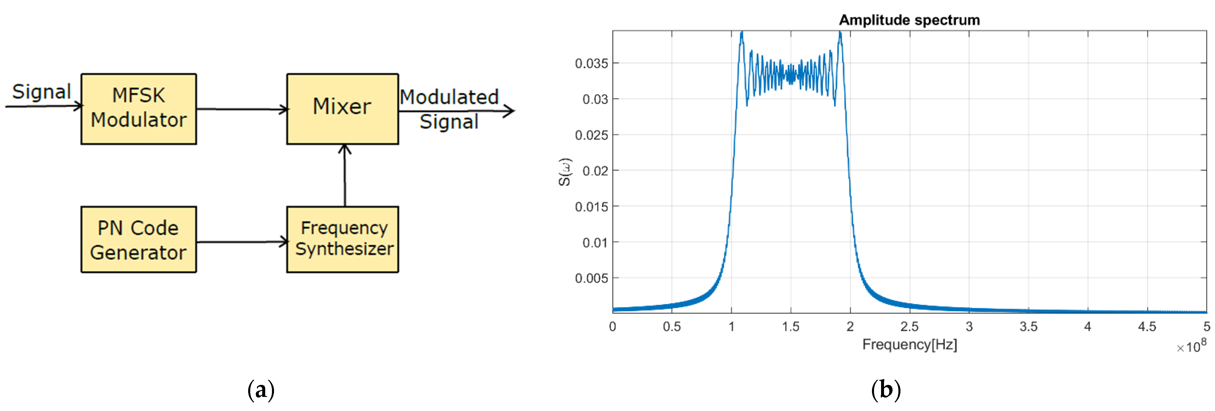
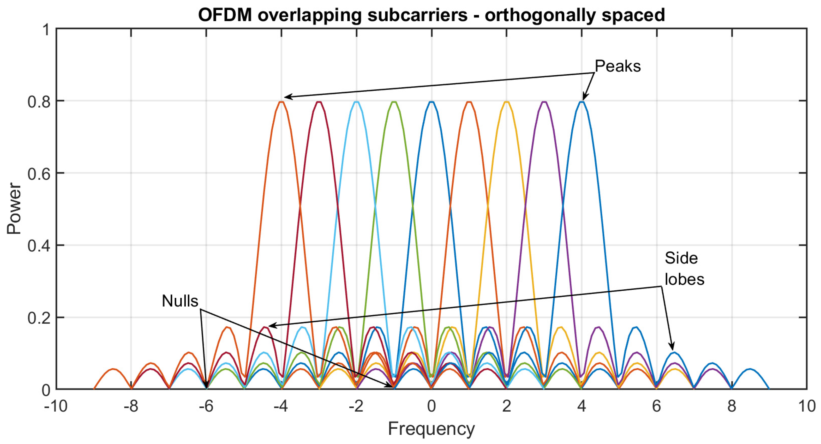
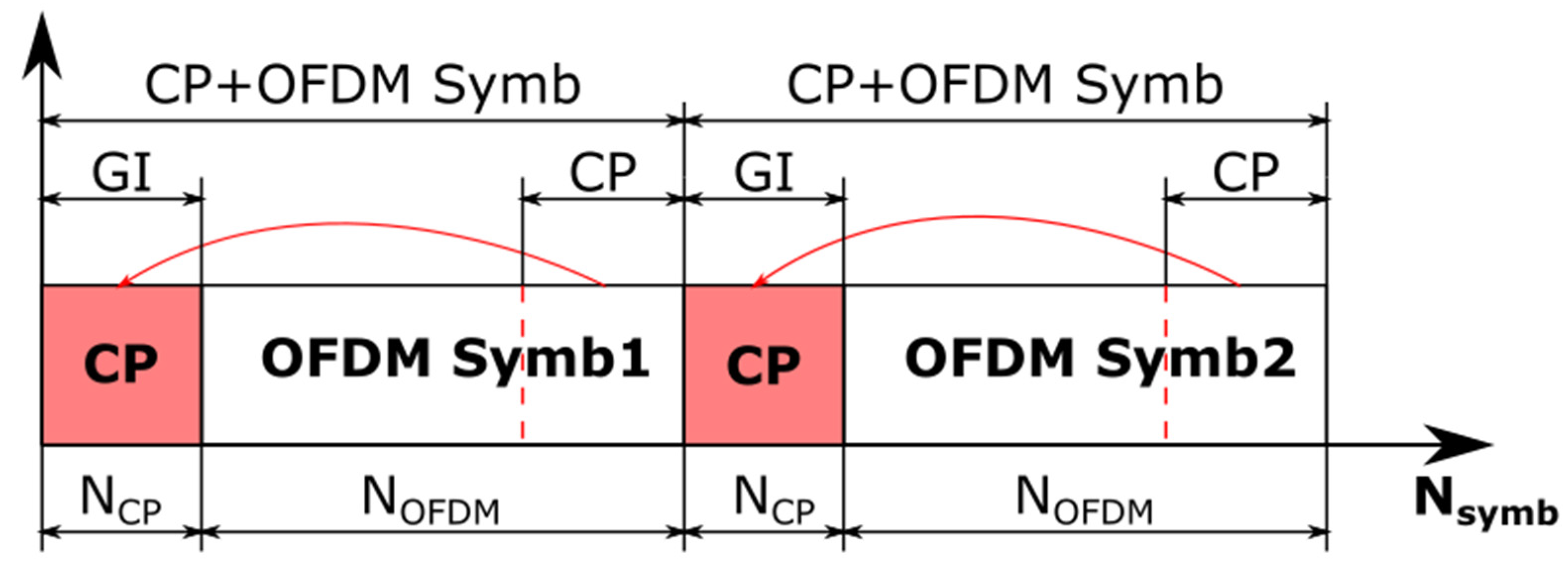
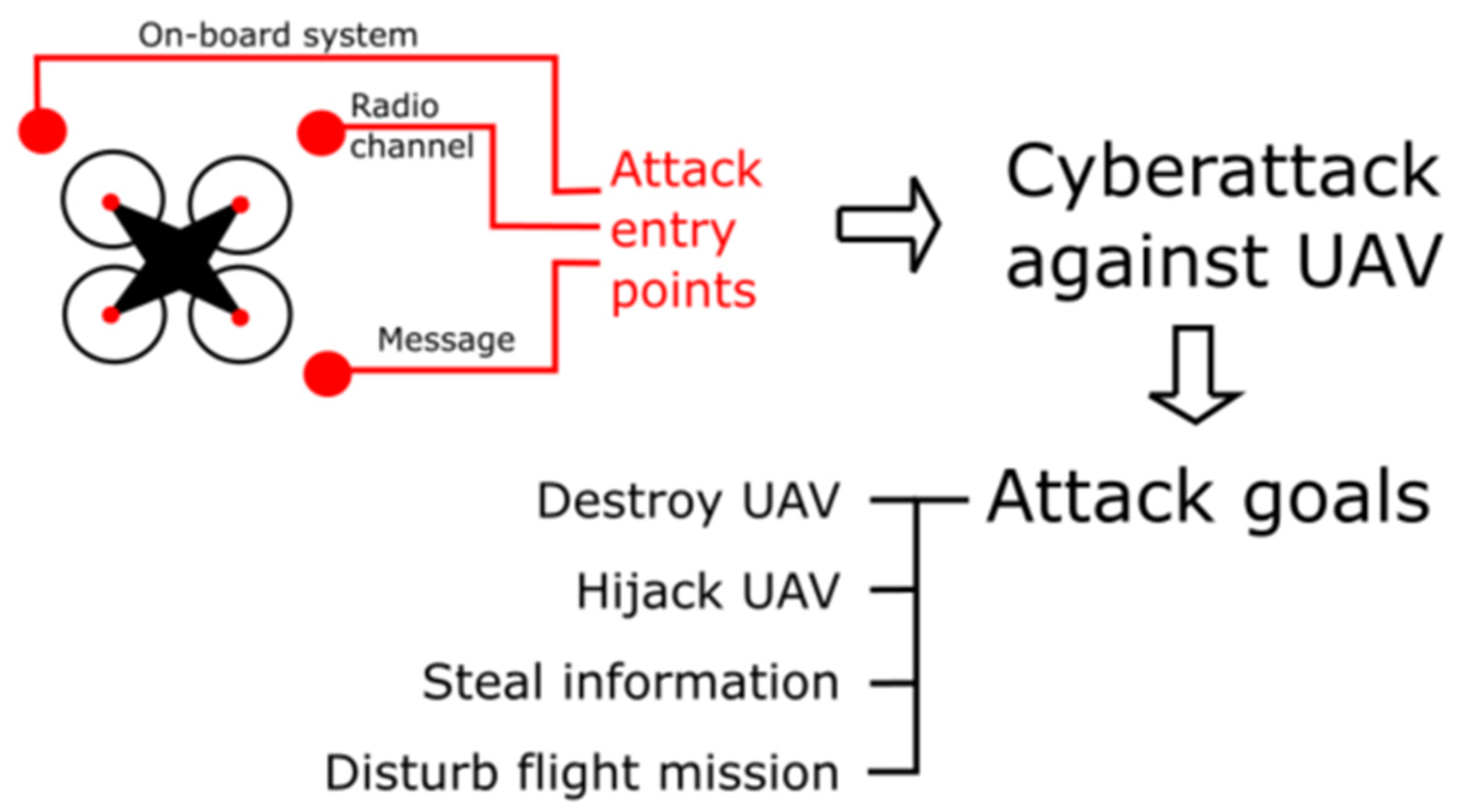
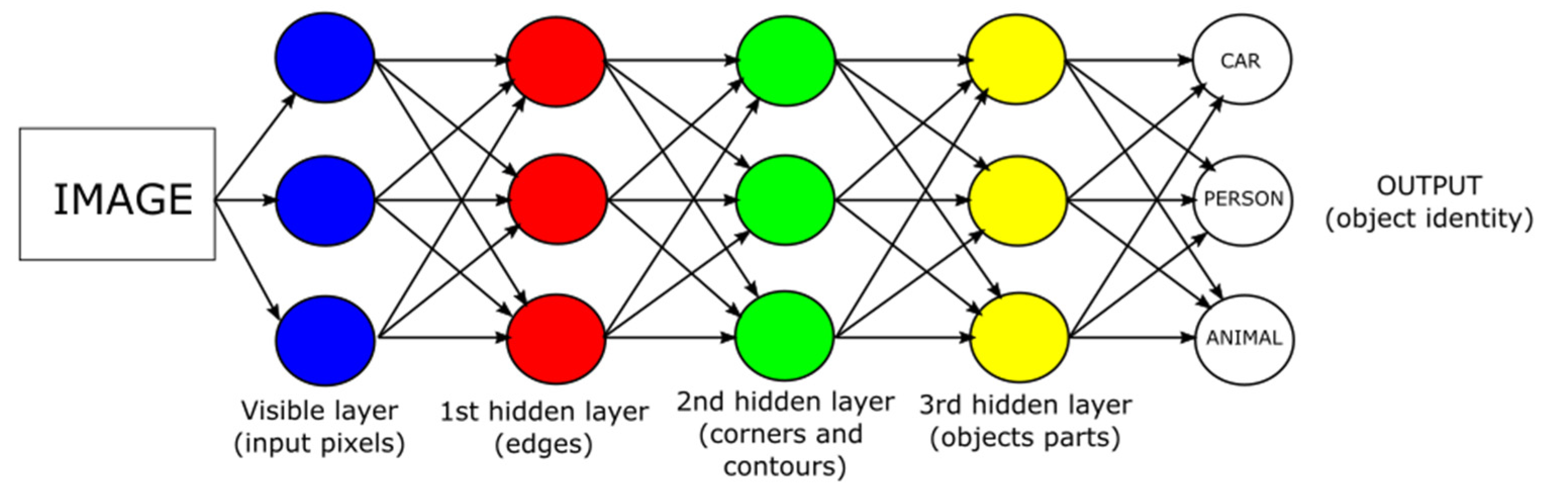
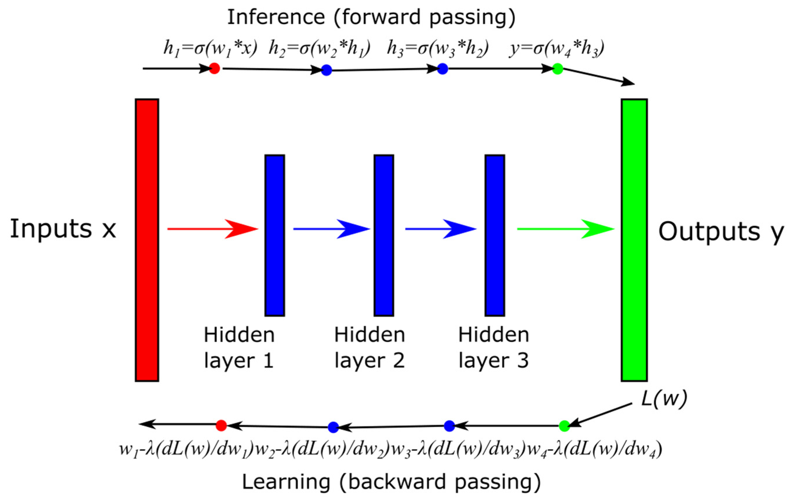
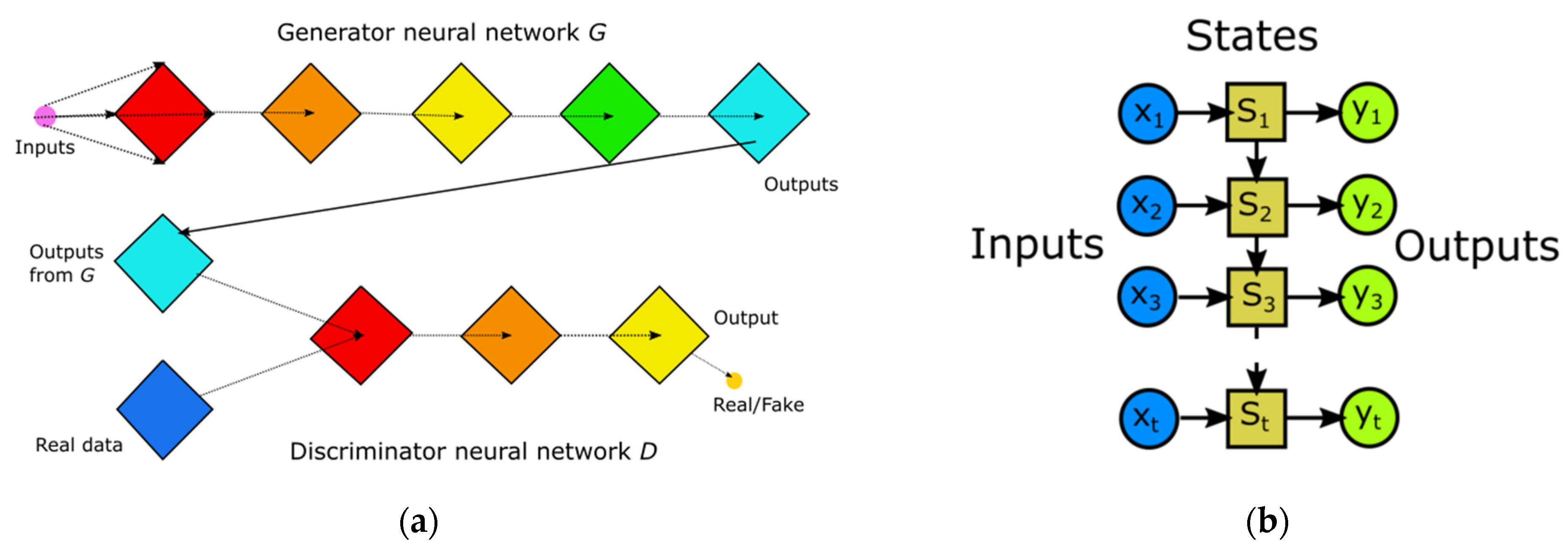
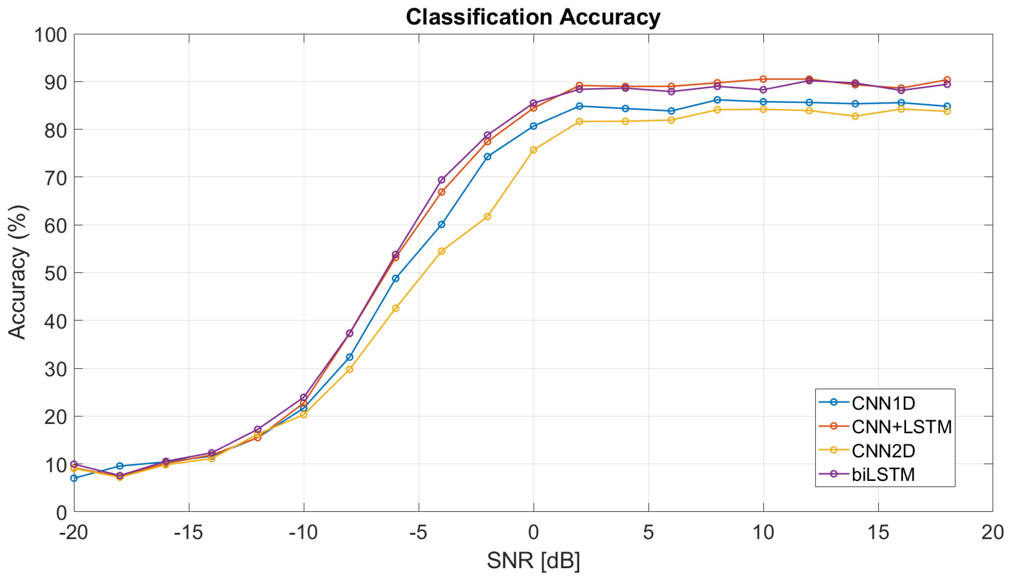
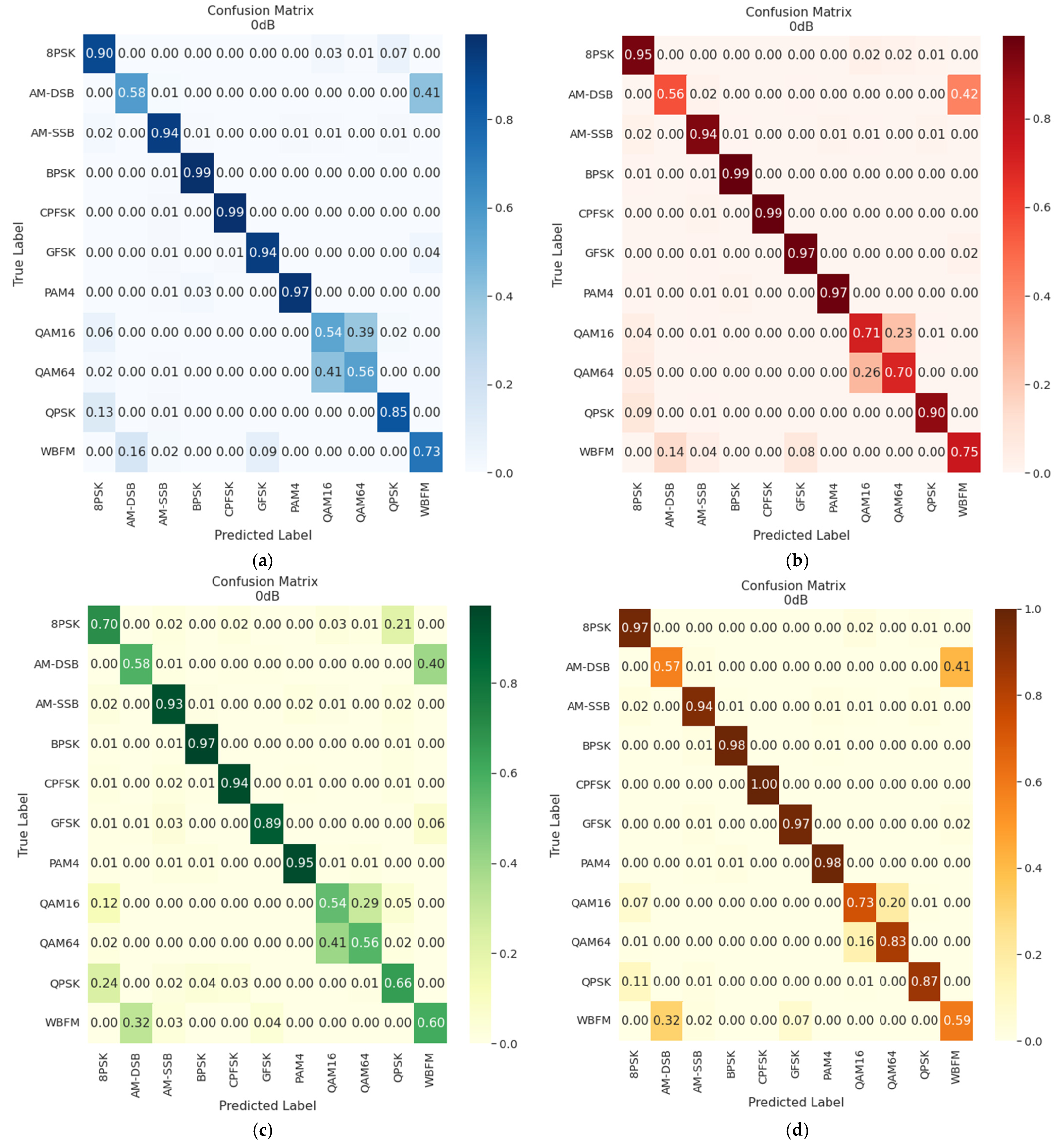
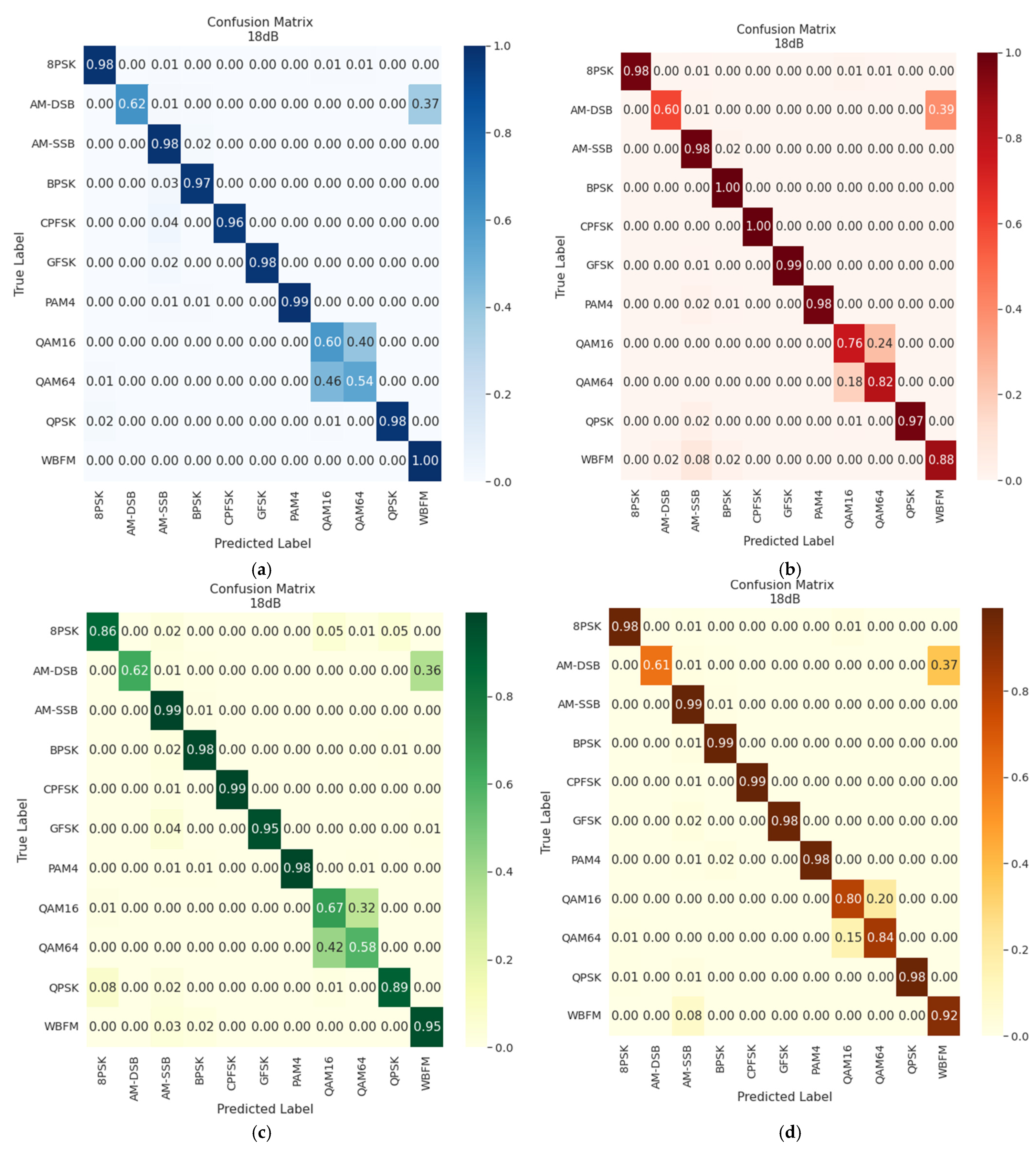