Lane following Learning Based on Semantic Segmentation with Chroma Key and Image Superposition

Abstract

There are various techniques to approach learning in autonomous driving; however, all of them suffer from some problems. In the case of imitation learning based on artificial neural networks, the system must learn to correctly identify the elements of the environment. In some cases, it takes a lot of effort to tag the images with the proper semantics. This is also relevant given the need to have very varied scenarios to train and to thus obtain an acceptable generalization capacity. In the present work, we propose a technique for automated semantic labeling. It is based on various learning phases using image superposition combining both scenarios with chromas and real indoor scenarios. This allows the generation of augmented datasets that facilitate the learning process. Further improvements by applying noise techniques are also studied. To carry out the validation, a small-scale car model is used that learns to automatically drive on a reduced circuit. A comparison with models that do not rely on semantic segmentation is also performed. The main contribution of our proposal is the possibility of generating datasets for real indoor scenarios with automatic semantic segmentation, without the need for endless human labeling tasks.

1. Introduction

The technology around autonomous driving is showing a considerable growth rate and is already in the integration phase as an innovation in society. It offers various possibilities for reducing accidents and the effort required in driving, among many other advantages.

Experimentation with autonomous driving started about a century ago and began to provide some interesting results in the mid-20th century. Some decades later, a few of the most renowned projects, such as ALVYNN [1] and EUREKA PROMETHEUS [2], were developed.

In the last decade, advances in alternative computing architectures oriented towards parallel computing have particularly benefited deep learning or image processing techniques that require intensive parallel processing. This has led to the widespread use of DL techniques in various fields, including autonomous driving [3].

Lane detection and following is a fundamental task that can be accomplished with classical methods or can benefit from combining methods based on deep learning and further pre- or post-processing [4,5,6,7,8,9,10,11].

The techniques on which autonomous driving systems rely can be distinguished based on the type of sensors they use, the information they collect, and the way they treat said information. In some cases, a large number and variety of sensors are used to infer, through the application of machine learning methods, some explicit characteristics that allow for taking appropriate decisions. This approach is typically called mediated perception [12] and is currently used by some of the most notable autonomous driving systems, allowing for route planning and more elaborate control. Another advantage of multimodal approaches that use multiple sensors is that they allow for solving situations in which some sensors do not deliver adequate information; for example, in the case of detecting the road by means of a camera in adverse weather conditions [13].

Other systems use only an input image and apply Computer Vision and deep learning techniques to interpret the image and determine the actions to be carried out.

Mapping the image pixels onto control actions gives rise to the Behavioral Reflex, which makes it unnecessary to understand the environment explicitly. Much work has been devoted to this approach, which is also known as end-to-end learning systems [14,15,16,17] and which consists of learning a behavior based on training the relation between the images recorded by a camera and the associated driving actions.

In general, imitation learning attempts to relate the data provided by different sensors to the actions performed in real time by a human driver. This has the advantage of providing an annotated dataset that is suitable for many machine learning or deep learning methods based on supervised learning. In this context, the car learns to drive by imitation of the behavior of the human driver. Alternative techniques that do not rely on annotated datasets and supervised learning can be applied based on reinforcement learning [17].

A more refined approach consists of using a two-phase learning system, in which a first frontend system is used to extract relevant features from the input images—in this case an Autoencoder Network, which is trained to output the same image as the input. This network performs a dimensionality reduction that allows it to codify the input image in the Latent Vector. This collection of values can be then used to train a backend system to learn to drive. The advantage of these systems [18] is a notable reduction in the computational cost. A drawback is that the encoding performed by the Autoencoder is not only focused on the characteristics of interest (the lines or the lane), but other elements of the images are also included in the encoding process and may disturb the final codification.

A further step towards improvement can be expected by training the frontend system to perform a semantic segmentation of the input image, i.e., to identify the kind of objects of interest that are present in the input image. This is used in numerous systems based on simulators [19] and allows a more human-like structured approach. The disadvantage is the dependency on the use of specific predefined scenarios, as very precise semantic labeling is required. To ensure the correct operation, it is important to validate the final model in real environments, where it is more difficult to perform a reliable semantic labeling procedure. In some cases, it takes a great effort to tag the images with the proper semantics. This is also a relevant problem given the need to have very varied scenarios to train and, thus, obtain a good generalization capacity [20].

In this context, a technique is proposed to automate the segmentation and semantic-labeling process based on the combination of scenarios with chromas and the superposition of images in indoor scenarios. Improvements in the segmentation process with additive noise techniques are also studied.

Applying semantic labeling to the elements in a scene is not an easy task. The use of Computer Vision techniques to segment or classify these elements can cause numerous failures. Manual labeling seems unfeasible because it is an excessively hard and tedious process.

Our proposal is based on building a scenario based on chroma that facilitates the segmentation of some basic elements, such as the lines or the road itself. For this task, we resort to techniques related to chroma key in an HSV color space. This process is quite easy to automate, and the isolated elements can be used to augment other indoor scenarios, creating new fictitious scenarios. These will then be used to train neural networks that must learn to perform the semantic segmentation of these elements and, then, to learn to drive automatically under the supervision of a human operator.

The approach discussed in this project proposes an alternative method to automate vehicle steering training without the need for driving simulators. The use of the chroma scenario allows to perform segmentations with the lowest possible failure rate, so that reliable labeled training datasets can be generated to learn the segmentation of road lines. Using a human driver to apply imitation learning has the advantage that his or her driving provides the equivalent of the ground truth annotation needed to apply supervised machine learning or deep learning algorithms to the input images. This also provides a simple way to evaluate the performance of the trained models, which can be compared to human driving.

The proposal is also based on the use of a small-scale vehicle model with a front camera that learns automated driving on a small-sized circuit. To obtain the labels that identify the key elements of the scenes and the associated control actions, it will be essential to have a human operator driving the vehicle and whose driving actions are recorded along the image stream.

The system is completed with an external computer and a control device (steering wheel), which allows for obtaining and storing the driving datasets to be used in learning. The computer and the small-scale vehicle communicate through wireless connection.

The structure of the document follows the scheme indicated below: the general idea of the proposal is presented in the Introduction; the Related Work section addresses the aspects of interest related to autonomous driving and neural networks; in the Materials and Methods section, the technical details of our proposal and the experimental design are described; later, the Experimental Results, and a Discussion of these results, are addressed; and lastly, the Conclusions summarize the highlights of the proposal.

2. Related Works

In this section, a review of previous work is given, focusing on Autoencoders, chroma-based image processing, and some previous applications in end-to-end autonomous driving learning.

2.1. Autoencoders

Autoencoders are neural models with two components (encoder and decoder) whose task is to learn the identity function, replicating the input data in the output [21]. A specific hidden layer, called a latent vector, will learn to generate a representation of the input data.

Undercomplete Autoencoders use hidden layers with smaller dimensions than the input and are useful to reduce the dimensionality of the input data. Only those characteristics that differentiate one entry from the rest are reflected in the encoding of the latent vector, thus achieving an extraction of relevant characteristics from the entry.

Stacked Autoencoders use more than one layer to facilitate both the encoding and the decoding processes, in the sense that they allow a progressive reduction in dimensionality. In this way, they manage to improve the representation of the data in the latent vector.

To improve the learning process and, specifically, the generalization capacity of the model, it is possible to apply different techniques based on regularizers. A particular case is the addition of noise at the input. This modifies the training instances and allows the dataset to be expanded. As a result, the trained network will improve its ability to generalize and its tolerance to noisy inputs, generating a more robust network [22]. In a general sense, training a network with noise promotes more neurons in the network to contribute effectively to its operation [23].

Denoising Autoencoders apply these techniques to remove noise from input data or to obtain more noise-tolerant models. One of the consequences of learning based on this noise is an improvement in the representation of the data in the latent vector and, thus, a better extraction of features [24] with the help of Stacked Denoising Autoencoders [25]. What is sought with this type of network is an improvement in the representations of the input data.

Combining these architectures with convolutional models results in Convolutional Autoencoders that are adequate for image processing [26].

One application of Autoencoders is the segmentation of images. In this case, the training datasets associate each input image with the corresponding segmented image, making it possible to obtain Autoencoders capable of performing segmentation [27]. Similarly, they can be applied to determine the area of interest of an input image. By training with output images in which only the elements of interest are present, it is possible to obtain a model that learns to isolate these elements in an input image.

2.2. Image Processing

The use of neural networks for image processing—in particular, with convolutional neural networks—is a widely accepted alternative to other classic image processing techniques. A drawback is that they require extensive datasets to train them adequately. This, in turn, requires the use of other techniques to prepare the necessary datasets.

Our proposal addresses this process with an alternative setup based on chroma key techniques and the HSV color model.

The chroma key technique [28] is applied by identifying a specific color in the image and replacing the area it occupies with another image.

Similar approaches based on chroma key separation are applied on semantic segmentation [29] for object detection [30,31] and the detection of the hands of drivers [32].

The HSV color model is useful to make selections in an image based on specific colors [33]. The colors are described in this model with three parameters: hue (H), saturation (S), and value (V). The hue parameter represents the color spectrum. Saturation determines the purity of the color, and value represents its brightness. This model allows comparisons of different colors with the use of simple techniques focused on the parameter H, which is especially useful for fast processing with chroma techniques.

In our proposal, the input images are segmented using chroma key techniques in the HSV color space. The segmented output is then used to generate fictitious images through the superposition with the images of an indoor target scenario. This method allows for creating an augmented dataset that will be used to train the neural networks.

2.3. Learning to Drive

Some previous works have addressed similar problems related to autonomous driving and are detailed here. Extensive and comprehensive surveys can be found in References [34,35].

Bojarski et al. [14] addressed the problem of learning to drive using a single convolutional network to process the images from a camera located at the front of a full-scale vehicle. The neural network generates a projection of the space of the images in the space of driving actions. This system has the advantage that the network itself learns to interpret the environment, and this is achieved based solely on the labels provided by the supervised driving without requiring prior processing. This work empirically demonstrates the possibility of learning the complete driving task using a DNN, without the need to resort to other methods to interpret the environment.

Yang et al. [18] proposed a Stacked Autoencoder to learn how to extract the necessary characteristics of a scene for the autonomous driving of a vehicle. The Autoencoder is trained in the first phase with each image at both the input and the output. In this way, the Autoencoder learns to code the relevant characteristics that allow an adequate reconstruction of the image. Subsequently, an additional neural model with three outputs is added following the latent vector of the Autoencoder, and this is trained using input images associated with three turn labels: left, right, and straight. As a result, the vehicle learns to travel in the circuit and with a changing environment, which reinforces the result that the network generalizes correctly, focusing on the characteristics of the circuit and ignoring those of the environment.

Other approaches are based on the use of classical image processing algorithms to detect road lines. A typical case could be a workflow based on the Canny edge detector, the result of which can be processed by the Hough transform and with some kind of regression to reconstruct the lines. An example is given in Reference [36]. Driving learning can be then based on the extracted features or on the generated image, applying algorithms that can include machine learning or deep learning. We will use an alternative based on the Canny edge detector to compare results with those based entirely on deep learning.

Our proposal follows those of References [14,18] in seeking to facilitate the location of the relevant elements of the scene and to encode them in a feature vector. Bojarski et al. [14] forced the learning algorithm to search for relevant elements among a set of all the details of the input image. The proposal [18] adds a feature reduction of the input space using an Autoencoder, which is expected to ignore the nonrelevant elements of the image.

Our work proposes to focus only on the elements (lines of the road) and perform a feature reduction on them. By focusing only on these, the Autoencoder will not be forced to encode irrelevant elements, so the quality of the feature vector should increase. This implies the necessity of precisely determining both their position and orientation in the input images. Our approach uses a first phase in which chroma key and image superposition techniques are used to generate an augmented dataset that serves to train the Autoencoder to simultaneously perform the semantic segmentation of the lines and their encoding in a feature vector. With the addition of input noise, some invariance is achieved, with issues of the nonmatching illumination in the image superposition.

Once the Autoencoder is trained, the driving learning task is easily completed under the supervision of a human driving operator.

3. Materials and Methods

This section deals with the design of the proposed solution and its contribution with the use of an artificial chroma stage. This will facilitate the segmentation of relevant elements in the driving scenario—in this case, the lines and the road. For the training phase, it will be important to extract only the features corresponding to those lines. Another application of this setup will be the application of this method to the generation of superposed images to allow a virtual training of the network in indoor scenarios.

A detailed description of the experimental setup is also given.

3.1. Solution Design

Here, we describe our proposed solution, which consists both of a working environment and the operating procedure. The additional needs include the design of a small-scale vehicle and of a control system that allows the car to be driven remotely and to collect the driving data for training purposes.

3.1.1. Small-Scale Vehicle

To perform and validate the tasks of this project, a small-scale vehicle is developed. A wide-angle camera (160° viewing angle, 5 megapixels) is placed at the front end of the vehicle.

A steering axle controlling the two front wheels of the car ensures a more realistic driving style. Two synchronized DC motors provide the traction of the vehicle on the rear wheels.

A Single Board Computer (SBC, a Raspberry Pi 3B+) will handle the necessary processing, which includes initial image processing (image scaling), streaming to the external computer that stores the data and performs the training of the neural models, receiving the driving orders, and the control of the steering and traction of the wheels. Once a trained model is transferred to the SBC, it will be able to perform the necessary inference to drive automatically.

3.1.2. Working Environment

A key task is to isolate the road lines from the input images, discarding the other elements. This is a difficult task in real environments. Therefore, we propose the use of a special scenario based on chromas. The materials are selected carefully to allow for the application of the chroma key technique in an HSV color space.

OpenCV [37] has been used for applying color masks to identify areas of interest in an image based on color similarity. Table 1 includes the boundary values used for masking out each chroma. In OpenCV, the value range for the hue channel is (0, 179), whereas both the saturation and the hue values are in the (0, 255) interval.

Table 1. Boundary values used for the chroma masks.

Chroma	Hmin	Hmax	Smin	Smax	Vmin	Vmax
Green	69	89	123	255	85	255
Red 1	160	179	81	255	91	255
Red 2	0	16	81	255	91	255

The working environment consists of the following elements, shown in Figure 1:

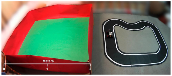
Figure 1. Components of the complete working environment. Depending on the required task, the driving circuit will be placed either in the chroma scenario (left) or in the target scenario (right). The driving circuit can be placed in either stage when needed.

• Driving circuit—A track is designed by placing white lines on black cardboard that imitates asphalt. To facilitate the supervised driving and the learning tasks, the track forms a closed loop.
• Target stage—The final learning task is performed in this stage. It serves as the real-world stage.
• Chroma stage—The design of this stage is based on elements with easily separable colors. When the driving circuit is placed inside of this stage, it will be possible to process the captured images to extract either the road or the lines of the road. The isolated road can be combined with the target indoor scenario for training purposes. The following section gives a more detailed view of this process.

3.1.3. Operating Procedure

The two main tasks of this problem are feature extraction from images and the use of these features in the process of learning to drive. A camera placed at the front of the vehicle provides a stream of images as input for the automated driving system. This system must extract the features corresponding to the road lines and then use them to control the steering of the vehicle. The expected output of the driving system is the required steering angle. Both tasks are solved using artificial neural networks trained with supervised learning. Figure 2 shows a diagram of this system.

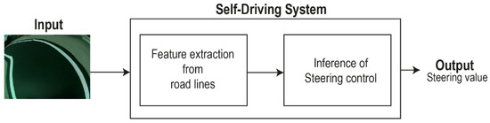
Figure 2. Self-driving system schema.

The usual alternatives for dealing with these tasks are using either real scenarios or computer-simulated scenarios.

-

In a real scenario, accurately segmenting the lines or other elements is complicated, and errors occur that can compromise the results.

-

In a simulator, a generative method can be applied, creating a scenario in which the situation of the relevant elements (the lines) is precisely known [15]. However, in this case, it will be more difficult to achieve realistic images.

Another usual approach is to rely on both resources: training a neural model with data provided by a simulator and testing it on real-world scenarios [15,16,17,38].

Our proposal is to apply ideas from both cases. Instead of using a simulator to generate scenarios, we rely on an artificial scenario that simplifies the segmentation of the road lines, which can be combined with an indoor scenario. The whole training process is performed in four phases (Figure 3 illustrates this process):

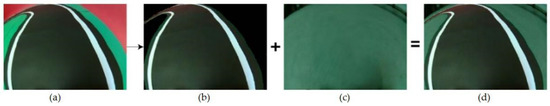
Figure 3. Processing flow for generating the superposed images. The image (a) is captured in the chroma stage. By applying color masks on the image (a), the road is isolated (image (b)) and superimposed on the image (c), which has been captured in the target environment. The superposed image is (d).

• In the first phase, the road will be placed in the chroma scenario, and a human operator will drive the model car within it while the front camera takes a sequence of images. The image stream is processed in the external computer by segmenting the road and the lines from each image using the chroma key technique. This allows the generation of a dataset with the extracted road and lines.
• In the next phase, the model car will be driven in a roadless target scenario to provide a stream of images. The images with segmented road and lines from the previous phase will be superimposed on these new images, creating an augmented scenario. The superposed images paired with the images of the extracted lines will form a new dataset that will serve to train an Autoencoder, which is expected to learn to perform semantic segmentation on the images from the working scenario.
• In the third phase, the car is placed in the target indoor scenario (as shown in Figure 1) that includes the road, and the human operator must drive the model car again. The encoder part of the trained Autoencoder model will process the image stream from the front camera, giving at the output a set of values from the latent vector that describes the road lines. This time, the aim is generating a dataset that associates the values of the latent vector with the steering angle recorded while the operator is driving.
• In the last phase, an MLP is trained with the dataset generated previously. The combined model with the trained encoder and MLP is then transferred to the Single Board Computer (SBC) in the model car, allowing it to drive automatically.

3.1.4. Control and Training Data Collection System

In the training phases, the system must allow the remote and supervised control of the vehicle through a driving device (a steering wheel) and real-time video streaming. This will also allow us to build training datasets based on the pairing of each driving image and the corresponding recorded steering angle.

The elements required to deal with the tasks of the project (shown in Figure 4) are described below. In video 3, this system can be seen in operation [39].

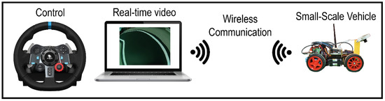
Figure 4. Control and training data collection system scheme.

• Create a wireless connection between the computer and the vehicle.
• Use of a steering wheel connected to the computer for remote control of the vehicle.
• Send control orders from the computer to the vehicle, mostly steering values.
• Real-time streaming of the images from the front camera of the car to the computer.
• Saving the images of the image stream and the steering angle values to create the datasets.

3.2. Experimental Setup

This section deals with the two main tasks of the present work, starting with the experiments that extract the road lines and obtain their feature vector from the latent vector. Next, the required experimental setup that deals with the task of learning to drive is illustrated. First, some technical issues are mentioned.

3.2.1. Initial Experimentation and Some Encountered Problems

The first issue related to the low inference rate delivered by the SBC, which was able to process only 2.5 image frames per second, determines the final design of the neural network architecture used and the size of the images to be processed.

Another issue was related to the vehicle’s useful speed range. This should be able to reduce the speed to a specific minimum without losing torque and, at the same time, have an acceptable maximum speed. This issue required the selection of appropriate traction motors.

A final issue was related to the angle of view of the camera. Despite having an extreme wide angle (fisheye) lens, in many situations, it was not sufficient to frame both lines of the road at the same time. This issue required placing the camera to enable a high-angle shot.

3.2.2. Feature Extraction from the Road Lines

This task is referred to as the line extraction task and consists of training an Autoencoder to segment the lines of the road contained in the input images, ignoring the other elements. The latent vector of this network will hold a codification of these lines. The network (Figure 5) will be trained using the following setup:

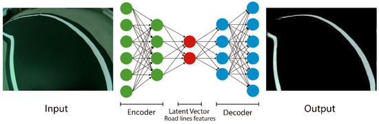
Figure 5. Line extraction task with the Autoencoder network.

In the first phase, an operator drives the vehicle on a circuit in the chroma stage following the image stream delivered by the camera. These images are processed using the chroma key technique applied in the HSV color space. This phase delivers output images containing either the lines or the road with the lines.

In the second phase, the car is driven on the target scenario without the road while its camera captures images. The process in this phase adds the output images of the previous phase (segmented road with lines) to the input stream from the camera (as shown in Figure 3), delivering superposed images.

Feeding these superposed images to the input of the Autoencoder and using the output images of phase 1 as the target (only the segmented lines) serves to train it to extract only the road lines from the images. Figure 5 shows a diagram of this setup.

The set of images taken in the chroma stage (see Figure 6a) contains 9909 images. Of these, 45% are driving sequences in both directions on the road. The remaining 55% correspond to arbitrary driving, which will provide images of the road from varied perspectives. The training set is built with 6937 images, leaving the remaining 2972 images for the test set.

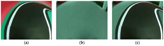
Figure 6. Example of the dataset built with image superposition. (a) Image captured in the chroma stage. (b) Image taken in the target scenario. (c) Image superposition (a,b).

All of these are processed to extract the road lines, which are needed for feeding the output of the Autoencoder in the training phase. A similar process extracts the road with the lines, which is then used to generate the augmented dataset.

A total of 4451 images are taken in the final scenario without the road. These are combined with the images of the isolated road with the lines, as shown in Figure 6. The combination of both sets of images generates a final training set with a high cardinality, which benefits the generalization capacity of the Autoencoder.

The initial image size of 640 × 480 pixels is later resized to 320 × 240 or 160 × 120, depending on the experiment. The smaller-sized images allow for a faster inference process in the SBC, which is important for avoiding driving failures with the model car. The question remains as to whether downsizing may compromise driving due to resolution or image quality issues.

The used Autoencoders have the following structures and parameters:

• A set of four convolutional layers, each one with 32, 64, 128, and 256 filters and each followed by a Max-Pooling layer;
• A latent vector of 32 values;
• Training is performed with the Stochastic Gradient Descent and the Binary Cross-Entropy Loss Function, with a batch size of 32 and lasting 100 epochs;
• A Gaussian noise layer is included to allow experimentation with the input noise with a standard deviation between 0.0 and 0.5. This layer is used with the training process to increase the quality of the reconstructions;
• The deconvolutional layers are designed symmetrically with the encoder.

The results of these experiments are shown in the Experimental Results section.

3.2.3. Learning to Drive

For the task of learning steering control, a densely connected network (MLP) is used to process the features extracted by the Autoencoder rather than using an image as the input. The dataset for this task is collected while driving with the circuit placed in the target scenario.

To build this driving model, only the encoder part of the Autoencoder is used, which extracts the characteristics and generates the latent vector from the captured image. This feature vector is used as the input of the MLP, which acts as a decision network. The target is the steering angle, which is represented as a linear value in the interval (−1, +1). During training, the modification of the weights of the Encoder is disabled. The structure of the complete network is shown in Figure 7.

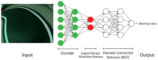
Figure 7. Graphical representation of the complete driving network.

The first set of data is obtained by following the route of the circuit in both directions. A total of 23,122 driving frames were captured as the result of driving about 6 min in each direction. This set (dataset DR1) is divided into two parts for training and for testing purposes. The images are later resized to either 320 × 240 or 160 × 120, depending on the needs of the used Autoencoder. More details of the distribution of the dataset are shown in Table 2.

Table 2. Distribution of the frames in the datasets for the driving task. The images are later downsized to 320 × 240 or 160 × 120.

Data Set	Size	Train Left	Train Right	Test Left	Test Right	Train Total	Test Total
DR1	640 × 480	9.345	9.287	1.925	2.565	18.632	4.490
DR2	640 × 480	9.804	9.738	1.456	1.530	19.542	2.986
DR3	640 × 480	-	-	1.024	1.024	-	2.048

In the initial experiments, some problems were detected that could be attributed to the driving style. Therefore, a second dataset (DR2) is generated using a similar setup and distribution. In this case, a more precise driving style is used, keeping the model car close to the outside line and trying to take turns smoothly. This allows it to more consistently keep both lines in the camera frame.

To carry out a more precise final evaluation, a third dataset (DR3) is generated using a different circuit layout. A total of 1024 frames taken while driving in each direction are selected to obtain a balanced set.

The characteristics and parameters of the used MLP are the following:

• A set of five densely connected layers, each one with 512, 256, 128, 64, and 1 nodes.
• Each dense hidden layer is followed by a dropout layer with a parameter value of 0.2.
• A ReLU is the activation function for all the layers except for the output, which has a linear activation function.
• The output codifies the expected steering angle, which is represented as a continuous value in the interval (–1, 1).
• Training is performed with the Stochastic Gradient Descent with batch size of 32 and the Loss Function Mean Squared Error, which lasts for 100 epochs.

Once the network has been trained, the model is transferred to the vehicle to test the operation. A constant minimum speed is set, and the driving model is started.

3.2.4. Comparisons

To verify the correct operation of the system and its improvement with respect to the state of the art, comparisons with other systems have been made.

First, the proposed model is compared with another end-to-end model that is not based on semantic segmentation; that is, no module is trained to explicitly identify the lines of the road. In this case, a convolutional network with the same structure of the proposed encoder + MLP is used, similarly to the proposal in Reference [14]. This model is trained using the images at the input and the steering value at the output.

Second, the same model as in Reference [18] is used on the original images; in this case, the Autoencoder is trained to approximate the identity function using the same image at both the input and the output. The final model is built using the encoder and an MLP to determine the needed steering value.

Finally, a comparison is made with a road line detection system based on traditional image processing. In this case, the processing is integrated with the use of a filtered Canny edge detector, the Hough Transform, and a regression to reconstruct the lines. A discussion on this approach can be found in Reference [36]. The result will generate images that will be used to train the same CNN+MLP as in the first alternative comparison. This provides the benefit of having the semantic labeling for the initial images, which will facilitate the evaluation of the line detection.

The results of the experiments are shown in the next section.

To carry out the work, a computer with an i5-9400f processor, 32 Gb ram, and two rtx2070 gpus was used, with tensorflow 1.13.1 and keras 2.3.1 on ubuntu 18.

4. Experimental Results

This experimentation section deals with the two main tasks. Complementary details of this section are shown in the repository for this project [39].

First, the main experimentation process carried out to obtain the feature vector that describes the isolated road lines is illustrated. Second, the automated driving learning task will be described. The final experiments will serve to validate both learning tasks.

4.1. Line Extraction Task

This task serves to train an Autoencoder to focus on the relevant elements in the image and to ignore other elements—that is, to extract only the lines from the road coding their form and orientation in the latent vector of this network. The schema already described in Section 3.2 and represented in Figure 5 will be used, enabling the system to take images of the circuit in the target scenario and to extract the lines from the road.

Initial experiments were performed to determine the adequate parameter settings. It was found that the reconstruction capacity of the Autoencoder was notably improved by including a certain amount of input noise in the training process. The lighting changes in the different scenarios employed to build the datasets can be compensated for with this input noise addition, which delivers a more tolerant model. By testing different input noise distributions with an increasing standard deviation, a progressive improvement was obtained. The best reconstruction capacity is achieved with a standard deviation of 0.4, and this degrades progressively from the value of 0.5 onwards. Therefore, a standard deviation of 0.4 was chosen for training a more robust Autoencoder (improvements shown in Figure 8 and video 4 [39]).

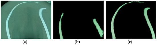
Figure 8. (a) Input Image from the target scenario. (b) Reconstructed output for the Autoencoder trained with input noise std_dev = 0.0 (c) Output for std_dev = 0.4.

Another experiment deals with downsized images. Based on the dataset with images sized at 320 × 240 pixels, a new set is generated with a resolution of 160 × 120 pixels, intended to accelerate the inference process in the SBC. Figure 9 shows that both the training and the validation errors decrease slowly after a rapid descent at the beginning of the training. Although the training lasts up to 100 epochs, a good convergence is achieved in the first 40–50 epochs. The learning process and the reached errors are similar for both image sizes.

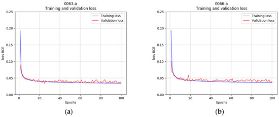
Figure 9. Descent of the loss functions for the same dataset resized to different resolutions. (a) Image size 320 × 240. (b) Image size 160 × 120.

There are no relevant differences in the values of the loss function when comparing both resolution sizes. The results obtained with the network generated in the previous experiments are quite good (for example, see Figure 10).

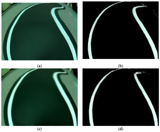
Figure 10. Camera images in the target stage vs. decoded output. (a) Captured in the target scenario 320 × 240. (b) Output of the Autoencoder 320 × 240. (c) Captured in the target scenario 160 × 120. (d) Output of the Autoencoder 160 × 120.

4.2. Driving Learning Task

This section will describe the experimentation carried out on the driving learning task—in this case, the steering of the vehicle.

The neural network used in this part relies on the feature vector delivered by the encoder part of the trained Autoencoder to learn the required steering value. Learning to drive takes place in the target scenario, with supervised driving sequences that serve to build a dataset by pairing both the captured image and the steering value.

One of the advantages of dividing the work into two tasks (extraction of features and learning to drive) is that the decision network (MLP) will have a smaller input, with fewer weights, making training easier and faster.

The network will be trained with the values from the latent vector as the input and the steering angle as the target. In this way, it will be possible to determine whether the network is capable of learning to infer the adequate steering angle from the characteristics of the lines.

The first experiment uses the network described in Section 3.2. In this case, the metric used is the error given by the Mean Squared Error function (MSE). For comparison, both image sizes are used to train the MLP, coupled with the corresponding encoder. Figure 11 shows graphs with rapidly decreasing errors.

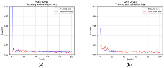
Figure 11. Evolution of the error loss functions. (a) Image size 320 × 240. (b) Image size 160 × 120.

Each MLP relies on the corresponding encoder part trained for images sizes of 320 × 240 or 160 × 120. Both cases reach convergence in the epoch range 40–60, with very similar evolutions and loss errors.

Once the models have been trained, they are transferred to the vehicle to test the driving operation.

When testing the driving models, the vehicle has difficulties in following the road when using images of size 320 × 240. This is mainly due to the poor inference rate (2.5 frames/second). The driving model using 160 × 120-sized images improves overall but still loses track on some occasions. This problem could be related to the driving style used for the supervised training.

The scatter plots in Figure 12 show the correlation between the expected steering angle and the real output of the driving model, using both the training and the validation set for the case of images sized 320 × 240.

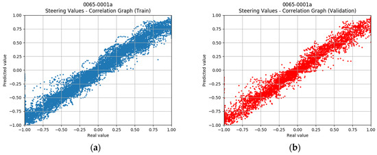
Figure 12. Correlation graphs for the expected vs. the predicted steering angle, images sized at 320 × 240, and the dataset DR1. (a) Scatter plot for the training set. (b) Scatter plot for the validation set.

With an ideally trained model, the scatter plots should show a thin straight line following the identity function. In the real world, one difficulty is that the decisions of the human driver will not be sufficiently consistent. In similar situations, the driver may make slightly different decisions, with inevitable slight delays. These inconsistencies may partially explain why the represented curve is not thinner. Nonetheless, the results seem to be very acceptable. A small number of outliers can be seen, but only a few of them deviate notably from the midline.

Figure 13 shows the graphs for the driving model trained with the images sized at 160 × 120.

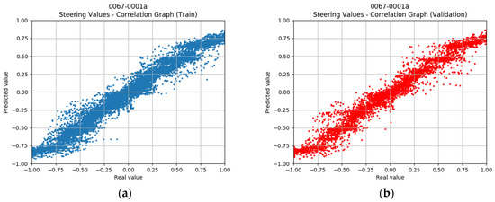
Figure 13. Correlation graphs for the expected vs. the predicted steering angle, images sized at 160 × 120, and the dataset DR1. (a) Scatter plot for the training set. (b) Scatter plot for the validation set.

In this case, the model has a slightly weaker ability to approximate the identity function. For example, for some samples, a steering value near 1.0 is expected, but the model delivers a lower value. In the physical evaluation, the driving model tends to take the curves somewhat more gently with respect to the human driver. A few more outliers can be identified with respect to the previous case. Despite achieving the worst approximation, with this model, the car drives with greater correction. The assumption is that the driving model has a certain ability to correct mistakes made in a timely manner and that the speed of inference contributes favorably to this.

A detailed review of the mistakes concluded that the driving style used in training might not be the most appropriate. As already discussed in the previous section, a new dataset was built using a more precise driving style (dataset DR2, Table 2).

The results of this experiment in this new set are satisfactory, managing to cover the complete circuit without losing track. In addition, it can be observed how the driving model imitates the original behavior, performing curve tracing with the modified technique. Figure 14 shows the correlation graphs for dataset DR2.

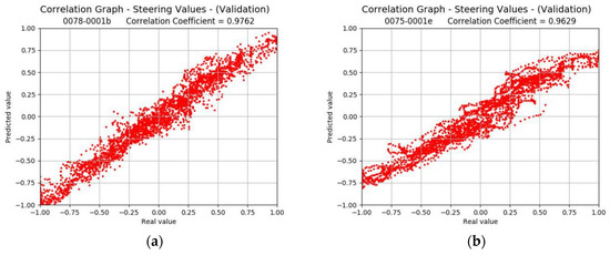
Figure 14. Correlation graphs for the expected vs. the predicted steering values for the proposed model with the dataset DR2 and only validation. (a) Scatter plot for the validation set 320 × 240. (b) Scatter plot for the validation set 160 × 120.

Although the model seems to have a slightly weaker approximation ability, which is more notable in cases when extreme steering angles are needed, the dataset facilitates a better driving performance. In physical tests, the car shows that it is able to drive correctly with smoother turns, recovering more easily from incorrect decisions, thanks to the higher rate of inference.

4.3. Comparison

To test the behavior of the trained models, dataset DR2 is used. A further evaluation is performed with the dataset DR3, which has been obtained with a modified circuit and placed in a different context. The first model is an end-to-end model, which combines a CNN to process the input images and an MLP, following proposals such as that in Reference [14]. The second model uses a first encoder combined with an MLP. The encoder is trained with the entire Autoencoder to learn the identity function, i.e., the image from the camera is used at the same time at the input and output of the Autoencoder. This approach is the same as in Reference [18]. None of these models rely on semantic segmentation, but the experiments can be performed with both the augmented datasets and without augmentation.

Figure 15 shows the corresponding correlation graphs for dataset DR3.

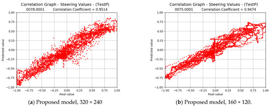
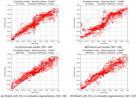
Figure 15. Correlation graphs for the proposed (a,b), the end-to-end (c,d) models, and the Autoencoder without semantic segmentation (e,f). Expected vs. predicted steering values with the dataset DR3 and only test. Training is performed with the augmented dataset.

The values of the correlation coefficients degrade slightly for the proposed model when the DR3 dataset is used. For the end-to-end model, the degradation is relatively high. This can be explained by the fact that this model can base its decisions on large amounts of information from the images, so it does not have to focus exclusively on the road lines to learn the driving task. It can make decisions based on additional and spurious elements that, in the case of the proposed model, are eliminated with semantic segmentation. Since the DR3 dataset is based on a different circuit, placed differently and with different lighting, the end-to-end model will have more trouble determining the steering angle.

Figure 16 and Figure 17 show the driving sequences for dataset DR3, comparing the performances of the proposed model and the other models (all working at 160 × 120 pixels).

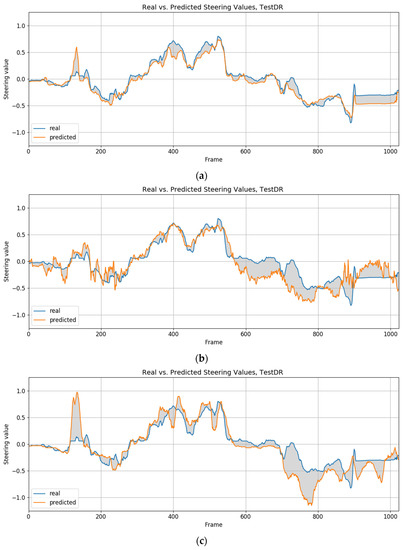
Figure 16. Comparison of the steering values provided by a human driver and the trained models, 160 × 120—driving direction right. (a) Proposed model. (b) End-to-end model. (c) Model w/o segmentation.

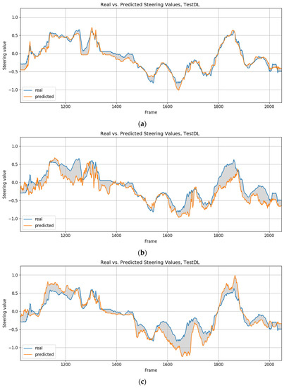
Figure 17. Comparison of the steering values provided by a human driver and the trained models, 160 × 120—driving direction left (a) Proposed model. (b) End-to-end model. (c) Model w/o segmentation.

The proposed model is relatively accurate when imitating the behavior of the human driver. The other two models that do not rely on semantic segmentation show a greater deviation from human behavior. It also makes some unexpected turning decisions. In the case of the end-to-end model, numerous spikes in the graphs indicate more erratic behavior when interpreting the images and making decisions.

The obtained correlation coefficients are summarized in Table 3.

Table 3. Correlation values for all the models, datasets, and image sizes.

Model	DR2 320 × 240	DR2 160 × 120	DR3 320 × 240	DR3 160 × 120	Dataset Augmentation
Proposed model	0.9762	0.9629	0.9514	0.9474	Yes
Proposal w/o input noise	0.9368	0.9272	0.9354	0.9079	Yes
Canny Detector + CNN	0.9798	0.9607	0.9533	0.9462	Yes
CNN w/o segmentation	0.9623	0.9542	0.9295	0.9156	Yes
AE w/o segmentation	0.9424	0.9396	0. 9151	0.9015	Yes
CNN w/o segmentation	0.9382	0.9378	0.8902	0.8823	No
AE w/o segmentation	0,9347	0.9219	0.8931	0.8745	No

Various issues can be identified. The correlation is lower when using the alternative dataset DR3. There is also a reduction when using images with a smaller size, making this a relevant aspect: getting a better performance implies the need for greater computing capacity. Using the Canny Edge Detector approach provides similar results to those of the proposed model, while the use of input noise for training the Autoencoder seems to be essential for a good performance.

Both the end-to-end model and the Autoencoder without semantic segmentation show lower correlation coefficients. They benefit greatly from the proposed dataset augmentation using image overlay. This implies that the proposed model is more efficient in this task and that image superposition achieves better results with reduced datasets.

4.4. Additional Validation Experiments

Additional validation is carried out by testing the automated driving capacity in situations that present certain complications—in particular, those containing highlights, shadows, occlusions, and illumination changes.

Based on dataset DR3 with images sized at 160 × 120, variations are generated in which image sequences are randomly modified:

(a)

segments of the images are blackened or whitened, simulating either occlusions or intense reflections.

(b)

darkening or lightening of segments or the entire image, simulating either shadows or light reflections or general changes in lighting.

The modifications (segment size and intensity) are generated randomly, with some limitations to avoid excessive image deterioration. This approach allows an evaluation of the results based on the semantic segmentation provided by the dataset. Table 4 shows the correlation coefficients for the best models from the previous experiments. The same sequence of the modified images is used for each model.

Table 4. Correlation coefficients for dataset DR3 at 160 × 120 with image modifications. Considered is the total whitening or blackening of an image section or slight lightening or darkening of a partial section or the full image. The first column contains the correlation coefficients for the original dataset.

Model	w/o Change	White	Black	Light	Dark
Proposed model	0.9474	0.9026	0.9404	0.9284	0.9431
Proposal w/o input noise	0.9079	0.7859	0.8325	0.8203	0.8402
Canny Detector + CNN	0.9462	0.8177	0.8675	0.8471	0.8684

The coefficients show certain patterns of behavior. The worst results are obtained when a section of the image turns white. This makes sense, since the key elements to detect are the white lines. In contrast, the occlusion with a black region does not pose many problems for the proposed model. Both the model based on the Canny edge detector and the model trained without input noise suffer considerably in the results. Correlation values near 0.8 represent models with either a poor approximation capability or extreme outliers.

The fact that the difference is so remarkable between the proposed model trained with noise and without noise leads us to suppose that this aspect may be fundamental to obtaining a more robust model.

A physical simulation was also carried out to determine the behavior of the Autoencoder in the indoor environment. A sample is shown in Figure 18. In most cases, the reconstruction is correct except for the affected area, and although occasionally the Autoencoder only delivers a partial reconstruction, it is usually adequate to complete the driving task.

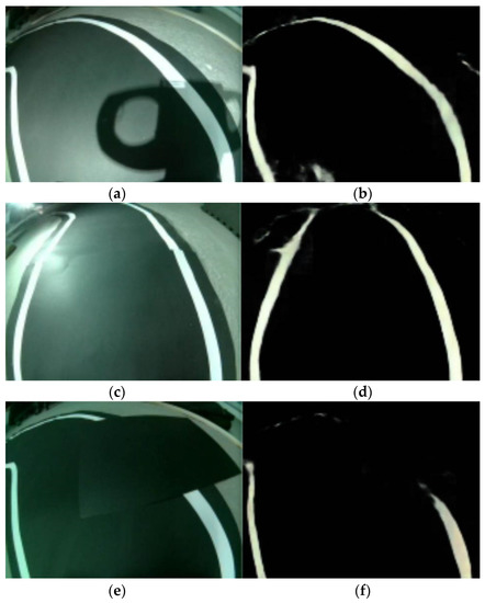
Figure 18. Different input images and output reconstruction of the Autoencoder with different difficulties: (a,b) shadow, (c,d) light reflection, and (e,f) partial occlusion.

More details are shown in the repository for this project [39]. Video 6 shows the behavior of the car when encountering different types of difficulties. A final trial is performed with a different-shaped track, shown in video 7.

5. Discussion

In this section, additional details are discussed.

There is some evidence that downsizing the image causes some loss of detail, especially in the most distant areas of the scene. This results in the worse coding or reconstruction of the relevant elements and somewhat lower correlation coefficients. However, the higher inference rate achieved compensates for this deterioration, allowing small continuous corrections to be made to the steering angle. This provides a better overall driving result.

Including the semantic segmentation phase in an end-to-end model provides several advantages. The results show that a more robust model is obtained, as it can remove redundant elements from the scene. It also provides a simple mechanism to deliver an interpretation of the scene. For a given driving scene, the full Autoencoder can be used to obtain the semantic segmentation performed by the encoder. This facilitates the detection of causes of a driving failure, which is not so easy in end-to-end models.

A further advantage of the proposed model concerns the decomposition of the learning task into two tasks: feature extraction and driving learning. The development of the system is more flexible, making it possible to approach the work incrementally and reduce the required training time. Once the Autoencoder has been trained, training the steering network is a faster process. In this way, it is possible to train different driving styles more quickly. An approach based on a single task training a convolutional neural network necessitates retraining the entire network.

The advantage of image superposition is that it allows the generation of larger datasets, by combinatorics, than those that can be obtained from plain supervised driving.

The supervised training of an autonomous driving system based on semantic segmentation has the disadvantage of requiring a dataset with accurate semantic interpretation of the scenes and their elements. As this is difficult to achieve in the real world, an initial phase of training using simulators is needed, which, in turn, has the disadvantage of lacking realism in the generated images. Our proposal has the advantage of performing the same process of semantic interpretation in an indoor environment using chroma key techniques.

6. Conclusions

A small-scale model car could be trained to perform a lane-following task.

The stage built with chromas allowed us to segment the lines of the road from the rest of the elements in the scene and correctly identify them in a single step. This replicates the advantages that usual simulators provide, avoiding either time-consuming labeling tasks or the need to combine other conventional techniques to segment and identify the elements of the image in a target scenario.

The use of augmented images made it possible to train an Autoencoder capable of replicating the segmentation without having to resort to simulators. Furthermore, a noise addition in the input data helps to generate Autoencoders with a higher tolerance to environmental and illumination variations.

In the validation tests, the driving model was found to be robust to changes in lighting on the stage, as well as to shadows or to the presence of obstacles on the track. In the presence of an occlusion on one of the lines, the driving model is able to follow the other line. In addition, it was found that the car was able to follow a different circuit than the one used for training.

The approach discussed in this project shows an interesting and alternative method to automate the training of vehicle steering without the use of driving simulators.

Tasks for future work include developing a more elaborate proposal based on a mixed reality system, using generative methods to induce variations in lighting and perspective, and including more elements (road signs, for example) in the semantic segmentation. This would allow the merging of the training process in both simulators and real environments, retaining the advantages of both.

References

- Pomerlau, D.A. ALVINN: An Autonomous Land Vehicle in a Neural Network. Adv. Neural Inf. Process. Syst. 1989, 1, 305–311. [Google Scholar]
- Williams, M. PROMETHEUS—The European research programme for optimising the road transport system in Europe. In IEEE Colloquium on Driver Information; IET: London, UK, 1988. [Google Scholar]
- Grigorescu, S.; Trasnea, B.; Cocias, T.; Macesanu, G. A survey of deep learning techniques for autonomous driving. J. Field Robot. 2019, 37, 362–386. [Google Scholar] [CrossRef]
- Liu, M.; Deng, X.; Lei, Z.; Jiang, C.; Piao, C. Autonomous Lane Keeping System: Lane Detection, Tracking and Control on Embedded System. J. Electr. Eng. Technol. 2021, 16, 569–578. [Google Scholar] [CrossRef]
- Ahn, T.; Lee, Y.; Park, K. Design of Integrated Autonomous Driving Control System that Incorporates Chassis Controllers for Improving Path Tracking Performance and Vehicle Stability. Electronics 2021, 10, 144. [Google Scholar] [CrossRef]
- Wu, Z.; Qiu, K.; Yuan, T.; Chen, H. A method to keep autonomous vehicles steadily drive based on lane detection. Int. J. Adv. Robot. Syst. 2021, 18. [Google Scholar] [CrossRef]
- Lin, Y.-C.; Lin, C.-L.; Huang, S.-T.; Kuo, C.-H. Implementation of an Autonomous Overtaking System Based on Time to Lane Crossing Estimation and Model Predictive Control. Electronics 2021, 10, 2293. [Google Scholar] [CrossRef]
- Shen, H. Complex Lane Line Detection Under Autonomous Driving. In 2020 5th International Conference on Mechanical, Control and Computer Engineering (ICMCCE); IEEE: Piscataway, NJ, USA, 2020; pp. 627–631. [Google Scholar]
- Haris, M.; Glowacz, A. Lane Line Detection Based on Object Feature Distillation. Electronics 2021, 10, 1102. [Google Scholar] [CrossRef]
- Lin, H.-Y.; Dai, J.-M.; Wu, L.-T.; Chen, L.-Q. A Vision-Based Driver Assistance System with Forward Collision and Overtaking Detection. Sensors 2020, 20, 5139. [Google Scholar] [CrossRef] [PubMed]
- Meng, Q.; Zhao, X.; Hu, C.; Sun, Z.-Y. High Velocity Lane Keeping Control Method Based on the Non-Smooth Finite-Time Control for Electric Vehicle Driven by Four Wheels Independently. Electronics 2021, 10, 760. [Google Scholar] [CrossRef]
- Sun, C.; Vianney, M.U.; Cao, D. Affordance Learning In Direct Perception for Autonomous Driving. 2019. Available online: https://arxiv.org/abs/1903.08746 (accessed on 10 December 2021).
- Maanpää, J.; Taher, J.; Manninen, P.; Pakola, L.; Melekhov, J.; Hyyppä, J. Multimodal End-to-End Learning for Autonomous Steering in Adverse Road and Weather Condition. In Proceedings of the 25th International Conference on Pattern Recognition (ICPR), Milan, Italy, 10–15 January 2021. [Google Scholar]
- Bojarski, M.; Del Testa, D.; Dworakowski, D.; Firner, B.; Flepp, B.; Goyal, P.; Jackel, L.D.; Monfort, M.; Muller, U.; Zhang, J.; et al. End to End Learning for Self-Driving Cars. arXiv 2016, arXiv:1604.07316. Available online: http://arxiv.org/abs/1604.07316 (accessed on 10 December 2021).
- Toromanoff, M.; Wirbel, E.; Wilhelm, F.; Vejarano, C.; Perrotton, X.; Moutarde, F. End to end vehicle lateral control using a single fisheye camera. In Proceedings of the IEEE/RSJ International Conference on Intelligent Robots and Systems (IROS), Madrid, Spain, 1–5 October 2018. [Google Scholar]
- Codevilla, F.; Müller, M.; Lopez, A.; Koltun, V.; Dosovitskiy, A. End-to-end driving via conditional imitation learning. In Proceedings of the IEEE International Conference on Robotics and Automation (ICRA), Brisbane, QLD, Australia, 21–25 May 2018. [Google Scholar]
- Mehta, A.; Subramanian, A.; Subramanian, A. Learning end-to-end autonomous driving using guided auxiliary supervision. arXiv 2018, arXiv:1808.10393. Available online: https://arxiv.org/abs/1808.10393 (accessed on 10 December 2021).
- Yang, Y.; Wu, Z.; Xu, Q.; Yan, F. Deep Learning Technique-Based Steering of Autonomous Car. Int. J. Comput. Intell. Appl. 2018, 17, 1850006. [Google Scholar] [CrossRef]
- Cordts, M.; Omran, M.; Ramos, S.; Rehfeld, T.; Enzweiler, M.; Benenson, R.; Franke, U.; Roth, S.; Schiele, B. The Cityscapes Dataset for Semantic Urban Scene Understanding. In Proceedings of the IEEE Conference on Computer Vision and Pattern Recognition (CVPR), Las Vegas, NV, USA, 26 June–1 July 2016; pp. 3213–3223. [Google Scholar]
- Codevilla, F.; Santana, E.; Lopez, A.M.; Gaidon, A. Exploring the limitations of behavior cloning for autonomous driving. In Proceedings of the IEEE/CVF International Conference on Computer Vision, Seoul, Korea, 27–28 October 2019. [Google Scholar]
- Rumelhart, D.E.; Hinton, G.; Williams, R.J. Learning Internal Representations by Error Propagation. In Explorations in the Microstructure of Cognition; MIT Press: Cambridge, MA, USA, 1986; Volume 1, pp. 318–362. [Google Scholar]
- Alonso-Weber, J.M.; Sesmero, M.P.; Sanchis, A. Combining additive input noise annealing and pattern transformations for improved handwritten character recognition. Expert Syst. Appl. 2014, 41, 8180–8188. [Google Scholar] [CrossRef]
- Sietsma, J.; Dow, R.J.F. Creating artificial neural networks that generalize. Neural Netw. 1991, 4, 67–79. [Google Scholar] [CrossRef]
- Vincent, P.; Larochelle, H.; Bengio, Y.; Manzagol, P.-A. Extracting and composing robust features with denoising autoencoders. In Proceedings of the 25th international conference on Machine learning-ICML, Helsinki, Finland, 5–9 July 2008; pp. 1096–1103. [Google Scholar]
- Vincent, P.; Larochelle, H.; Lajoie, I.; Yoshua, B.; Manzagol, P.-A. Stacked Denoising Autoencoders: Learning Useful Representations in a Deep Network with a Local Denoising Criterion. J. Mach. Learn. Res. 2010, 11, 3371–3408. [Google Scholar]
- Badrinarayanan, V.; Kendall, A.; Cipolla, R. SegNet: A Deep Convolutional Encoder-Decoder Architecture for Image Segmentation. IEEE Trans. Pattern Anal. Mach. Intell. 2017, 39, 2481–2495. [Google Scholar] [CrossRef] [PubMed]
- Yamashita, A.; Agata, H.; Kaneko, T. Every color chromakey. In Proceedings of the 19th International Conference on Pattern Recognition, Tampa, FL, USA, 8–11 December 2008; pp. 1–4. [Google Scholar]
- Sharma, R.; Deora, R.; Vishvakarma, A. AlphaNet: An Attention Guided Deep Network for Automatic Image Matting. In Proceedings of the 2020 International Conference on Omni-layer Intelligent Systems (COINS), Virtual Online, 31 August–2 September 2020; pp. 1–8. [Google Scholar]
- Varatharasan, V.; Shin, H.-S.; Tsourdos, A.; Colosimo, N. Improving Learning Effectiveness for Object Detection and Classification in Cluttered Backgrounds. In Proceedings of the 2019 Workshop on Research, Education and Development of Unmanned Aerial Systems (RED UAS), Cranfield, UK, 25–27 November 2019; pp. 78–85. [Google Scholar]
- Nguyen, T.; Miller, I.D.; Cohen, A.; Thakur, D.; Guru, A.; Prasad, S.; Taylor, C.J.; Chaudhari, P.; Kumar, V. PennSyn2Real: Training Object Recognition Models Without Human Labeling. IEEE Robot. Autom. Lett. 2021, 6, 5032–5039. [Google Scholar] [CrossRef]
- Rangesh, A.; Trivedi, M.M. HandyNet: A One-stop Solution to Detect, Segment, Localize & Analyze Driver Hands. In Proceedings of the 2018 IEEE/CVF Conference on Computer Vision and Pattern Recognition Workshops (CVPRW), Salt Lake City, UT, USA, 18–22 June 2018; pp. 1103–1110. [Google Scholar]
- Hearn, D.D.; Baker, M.P. Computer Graphics with OpenGL, 2; Pearson: Boston, MA, USA, 2011. [Google Scholar]
- Yurtsever, E.; Lambert, J.; Carballo, A.; Takeda, K. A Survey of Autonomous Driving: Common Practices and Emerging Technologies. IEEE Access 2020, 8, 58443–58469. [Google Scholar] [CrossRef]
- Tampuu, A.; Matiisen, T.; Semikin, M.; Fishman, D.; Muhammad, N. A Survey of End-to-End Driving: Architectures and Training Methods; IEEE: Piscataway, NJ, USA, 2020; pp. 1–21. [Google Scholar]
- Kuzmic, J.; Rudolph, G. Comparison between Filtered Canny Edge Detector and Convolutional Neural Network for Real Time Lane Detection in a Unity 3D Simulator. In Proceedings of the 6th International Conference on Internet of Things, Big Data and Security, Prague, Czech Republic, 23–25 April 2021; pp. 148–155. [Google Scholar]
- OpenCV. Available online: https://opencv.org/ (accessed on 10 December 2021).
- Franke, C. Autonomous Driving with a Simulation Trained Convolutional Neural Network. Ph.D. Thesis, University of the Pacific, Stockton, CA, USA, 2017. [Google Scholar]
- Repository for This Project. Available online: https://github.com/javiercorrochano/PaperAutonomousCar (accessed on 10 December 2021).
- Masci, J.; Meier, U.; Cireşan, D.; Schmidhuber, J. Stacked Convolutional Auto-Encoders for Hierarchical Feature Extraction. Artif. Neural Netw. Mach. Learn. 2011, 6791, 52–59. [Google Scholar]
Publisher’s Note: MDPI stays neutral with regard to jurisdictional claims in published maps and institutional affiliations. |
© 2021 by the authors. Licensee MDPI, Basel, Switzerland. This article is an open access article distributed under the terms and conditions of the Creative Commons Attribution (CC BY) license (https://creativecommons.org/licenses/by/4.0/).