Rollover Prevention Control for Autonomous Electric Road Sweeper

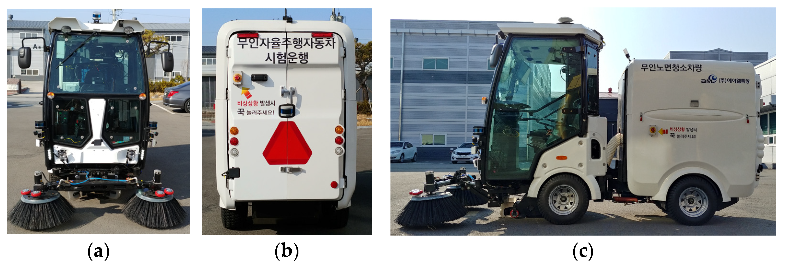
Abstract

This paper presents a method to prevent the rollover of autonomous electric road sweepers (AERS). AERS have an articulated frame steering (AFS) mechanism. Moreover, the heights of the center of gravity of the front and rear bodies are high. As such, they are prone to rolling over at low speeds and at small articulation angles. A bicycle model with a nonlinear tire model was used as a vehicle model for AERS. Using that vehicle model, path tracking and speed controllers were designed in order to follow a predefined path and speed profile, respectively. To check the rollover propensity of AERS, load transfer ratio (LTR) based the rollover analysis was completed. Based on the results of the analysis, a rollover prevention scheme was proposed. To validate the proposed scheme, a simulation was conducted using a U-shaped path under constant speed conditions. From the simulation, it was shown that the proposed scheme is effective in preventing AERS from rolling over.

1. Introduction

Road sweepers are used to clean urban roadsides. They originated in the17th century. Their power source has changed over time, starting from a horse before eventually moving to being powered by an internal combustion engine and finally, to an electric motor. The current road sweepers that are being used today were developed in the 1950s [1]. The details of various sweeping machines with different operating requirements have been classified in SAE standard, J2130 [2]. A history of road cleaning vehicles is summarized in [3].

The recent advances in road sweeper developments can be categorized into two aspects: The first is an electrification, which was developed in order to cope with environmental issues [4,5,6]. Up until the 2000s, most road sweepers used a diesel engine as their power source, which resulted in the creation of air pollution due to emissions of compounds such as NOx and particulate matter [7]. To cope with this problem, the diesel engine in road sweepers was replaced with an electric motor and a battery. The second is autonomous driving, which we developed in order to maximize utilization in dedicated areas such as airports or public parks without a human driver [8,9,10]. For example, most passenger vehicles are utilized within 20% of their total lifecycle. On the contrary, autonomous road sweepers can be utilized by up to 90% because there are no human drivers [11]. Moreover, they can be operated from late night to dawn by virtue of autonomous driving. Another purpose of autonomous driving for road sweepers is to protect sanitation workers from injury caused by traffic accidents and to free them from heavy physical labor. This type of vehicle is referred to as an autonomous electric road sweeper (AERS).

Following these trends, several AERSs have been produced so far. A typical example is “Donner”, which is developed by a consortium led by Bucher Municipal and ENWAY [12]. This vehicle is based on Bucher Municipal’s fully electric vehicle (EV), CityCat 2020 ev. Moreover, it passed the Land Transport Authority’s approval test for autonomous vehicles for use on public roads. In 2021, Singapore’s National Environment Agency (NEA) began trial runs using autonomous road sweepers on public roads [13]. Boschung has also created an AERS called the Urban-Sweeper S2.0 [14]. Figure 1 shows the AERS that has recently been developed by the Korea Institute of Industrial Technologies (KIIT) in 2019 and the AM Special Vehicle (AMSV) [15]. This is quite similar to Boschung’ AERS.

Figure 1. Autonomous electric road sweeper considered in this paper. (a) Front view; (b) Rear view; (c) Side view.

Generally, a small-sized road sweeper, such as the one seen in Figure 1, has articulated frame steering (AFS) as a steering mechanism [16,17]. Figure 2 shows the structure of AFS. As shown in Figure 2, the vehicle consists of the front and rear bodies. In Figure 1, θ is the articulation angle at the center joint. In this type of vehicle, steering is achieved by changing the articulation angle using the hydraulic cylinder between the front and rear bodies. This type of steering has generally been adopted in construction machines such as wheel loaders, scrapers, loaders, and skidders [18,19]. Boschung’s Urban-Sweeper S2.0 as well as the KIIT and AMSV’s AERS have this type of a steering mechanism as well, i.e., AFS. By virtue of its structure, a vehicle with AFS has excellent maneuverability, i.e., agility, which can provide a faster yaw rate with respect to an identical steering angle. Moreover, it can provide a smaller turning radius on a single lane road [16]. However, this means that larger lateral acceleration can be generated by a smaller steering angle compared to front-wheel-steered vehicles. Another drawback of AFS is the snaking instability phenomenon that occurs at high speeds [18].

Figure 2. Structure of articulated frame steering.

For autonomous driving, several functions are needed. These functions include localization, path generation and tracking control, speed control, obstacle detection and avoidance, and autonomous parking [20,21]. In view of control, path tracking and speed controls are the most important aspects [8]. Path tracking control means that the driver model, which generates the steering angle command, needs to follow a given path [9,10,21,22,23]. The speed control ensures that the vehicle follows a given speed profile by means of engine throttle or motor torque commands [8,9]. The pure pursuit method is implemented as the patch tracking controller in AERS, as shown in Figure 1. The speed controller is designed with a sliding mode control and is implemented into AERS, as shown in Figure 1.

The AERS shown in Figure 1 has special features. The first is low speed. The maximum and operational speeds of this vehicle are 20 km/h and 5 km/h, respectively [8]. As such, there have been few issues in terms of lateral stability or yaw moment control, which are needed to stabilize the snaking phenomenon that is inherent in vehicles with AFS [16]. Moreover, this vehicle has rear-wheel drive with a single motor and a pneumatic braking system without an independent braking function. In other words, this vehicle has no differential braking or torque vectoring functions [18,19]. As such, it is impossible for one to apply yaw moment control with differential braking or torque vectoring in this vehicle. The second is that this vehicle has an AFS mechanism. By virtue of AFS, this vehicle has excellent maneuverability [16]. In other words, the turning radius is smaller, and the yaw rate is larger than that of front-wheel-steered vehicles under an identical steering angle. This means that the lateral acceleration generated by steering is larger in this vehicle. The third is that the tread is quite small, and the height of center of gravity (CoG) is quite high. Moreover, the rear body of the ARES has no suspension. This is because the AERS is an autonomous vehicle that can drive without a driver. As such, an active suspension used for ride comfort enhancement is not needed. As a result, this vehicle is easily prone to rolling over, even at low speeds. Because of this, it is necessary to analyze the rollover propensity of this vehicle and to design a controller to prevent rollover.

To analyze the rollover propensity of this vehicle, a simulation with open-loop steering, i.e., J-turn maneuver, was conducted. The rollover measure was the load transfer ratio (LTR), which was defined as the ratio between the vertical forces of the left and right wheels [24]. From the analysis, the lateral acceleration and LTR corresponding to rollover were identified. With those values, the activation condition of the rollover prevention controller was defined, and the reference speed needed to prevent rollover was calculated.

To prevent the AERS from rolling over, a rollover prevention scheme is proposed in this paper. To date, several rollover prevention controls or schemes have been proposed for passenger or commercial heavy vehicles [24,25,26,27,28,29,30]. In the literature, differential braking, active steering, active suspension, and torque vectoring devices have been adopted as actuators for rollover prevention. However, all of the the actuators used in previous research cannot be used for rollover prevention because the AERS only has rear-wheel drive with a single motor. On the other hand, recent research has investigated both the rollover prevention and path tracking controls simultaneously [27,28,29]. For the AERS, the path tracking controller is needed to follow a pre-defined path. In other words, steering cannot be used for rollover prevention purposes. For the reason, only the speed controller is available for rollover prevention in the AERS. As such, the rollover prevention scheme proposed in this paper intends to generate a reference speed profile that can be used for rollover prevention.

In this paper, the AERS is modeled with a bicycle model that comprises the front and rear bodies. The Dugoff tire model is adopted as a nonlinear tire model. With the parameters obtained from the real AERS, the vehicle model is validated through the comparison between the simulation and the experimental data. Figure 3 shows the schematic diagram of the AERS control system. As shown in Figure 3, a pure pursuit method is adopted as a driver model in the path tracking controller. A speed controller is designed with the vehicle model using sliding mode control. For rollover prevention, two schemes that are needed to generate the reference speed profile are proposed. With the rollover prevention schemes, the methods are applied as the reference speed generator in Figure 3. To check the rollover propensity of the AERS and to show the effectiveness of the proposed rollover prevention scheme, a simulation is conducted in the MATLAB/Simulink environment.

Figure 3. Schematic diagram of AERS control system.

This paper consists of four sections. In Section 2, the vehicle model for the road sweeper is built and the motion equations are derived. LTR is defined as the rollover index. The steering and speed controllers are designed in Section 3. With those controllers, the rollover prevention scheme is proposed. In Section 4, rollover propensity analysis is conducted, and the simulation is conducted to show the effectiveness of the proposed rollover prevention scheme. In the last section, Section 5, the conclusion of this research is given.

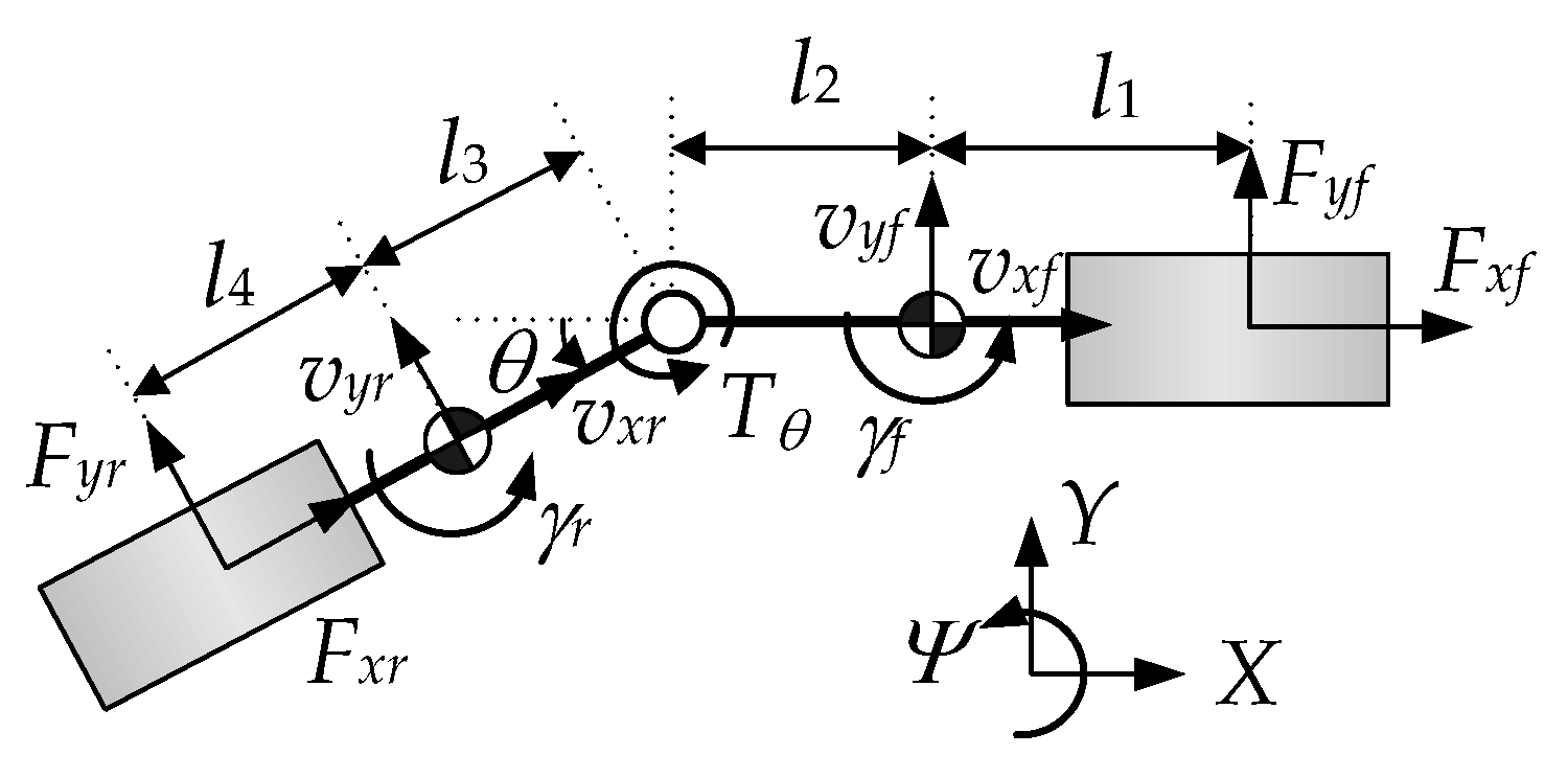
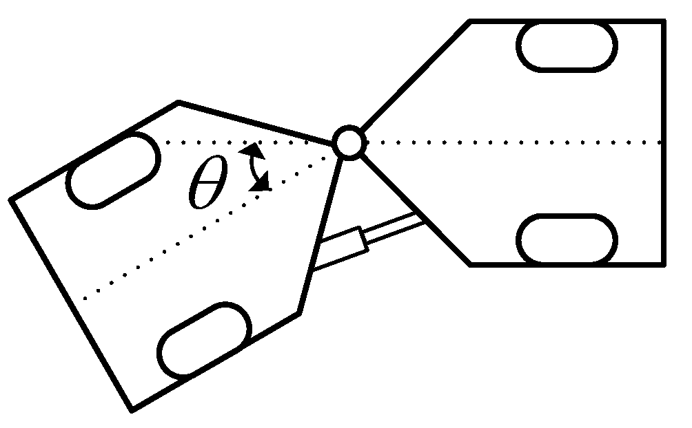
2. Modeling of Vehicle with Articulated Frame Steering

2.1. Vehicle Modeling

As described in the explanation in Figure 1, the AERS has a single motor connected to the rear wheels and a pneumatic braking system without an independent braking function. As a result, the AERS has no differential braking or torque vectoring function. As such, it is not necessary to separate the left and right wheels in a vehicle model. For this reason, the AERS is modeled with a bicycle model in this paper. Figure 4 shows the free-body diagram of the bicycle model for the AERS [9,25,26]. As shown in Figure 4, the vehicle model consists of the front and rear bides. Because of this, the acceleration, the velocity, and the yaw rate are defined on the front and rear bides. Explanations on all of the symbols in Figure 4 are given in the Nomenclature section at the end of the paper.

Figure 4. Free body diagram of the bicycle model for AERS.

Generally, motion equations are derived with respect to the front body when modeling a vehicle with AFS. The rotational motion equations for the front and rear bodies are derived as Equation (1). These equations are derived from the moment equilibrium around the CoGs of the front and rear bodies. In Equation (1), T_θ is the moment generated by a hydraulic cylinder between the front and rear bodies. By virtue of T_θ, the articulation angle θ is generated. R(θ) given in Equation (2) is the rotation matrix with the articulation angle. With the rotation matrix, the equations for the longitudinal and lateral motions of the front and rear bodies are derived as Equation (3). In Equation (3), the longitudinal and lateral accelerations of the front and rear bodies are defined as Equation (4). From the yaw rate of the front body and the articulation angular rate, the yaw rate of the rear body is defined as Equation (5). With the rotation matrix and Equation (5), the longitudinal and lateral velocities of the rear body are calculated from those of the front body, as given in Equation (6). A detailed derivation procedure from Equation (1) to Equation (6) can be found in the references [9,16,31].

$$\{\begin{array}{l}{I}_{zf}{\dot{\gamma }}_f=F_{yf}\left(l_1+l_2\right)-l_2{m}_f{a}_{yf}+T_{\theta }\\ I_{zr}{\dot{\gamma }}_r=-F_{yr}\left(l_3+l_4\right)+l_3{m}_r{a}_{yr}-T_{\theta }\end{array}$$

(1)

$$R\left(\theta \right)=\left[\begin{array}{cc}\cos \theta & -\sin \theta \\ \sin \theta & \cos \theta \end{array}\right]$$

(2)

$$\left[\begin{array}{c}{F}_{xf}-m_f{a}_{xf}\\ F_{yf}-m_f{a}_{yf}\end{array}\right]+R\left(\theta \right)\left[\begin{array}{c}{F}_{xr}-m_r{a}_{xr}\\ F_{yr}-m_r{a}_{yr}\end{array}\right]=0$$

(3)

$$\{\begin{array}{l}{a}_{xf}={\dot{v}}_{xf}-v_{yf}{\gamma }_f\hspace{1em}\\ a_{yf}={\dot{v}}_{yf}+v_{xf}{\gamma }_f\end{array}\hspace{1em}\hspace{1em}\{\begin{array}{l}{a}_{xr}={\dot{v}}_{xr}-v_{yr}{\gamma }_r\hspace{1em}\\ a_{yr}={\dot{v}}_{yr}+v_{xr}{\gamma }_r\end{array}$$

(4)

$${\gamma }_r={\gamma }_f+\dot{\theta }$$

(5)

$$\left[\begin{array}{c}{v}_{xr}\\ v_{yr}\end{array}\right]=R\left(-\theta \right)\left[\begin{array}{c}{v}_{xf}\\ v_{yf}-l_2{\gamma }_f\end{array}\right]-\left[\begin{array}{c}0\\ l_3{\gamma }_r\end{array}\right]$$

(6)

The rotational motion equations for the front and rear wheels are given in Equation (7). In Equation (7), T_f and T_r are the traction/braking torques applied to the front and rear wheels, respectively. The AERS considered in this paper has a rear-wheel drive. As such, T_f is always set to zero, and Tr is used as a control input.

$$I_{wi}{\omega }_i=T_i-r_{wi}{F}_{xi},\hspace{1em}i=f,r$$

(7)

To calculate a tire force using a mathematical model, it is necessary to calculate the slip ratio and slip angle with the dynamic variables that were obtained from the equations for the motion of the vehicle bodies and wheels. The slip ratio λ is defined as the ratio between the rotational and translational speeds of a wheel, calculated as Equation (8) [9,16]. The slip angle α is defined as the angle between the steering and wheel travel directions, as calculated in Equation (9) [9,16]. To calculate the longitudinal and lateral tire forces in Equations (1), (3), and (7), the Dugoff tire model is adopted in this paper [16]. From the Dugoff model, the longitudinal and lateral tire forces are calculated as Equation (10). In Equation (10), the quantities S_i and f(S_i) are calculated as Equation (11). In Equations (10) and (11), C_x and C_y are the longitudinal and lateral cornering stiffness of the tire, respectively. These values were derived from experimental data on a particular tire.

$${\lambda }_i=\{\begin{array}{l}\frac{r_{wi}{\omega }_i-v_{xi}}{r_{wi}{\omega }_i},\hspace{1em}{r}_{wi}{\omega }_i>v_{xi}\\ \frac{r_{wi}{\omega }_i-v_{xi}}{v_{xi}},\hspace{1em}{r}_{wi}{\omega }_i<v_{xi}\end{array}\hspace{1em}i=f,r$$

(8)

$${\alpha }_i={\tan }^{-1}\left(\frac{v_{yi}}{v_{xi}}\right),\hspace{1em}i=f,r$$

(9)

$$F_{xi}=C_x\frac{{\lambda }_i}{1-{\lambda }_i}f\left(S_i\right),\hspace{1em}{F}_{yi}=C_y\frac{\tan {\alpha }_i}{1-{\lambda }_i}f\left(S_i\right),\hspace{1em}i=f,r$$

(10)

$$f\left(S_i\right)=\{\begin{array}{l}{S}_i\left(2-S_i\right)\hspace{0.17em}\hspace{0.17em}if\hspace{0.17em}\hspace{0.17em}\hspace{0.17em}{S}_i<1\\ 1\hspace{1em}\hspace{1em}\hspace{1em}\hspace{0.17em}\hspace{0.17em}\hspace{0.17em}if\hspace{0.17em}\hspace{0.17em}\hspace{0.17em}{S}_i\ge 1\end{array},\hspace{1em}{S}_i=\frac{\mu F_{zi}\hspace{0.17em}\left(1-{\lambda }_i\right)}{2\sqrt{C_x^2{\lambda }_i^2+C_y^2{\tan }^2{\alpha }_i}},\hspace{1em}i=f,r$$

(11)

The torque T_θ generated by the hydraulic cylinder is modeled as Equation (12). In Equation (12), K_θ and C_θ are the torsional stiffness and torsional damping coefficient, respectively.

$$T_{\theta }=K_{\theta }\theta +C_{\theta }\dot{\theta }+U_{\theta }$$

(12)

The state vector is defined as Equation (13). The control inputs in this model are the traction/braking torque T_r and the input steering torque U_θ. With the definition of the state vector and the motion equations, Equations (1), (3), (7) and (12), the state-space equation for the bicycle model can be obtained as Equation (14) [9]. Two matrices in Equation (14), F(x) and G(x), are given in Equation (15) and Equation (16), respectively.

$$x={\left[\begin{array}{ccccccc}{v}_{xf}& v_{yf}& {\gamma }_f& \theta & \dot{\theta }& {\omega }_f& {\omega }_r\end{array}\right]}^T$$

(13)

$$F\left(x\right)\dot{x}=G\left(x\right)$$

(14)

$$F\left(x\right)=\left[\begin{array}{ccccccc}0& m_f{l}_2& I_{zf}& 0& 0& 0& 0\\ m_r{l}_3\sin \theta & -m_r{l}_3\cos \theta & m_r{l}_3^2+m_r{l}_2{l}_3\cos \theta +I_{zr}& 0& m_r{l}_3^2+I_{zr}& 0& 0\\ m& 0& m_r{l}_3\sin \theta & 0& m_r{l}_3\sin \theta & 0& 0\\ 0& 0& 0& 1& 0& 0& 0\\ 0& m& m_r\left(l_2+l_3\cos \theta \right)& 0& -m_r{l}_3\cos \theta & 0& 0\\ 0& 0& 0& 0& 0& I_{\omega f}& 0\\ 0& 0& 0& 0& 0& 0& I_{\omega r}\end{array}\right]$$

(15)

$$G\left(x\right)=\left[\begin{array}{c}{F}_{yf}\left(l_1+l_2\right)-m_f{l}_2{v}_{xf}{\gamma }_f+K_{\theta }\theta +C_{\theta }\dot{\theta }+U_{\theta }\\ m_r{l}_3{v}_{xf}{\gamma }_f\cos \theta +m_r{l}_3{v}_{yf}{\gamma }_f\sin \theta -m_r{l}_2{l}_3{\gamma }_f^2\sin \theta -F_{yr}\left(l_3+l_4\right)-K_{\theta }\theta -C_{\theta }\dot{\theta }-U_{\theta }\\ F_{xf}+m{v}_{yf}{\gamma }_f+F_{xr}\cos \theta -F_{yr}\sin \theta -m_r{l}_3{\gamma }_r^2\cos \theta -m_r{l}_2{\gamma }_f^2\\ \dot{\theta }\\ F_{yf}-m{v}_{xf}{\gamma }_f+F_{xr}\sin \theta +F_{yr}\cos \theta -m_r{l}_3{\gamma }_r^2\sin \theta \\ -r_{wf}{F}_{xf}\\ T_r-r_{wr}{F}_{xr}\end{array}\right]$$

(16)

As shown in Figure 1, the CoGs of the front and rear bodies on the AERS are located on the front and rear axles, respectively. As such, the parameters l₁ and l₄ are set to zero. The maximum speed and articulation angle of the real AERS as given in Figure 1 are 20 km/h and 30°, respectively.

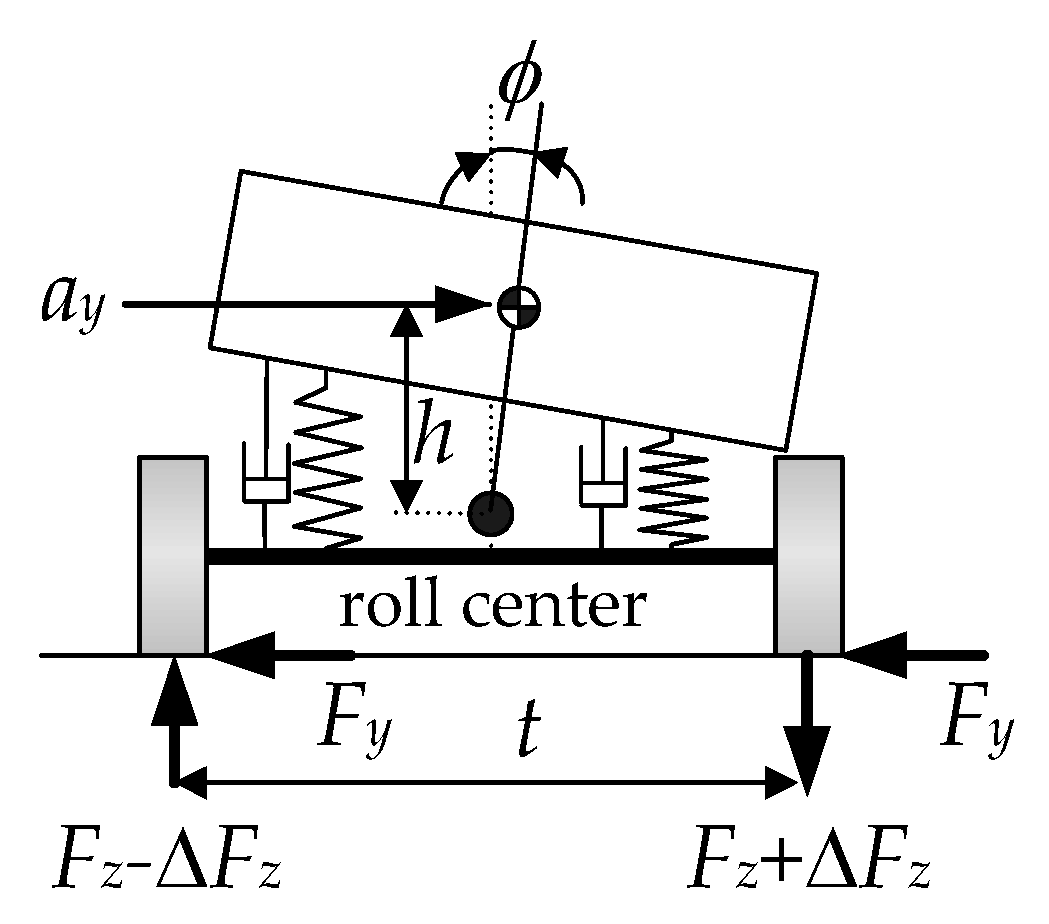
2.2. Load Transfer Ratio (LTR)

Generally, the roll motion of a vehicle is caused by the lateral acceleration, which is generated by cornering. Figure 5 shows the roll motion of a sprung mass caused by the lateral acceleration a_y, which is calculated using Equation (4). In Figure 5, h is the height of the mass center from the roll equation, and t is the track width. The roll center of the rear body of the AERS is located on the axle because it has no suspension. As such, the height of the mass center of the rear body is larger than that of the front body. The lateral acceleration causes lateral load transfer, which is represented by the vertical force variations, F_z − ∆F_z and F_z + ∆F_z, as shown in Figure 5. The larger the lateral acceleration and the height of the mass center, the smaller the track width, and the larger the lateral load transfer. The rollover condition is defined when the vertical tire force of a wheel becomes zero, which means that the wheel loses its contact on the ground.

Figure 5. Roll motion of a sprung mass caused by lateral acceleration.

There have been several indices that have been proposed to measure the rollover propensity of a vehicle [32]. These indices can be classified into two categories: static and dynamic indices. The typical static rollover index is the static stability factor (SSF), which is defined as t/2h, as given Figure 5. Among the dynamic rollover indices, the simplest one is the load transfer ratio (LTR), which reflects the lateral load transfer [30,32]. In this paper, the LTR is adopted as a rollover index.

The LTR is the ratio between the vertical tire forces of the left and right wheels [24,30,32]. As such, it is necessary to calculate the vertical tire forces caused by lateral load transfer. Neglecting longitudinal acceleration, the vertical tire forces caused by the lateral load transfer are calculated as Equation (17) [33]. In Equation (17), h_f and h_r are the heights of the mass center from the roll center of the front and rear bodies, respectively. As mentioned earlier, h_r is larger than h_f. With the vertical tire forces, the LTRs of the front and rear bodies are calculated as Equation (18) [24,30]. From Equation (18), there are no vertical tire forces if LTR is larger than or equal to 1. For instance, the vertical force of the left wheel in Figure 5 becomes zero. This condition indicates vehicle rolls over. Rollover occurs on high friction roads. On low friction roads, the lateral tire forces, F_y in Figure 5, are small. As a result, the vehicle slides in a lateral direction instead of rolling over. For this reason, LTR defined in Equation (18), which is valid only on high friction roads.

$$\begin{array}{l}{F}_{zf,left}=\frac{m_{f}g}{2}-\frac{m_f{h}_f}{t_f}{a}_{yf},\hspace{1em}{F}_{zf,right}=\frac{m_{f}g}{2}+\frac{m_f{h}_f}{t_f}{a}_{yf}\\ F_{zr,left}=\frac{m_{r}g}{2}-\frac{m_r{h}_r}{t_r}{a}_{yr},\hspace{1em}\hspace{0.17em}\hspace{0.17em}{F}_{zr,right}=\frac{m_{r}g}{2}+\frac{m_r{h}_r}{t_r}{a}_{yr}\end{array}$$

(17)

$${\mathrm{LTR}}_i=\frac{\left|F_{zi,left}-F_{zi,right}\right|}{F_{zi,left}+F_{zi,right}},\hspace{1em}i=f,r$$

(18)

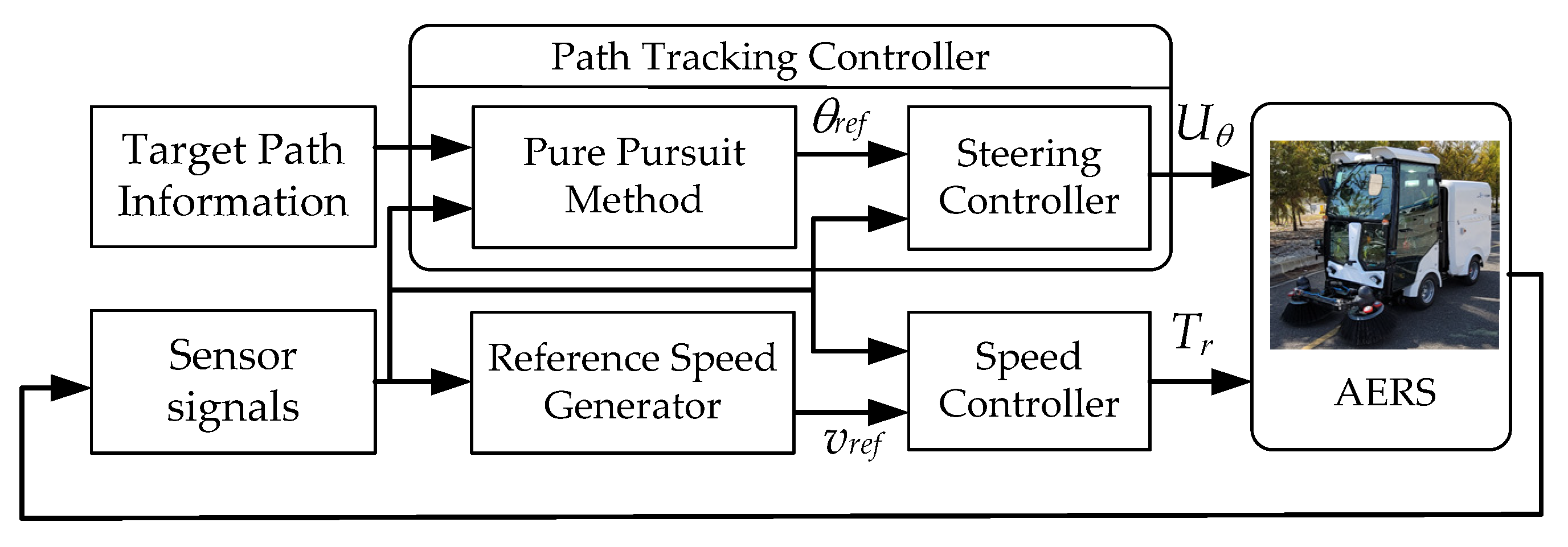
3. Controller Design

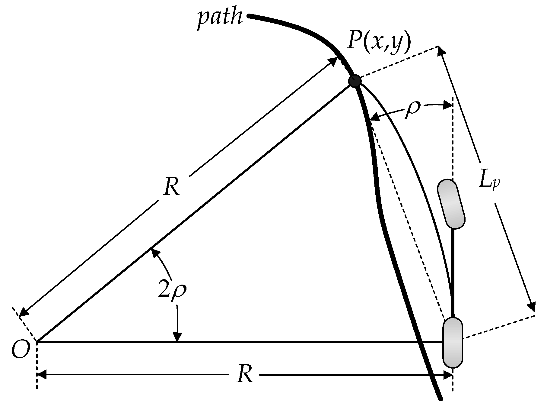
3.1. Pure Pursuit Metehod for Path Tracking Control

In this paper, a pure pursuit method is adopted to generate the articulation angle of the AERS. Figure 6 shows the geometry for the pure pursuit method [34]. In Figure 6, P(x,y) is the target point, and ρ is the angle between the vehicle’s heading vector and the look-ahead one. L_p and R are the look-ahead distance and the radius of the circular arc, respectively. In the pure pursuit method, the steering angle or the articulation angle is only determined with P(x,y) and ρ. From Figure 6, the curvature κ of the circular arc connecting P(x,y) and the rear wheel is calculated as Equation (19). With the definition of κ, the reference articulation angle is calculated as Equation (20) [34]. In Equation (20), L is the wheelbase, i.e., the distance between the front and rear axles. This articulation angle is fed into the steering controller.

$$\kappa =\frac{2\sin \rho }{L_p}$$

(19)

$${\theta }_{ref}={\tan }^{-1}\left(\kappa L\right)={\tan }^{-1}\left(\frac{2L\sin \rho }{L_p}\right)$$

(20)

Figure 6. Pure pursuit geometry.

3.2. Design of Steering and Speed Controllers

If the reference steering angle, θ_ref, is given, a controller is needed to make the articulation angle, θ, follow θ_ref. The PID controller, as given in Equation (21), is adopted in this paper.

$$U_{\theta }=K_{ps}{e}_{\theta }+K_{is}{\displaystyle \int e_{\theta }dt}+K_{ds}{\dot{e}}_{\theta },\hspace{1em}{e}_{\theta }={\theta }_{ref}-\theta$$

(21)

The speed controller is only applied to the front body. If the reference speed, v_x,ref, is given, a controller is needed to make the front body speed, v_xf, follow v_x,ref. A sliding mode control is adopted to design the speed controller in this paper [26]. From Figure 2, the equation of the longitudinal motion is obtained as Equation (22). The error surface s is defined as Equation (23). To make the error surface zero, the convergence condition (24) should be satisfied. Equation (24) represents the condition that makes the scalar variable s converge to zero as time goes to infinity. By combining Equations (22)–(24), the longitudinal force ∆F_x is obtained as Equation (25). The stability of the speed controller Equation (25) is guaranteed by Equation (24) because it is designed in such a way that Equation (24) is satisfied. The traction/braking torque applied on the rear wheel is obtained as Equation (26).

$$m\left({\dot{v}}_{xf}-v_{yf}{\gamma }_f\right)=F_{xf}+F_{xr}\cos \theta +\Delta F_x$$

(22)

$$s=v_{x,ref}-v_{xf}$$

(23)

$$\dot{s}=-K_{v}s\hspace{1em}\left(K_v>0\right)$$

(24)

$$\Delta F_x=m{\dot{v}}_{x,ref}-F_{xr}-F_{xf}-m{v}_{xf}{\gamma }_f+m{K}_v\left(v_{x,ref}-v_{xf}\right)$$

(25)

$$T_r=\frac{\Delta F_x}{r_{wr}}$$

(26)

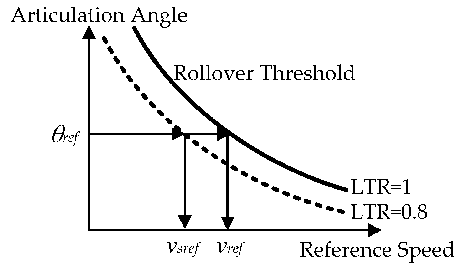
3.3. Rollover Prevention Scheme

In this paper, the intention of the proposed rollover prevention scheme is to generate a reference or desired speed that is needed to prevent the rollover. Two methods are considered when generating the reference speed.

The first method uses the definition of the lateral acceleration, as given in Equation (4). From Equation (4), the two relationships are obtained as Equation (27) [26]. The first equation of Equation (27) is obtained from Equation (4) by replacing the lateral acceleration with the desired one, a_yi,desired. In Equation (27), a_yi,desired is the lateral acceleration, which is set by a control designer. The second equation of Equation (27) is obtained from Equation (4) by replacing the lateral acceleration and the longitudinal velocity with a_yi,desired and v_xi,desired, respectively. In Equation (27), v_xi,desired is the reference speed that is needed to make the lateral acceleration be a_yi,desired for rollover prevention. By eliminating the time derivative of v_yi from the two equations of Equation (27), the desired longitudinal velocity is obtained as Equation (28). As shown in Equation (28), v_xi,desired depends on the lateral accelerations, the longitudinal velocity, and the yaw rate, regardless of the various road conditions.

$$\{\begin{array}{l}{\dot{v}}_{yi}=a_{y,measured}-v_{xi}{\gamma }_i\\ a_{yi,desired}={\dot{v}}_{yi}+v_{xi,desired}{\gamma }_i\end{array},\hspace{1em}i=f,r$$

(27)

$$v_{xi,desired}=\frac{1}{{\gamma }_i}\left\{a_{yi,desired}-\left(a_{yi,measured}-v_{xi}\hspace{0.17em}{\gamma }_i\right)\right\},\hspace{1em}i=f,r$$

(28)

As shown in Equations (27) and (28), the desired lateral acceleration of the front and rear bodies should be set. As an output, two desired or reference velocities are obtained for the front and rear bodies. In this paper, a_yf,desired and a_yr,desired are set into an identical value. The desired velocity is set to the minimum between v_xf,desired and v_xr,desired. Then, this desired velocity is used as v_x,ref in Equation (25). This method will be referred to as Method#1.

The second method uses the rollover threshold represented by the combination of the reference speed and the articulation angle. Figure 7 shows typical rollover thresholds. The values on the solid and dotted lines in Figure 7 mean that LTR is 1 and 0.8, respectively. With the rollover threshold or the solid line in Figure 7, the reference speed, v_ref, needed for rollover prevention can be obtained from the rollover threshold if the articulation angle, θ_ref, is given. However, it can cause the rollover if the reference speed is obtained from the solid line. As such, it is preferable to select v_sref as the reference speed from the dotted line in Figure 7. The reference speed, v_sref, is used as v_x,ref in Equation (25). This method will be referred to as Method#2.

Figure 7. Rollover thresholds with respect to the reference speed and the articulation angle.

Under driving conditions without cornering, v_x,ref in Equation (25) is set by the driver. When cornering, the rollover prevention scheme is activated according to certain criteria. In this paper, lateral acceleration is used as an activation threshold. The rollover prevention scheme is activated if the maximum of the lateral acceleration of the front and rear bodies exceeds a_y,desired. Then, the desired velocity calculated from Equation (28) is set to v_x,ref in Equation (25).

In many cases, there is chattering in several signals when using a single threshold. A typical method to avoid chattering is to use a boundary layer or a low-pass filter. In this paper, the articulation angle is adopted as the second threshold. After the rollover prevention scheme is activated, it becomes deactivated if the articulation angle is smaller than a particular value.

4. Simulation

To validate the vehicle model and to check the effectiveness of the proposed rollover prevention scheme, a simulation was conducted using MATLAB/Simulink. Three types of simulations were conducted. The first was to validate the vehicle model and parameters with the experimental data. The second was conducted with open-loop steering, e.g., J-turn maneuver, under a constant speed in order to check the rollover propensity of the AERS. The third was conducted with closed-loop steering on a U-shaped path and using a rollover prevention scheme.

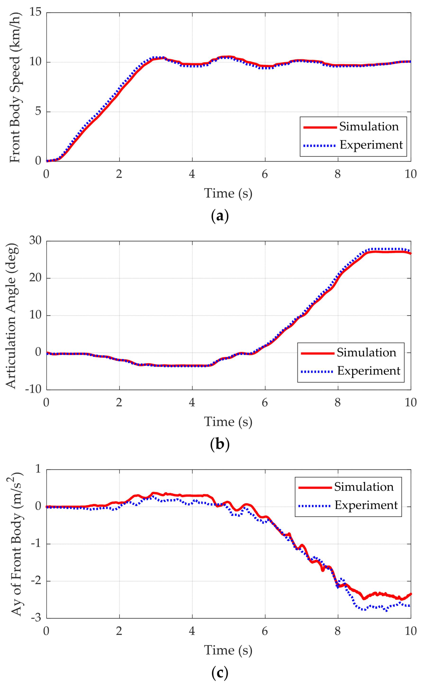
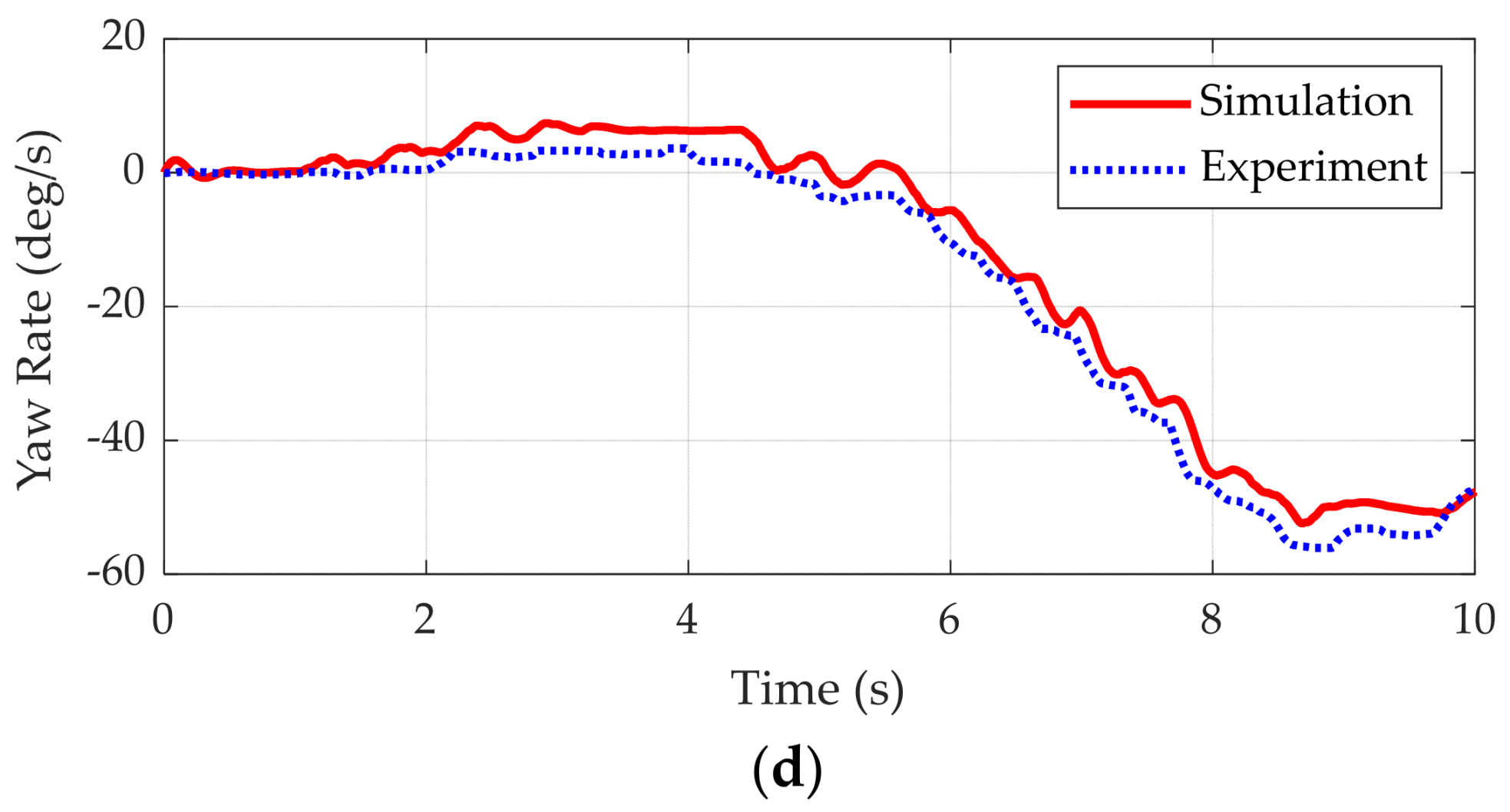
4.1. Model Validation with Experimental Data

The parameters for the vehicle model are given in Table 1. These data were measured from the real AERS, as given in Figure 1. As shown in Table 1, h_r is larger than h_f although the track widths of the front and rear bodies are identical to each other. The experiments were conducted on a high friction road or dry asphalt on a proving ground. As such, the tire–road friction coefficient μ was set to 0.85, which indicates dry asphalt. In the experiment, the lateral acceleration, the speed, and the yaw rate of the front body were measured with the differential GPS, RT1003 from Oxford Technical Solutions [35]. The articulation angle was measured from the steering-angle sensor, Bosch’s Maxus V80, located at the center joint [36]. These signals were fed into the vehicle model implemented on MATLAB/Simulink.

Table 1. Vehicle parameters and values for the AERS.

Parameter	Value	Parameter	Value
mf	778.0 kg	mr	1076.0 kg
Izf	362.0 kg m2	Izr	543.0 kg m2
l2	0.605 m	l3	0.895 m
rwf, rwr	0.28 m	Iwf, Iwr	1.02 kg m2
Kθ	500 Nm/rad	Cθ	200 Nm⋅s/rad
tf	0.93 m	tr	0.93 m
hf	1.2 m	hr	1.4 m
Cx	65,673 N/rad	Cy	60,892 N/rad
μ	0.85

Figure 8 shows the simulation results of the vehicle model and experimental data. In Figure 8a,b, the red solid lines represent the reference articulation angle and the reference speed measured from experiment, respectively. As shown in Figure 8a,b, the vehicle model with the speed and steering controllers can follow the reference speed and articulation angle. As shown in Figure 8c,d, the simulation results of the vehicle model, i.e., the lateral acceleration and the yaw rate of the front body, are well fitted with the experimental data. From these results, it can be shown that the vehicle model implemented in MATLAB/Simulink is valid for use in the simulation.

Figure 8. Simulation results and comparison with experimental data. (a) Speed command of front body and simulation result of the speed controller; (b) Articulation angle command and simulation result of the steering controller; (c) Lateral accelerations of front body from simulation and experiment; (d) Yaw rates of front body from simulation and experiment.

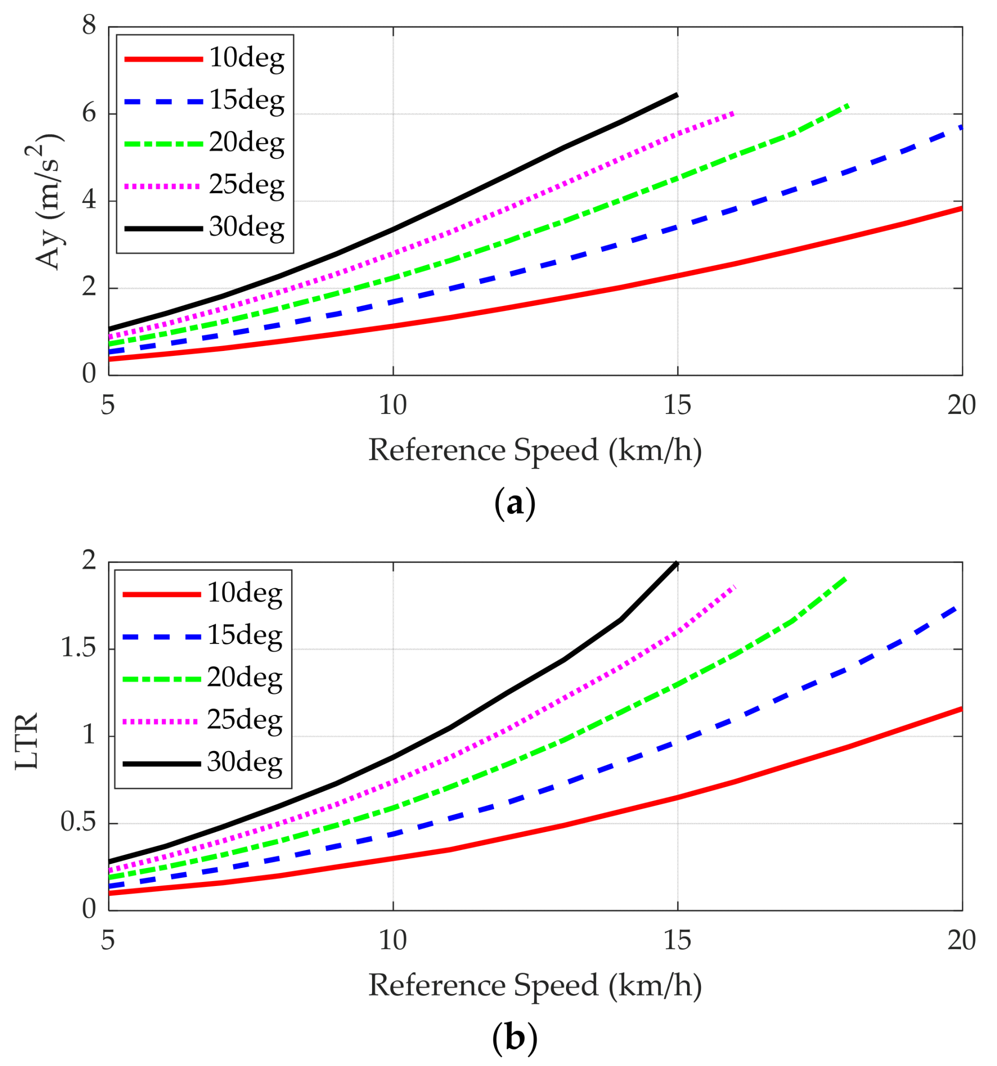
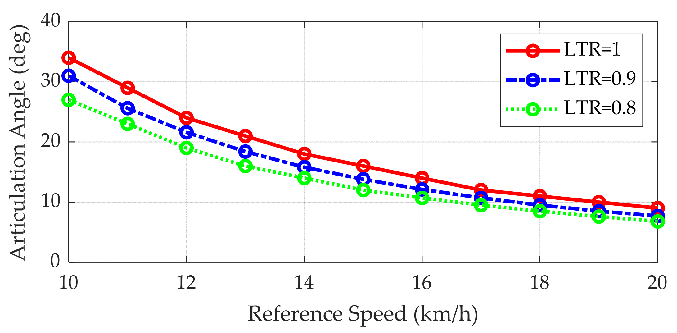
4.2. Analysis on Rollover Propensity with Open-Loop Steering

In this subsection, the rollover propensity of the AERS is analyzed with open-loop steering under a constant speed. The reference speed, v_ref, is set from 5 to 20 km/h with the interval of 1 km/h. The tire–road friction coefficient is set to 0.85, which indicates dry asphalt. The steering angle, i.e., the reference articulation angle, θ_ref, is set from 5 to 30°, with an interval of 5°. These values are kept constant for the simulation period. As such, this is a J-turn maneuver under constant speed. As an output, the maximum of the lateral acceleration and LTR between the front and rear bodies are obtained.

Figure 9 shows the simulation results of open-loop steering under constant speed. In Figure 9b, it can be regarded that the AERS rolls over if the LTR is larger than 1. For example, if the reference speed is set to 15 km/h and the reference articulation angle is set to 15°, then the AERS will roll over because the LTR is 1. The corresponding lateral acceleration can be found in Figure 9a. For the example, the lateral acceleration is about 3.5 m/s². These results are summarized in Table 2 and Figure 8.

Figure 9. Simulation results of the open-loop steering under constant speed. (a) Maximum of lateral accelerations of the front and rear bodies for each articulation angle. (b) Maximum of LTRs of the front and rear bodies for each articulation angle.

Table 2. The combination of reference speed and articulation angle making LTR_f or LTR_r 1.

vref (km/h)	θref (deg)	ayf (m/s2)	ayr (m/s2)	LTRf	LTRr
18.5	10.0	3.34	3.25	0.88	1.00
15.1	15.0	3.51	3.24	0.91	0.99
13.2	20.0	3.63	3.30	0.96	1.01
11.8	25.0	3.72	3.29	0.98	1.01
10.7	30.0	3.78	3.25	0.99	1.00

Table 2 shows the combination of the reference speed and articulation angle causing the LTRf or LTRr be 1. As shown in Table 2, the lateral acceleration of the rear body is smaller than that of the front one. This is due to the fact that the height of the CoG of the rear body is larger than that of the front one. Moreover, the lateral acceleration of the front body increases, and the LTR of the front body approaches 1 as the reference articulation angle does. On the contrary, the lateral acceleration of the rear body is nearly constant, about 3.25 m/s², when the LTR becomes 1.

Figure 10 shows the rollover threshold with respect to the reference speed and the articulation angle. If the combination of the reference speed and articulation angle is above the solid line in Figure 10, then the LTR is larger than 1, which means that the AERS rolls over. Because the AERS is an autonomous vehicle, the reference articulation angle is determined by a driver model, i.e., the pure pursuit method in this paper. As such, the only control variable that is available for rollover prevention is the reference speed. For this reason, the reference speeds derived from Equation (28) and Figure 10 are used as a threshold in the rollover prevention schemes using Method#1 and Method#2, respectively.

Figure 10. Rollover threshold obtained from simulation with respect to the reference speed and articulation angle.

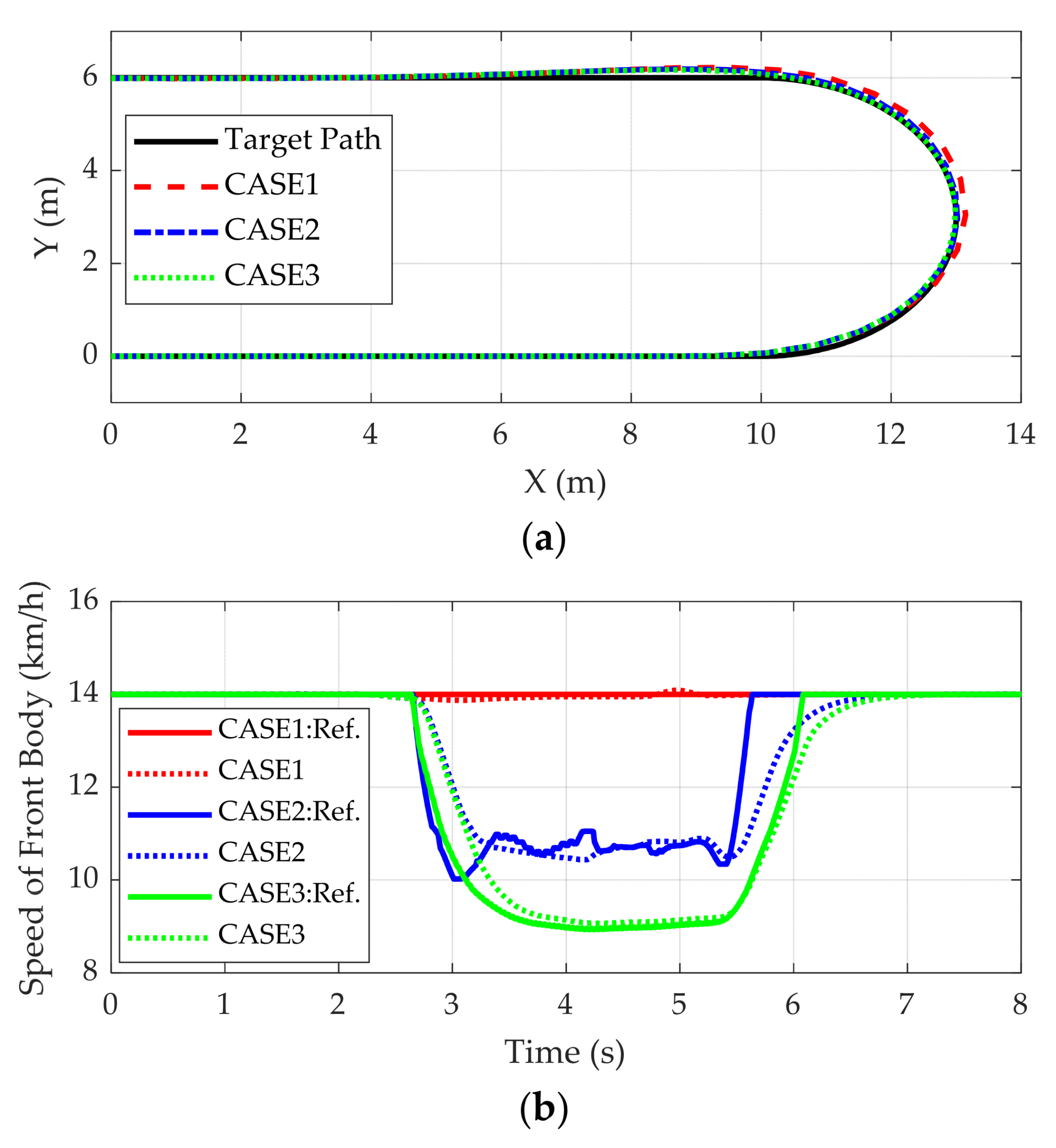
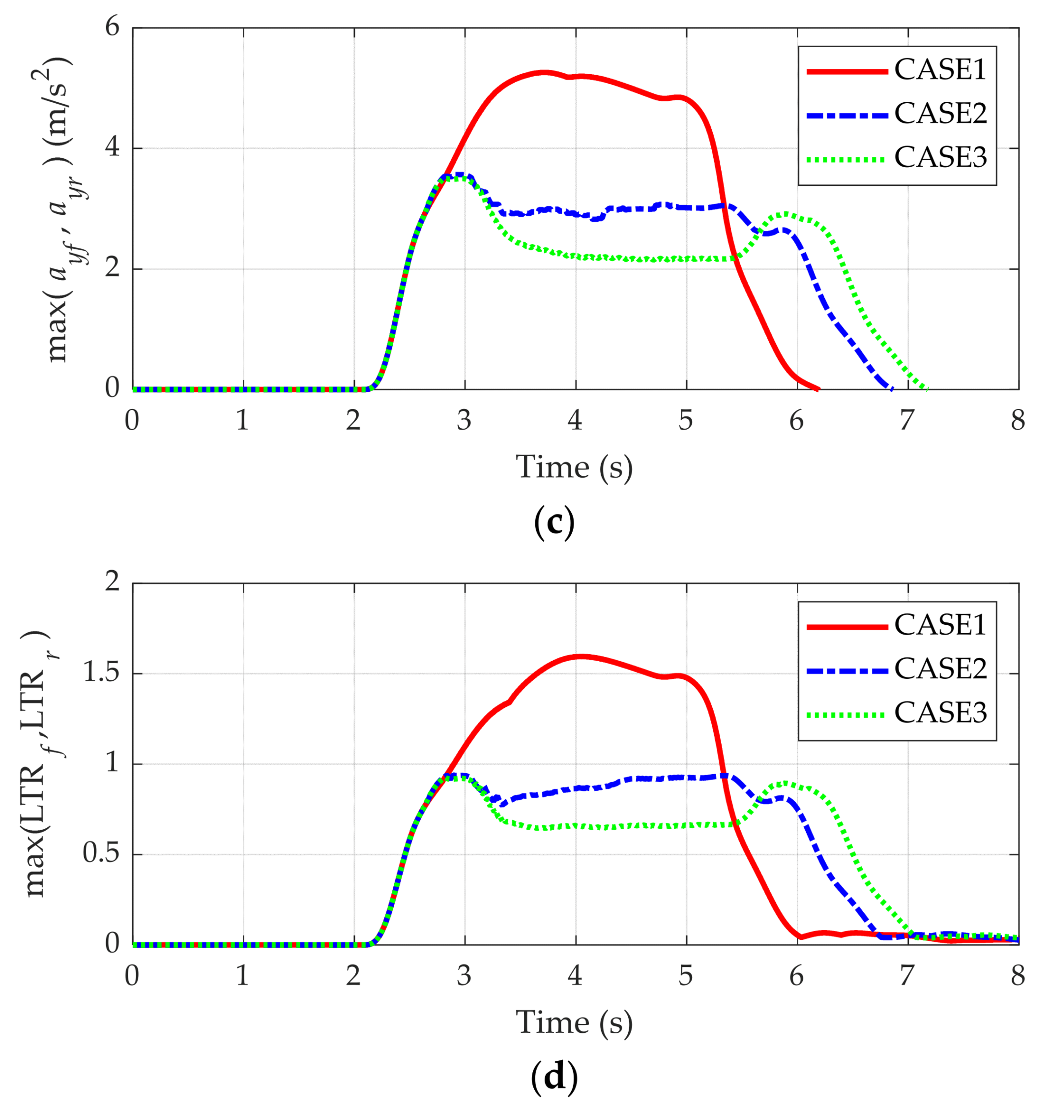
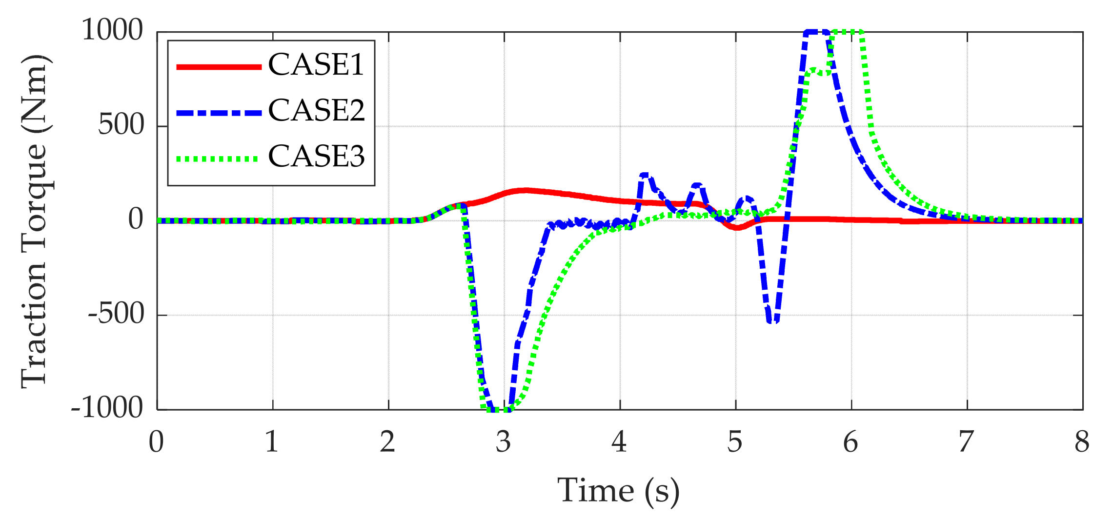
4.3. Rollover Prevention Control with Closed-Loop Steering

To check the effectiveness of the proposed rollover prevention scheme, a simulation was done using closed-loop steering on a U-shaped path. The radius of the path was set to 3 m, and the reference speed was set to 14 km/h. To generate the articulation angle needed to follow the path, the pure pursuit method was adopted. The threshold of the lateral acceleration used to activate the rollover prevention scheme was set to 3.0 m/s². The articulation angle threshold was set to 10°. The tire–road friction coefficient was set to 0.85, which indicates dry asphalt. For comparison, three cases are considered. CASE1 represents the AERS without any rollover prevention schemes. CASE2 and CASE3 are the AERSs with the rollover prevention schemes using Method#1 and Method#2 for reference speed generation, respectively. When using Method#2, the reference speed is calculated from the dotted line of LTR = 0.8 in Figure 8.

Figure 11 and Figure 12 show the simulation results and control inputs for each case, respectively. As shown in Figure 11a, the AERS follows the given path well, regardless of the use of the rollover prevention scheme. The maximum offset from the reference path is 0.361 m. As shown in Figure 11b,c, the rollover prevention scheme was activated when the lateral acceleration became larger than 3.0 m/s². Through the rollover prevention schemes, the reference speed decreased to 11 km/h for CASE2 and to 9 km/h for CASE3. As shown in Figure 11b, the speed controller can follow the reduced reference speed. As a result, the lateral acceleration and LTR were reduced to 3.0 m/s² and 0.9, respectively. After cornering, the rollover prevention scheme was deactivated, and the reference speed increased to the original value. As shown in Figure 8, CASE3 shows the best performance for rollover prevention because it generated the lowest reference speed.

Figure 11. Simulation results of the rollover prevention scheme. (a) Trajectories for each case; (b) Reference and real speeds for each case; (c) Maximum of lateral accelerations of the front and rear bodies for each case; (d) Maximum of LTRs of the front and rear bodies for each case.

Figure 12. Traction/braking torques for each case.

In Figure 11b, the convergence speed of the vehicle speed to the reference one can be accelerated by increasing the gain K_v in (24). In this simulation, K_v was set to 5. However, the larger the gain K_v, the larger the chattering in the traction/braking torques. As such, it is not recommended that K_v is set to a larger value of about 10. For CASE2, there is small chattering in the traction torque, as shown in Figure 12. This is caused by the fact that the lateral acceleration was fed into the reference speed, as given in Equation (28). On the contrary, for CASE3, there is smaller chattering in the traction/braking torque because the lateral acceleration or LTR was not fed into the reference speed. As such, CASE3 is preferable to CASE2 in view of durability.

5. Conclusions

This paper presented the rollover prevention scheme for the AERS. Since the AERS has a single motor in its rear wheels, it is not necessary to separate the dynamics of the left and right wheels. For the reason, the AERS was modeled with a bicycle model with the Dugoff tire model. With the vehicle model, the path tracking and speed controllers were designed for the purposes of following a pre-defined path and speed profile, respectively. As a rollover index, LTR was adopted. For rollover prevention, two reference speed generators were proposed. With the vehicle model, a simulation was conducted in order to analyze the rollover propensity of the AERS. With the analysis results, the simulation was done to check the effectiveness of the proposed rollover prevention schemes. From the simulation results, it can be concluded that the proposed rollover prevention scheme can effectively prevent the AERS from rolling over. The proposed scheme in in the process of being tested on a real AERS. After the tests are completed, the experiment results will be able to be reported.

References

- Peel, G.; Michielen, M.; Parker, G. Some aspects of road sweeping vehicle automation. In Proceedings of the 2001 IEEE/ASME International Conference on Advanced Intelligent Mechanics, Como, Italy, 8–12 July 2001; pp. 337–342. [Google Scholar]
- SAE. Surface Vehicle Standard, Self-Propelled Sweepers and Cleaning Equipment (J2130); SAE Inc.: Warrendale, PA, USA, 1977. [Google Scholar]
- Xu, H.; Xiao, J.; Feng, Y. Development and research status of road cleaning vehicle, International Conference on Electrical Automation and Mechanical Engineering. J. Phys. Conf. Ser. 2020, 1626, 012153. [Google Scholar] [CrossRef]
- Windecker, A.; Ruder, A. Fule economy, cost and greenhouse gas results for alternative fuel vehicles in 2011. Transp. Res. Part D 2013, 23, 33–40. [Google Scholar] [CrossRef]
- Hannan, M.A.; Hoque, M.M.; Mohamed, A.; Ayob, A. Review of energy storage systems for electric vehicle applications: Issues and challenges. Renew. Sustain. Energy Rev. 2017, 69, 771–789. [Google Scholar] [CrossRef]
- Donati, L.; Fontanini, T.; Tagliaferri, F.; Prati, A. An energy saving road sweeper using deep vision for garbage detection. Appl. Sci. 2020, 10, 8146. [Google Scholar] [CrossRef]
- Budich, R.; Hübner, M. Vehicle simulation of an electric street sweeper for substitution analysis. In Internationales Stuttgarter Symposium, Automobil- und Motorentechnik; Spinger: Berlin/Heidelberg, Germany, 2016; pp. 673–690. [Google Scholar]
- Zeng, D.; Yu, Z.; Xiong, L.; Fu, Z.; Li, Z.; Zhang, P.; Leng, B.; Shan, F. HFO-LADRC lateral motion controller for autonomous road sweeper. Sensors 2020, 20, 2274. [Google Scholar] [CrossRef] [PubMed]
- Dou, F.; Liu, W.; Huang, Y.; Liu, L.; Meng, Y. Modeling and path tracking for articulated steering vehicles. In Proceedings of the 2017 Chinese Automation Congress (CAC), Jinan, China, 20–22 October 2017; pp. 5263–5268. [Google Scholar]
- Xiong, L.; Fu, Z.; Zeong, D.; Leng, B. An optimized trajectory planner and motion controller framework for autonomous driving in unstructured environments. Sensors 2021, 21, 4409. [Google Scholar] [CrossRef]
- Excell, J. UK Engineers to Develop Autonomous Electric Street Sweeper. Available online: https://www.theengineer.co.uk/autonomous-electric-street-sweeper/ (accessed on 14 October 2021).
- Autonomous Sweeper from Berlin Startup Approved for Public Road Use in Singapore. Available online: https://www.prnewswire.com/news-releases/autonomous-sweeper-from-berlin-startup-approved-for-public-road-use-in-singapore-301208765.html (accessed on 15 January 2021).
- Self-Driving Road Sweepers to Go on Trial at One-North, NTU and CleanTech Park in Jurong. Available online: https://www.channelnewsasia.com/singapore/self-driving-road-sweepers-trial-ntu-one-north-cleantech-park-407061 (accessed on 14 January 2021).
- Boschung, Urban-Sweeper S2.0 Autonomous. Available online: https://www.boschung.com/product/urban-sweeper-s2-0-autonomous/ (accessed on 14 October 2021).
- Korea IT News, Gwangju-Si and Korea Institute of Industrial Technology to Introduce Two Unmanned Special Vehicles Next Month. Available online: https://english.etnews.com/20201118200004 (accessed on 20 November 2020).
- Lei, T.; Wang, J.; Yao, Z. Modelling and stability analysis of articulated vehicles. Appl. Sci. 2021, 11, 3663. [Google Scholar] [CrossRef]
- Yin, Y.; Rakheja, S.; Yang, J.; Boileau, P.-E. Design optimization of an articulated frame steering system. Proc. Inst. Mech. Eng. Part D J. Automob. Eng. 2017, 232, 1339–1352. [Google Scholar] [CrossRef]
- Azad, N.L.; Khajepour, A.; Mcphee, J. Robust state feedback stabilization of articulated steer vehicles. Veh. Syst. Dyn. 2007, 45, 249–275. [Google Scholar] [CrossRef]
- Xu, T.; Ji, X.; Shen, Y. A novel assist-steering method with direct yaw moment control for distributed drive articulated heavy vehicle. Proc. Inst. Mech. Eng. Part K J. Multi-Body Dyn. 2020, 234, 214–224. [Google Scholar]
- Paden, B.; Cap, M.; Yong, S.Z.; Yershov, D.; Frazzoli, E. A survey of motion planning and control techniques for self-driving urban vehicles. IEEE Trans. Intell. Veh. 2016, 1, 33–55. [Google Scholar] [CrossRef] [Green Version]
- Yurtsever, E.; Lambert, J.; Carballo, A.; Takeda, K. A survey of autonomous driving: Common practices and emerging technologies. IEEE Access 2020, 8, 58443–58469. [Google Scholar] [CrossRef]
- Shiroma, N.; Ishikawa, S. Nonlinear straight path tracking control for an articulated steering type vehicle. In Proceedings of the ICROS-SICE International Joint Conference 2009, Fukuoka, Japan, 18–21 August 2009; pp. 2206–2211. [Google Scholar]
- Yao, W.; Pang, Z.; Chi, R.; Shao, W.; Yang, D. Intelligent sweeper path tracking control based on optimal iterative learning. In Proceedings of the 2020 IEEE 9th Data Driven Control and Learning Systems Conference (DDCLS), Liuzhou, China, 20–22 November 2020; pp. 600–605. [Google Scholar]
- Yim, S. Design of a preview controller for vehicle rollover prevention. IEEE Trans. Veh. Technol. 2011, 60, 4217–4226. [Google Scholar] [CrossRef]
- Yim, S.; Park, Y.; Yi, K. Design of active suspension and electric stability program for rollover prevention. Int. J. Automot. Technol. 2010, 11, 147–153. [Google Scholar] [CrossRef]
- Yoon, J.; Yim, S.; Cho, W.; Koo, B.; Yi, K. Design of an unified chassis controller for rollover prevention, manoeuvrability and lateral stability. Veh. Syst. Dyn. 2010, 48, 1247–1268. [Google Scholar] [CrossRef]
- Qian, X.; Wang, C.; Zhao, W. Rollover prevention and path following control of integrated steering and braking systems. Proc. Inst. Mech. Eng. Part D J. Automob. Eng. 2020, 234, 1644–1659. [Google Scholar] [CrossRef]
- Tian, Y.; Huang, K.; Cao, X.; Liu, Y.; Ji, X. A hierarchical adaptive control framework of path tracking and roll stability for intelligent heavy vehicle with MPC. Proc. Inst. Mech. Eng. Part D J. Automob. Eng. 2020, 234, 2933–2946. [Google Scholar] [CrossRef]
- Xu, T.; Wang, X. Roll stability and path tracking control strategy considering driver in the loop. IEEE Access 2021, 9, 46210–46222. [Google Scholar] [CrossRef]
- Shao, K.; Zheng, J.; Huang, K. Robust active steering control for vehicle rollover prevention. Int. J. Model. Identif. Control. 2019, 32, 70–84. [Google Scholar] [CrossRef]
- Gao, L.; Jin, C.; Liu, Y.; Ma, F.; Feng, Z. Hybrid model-based analysis of underground articulated vehicles steering characteristics. Appl. Sci. 2019, 9, 5274. [Google Scholar] [CrossRef] [Green Version]
- Ataei, M.; Khajepour, A.; Jeon, S. A general rollover index for tripped and un-tripped rollovers on flat and sloped roads. Proc. Inst. Mech. Eng. Part D J. Automob. Eng. 2017, 233, 304–316. [Google Scholar] [CrossRef]
- Cho, W.; Yoon, J.; Kim, J.; Hur, J.; Yi, K. An investigation into unified chassis control scheme for optimised vehicle stability and maneuverability. Veh. Syst. Dyn. 2008, 46, 87–105. [Google Scholar] [CrossRef]
- Omead, A. Integrated Mobile Robot Control. In Technical Report CMU-RI-TR-90-17; Carnegie Mellon University Robotics Institute: Pittsburgh, PA, USA, May 1990. [Google Scholar]
- Oxford Technical Solutions Ltd. RT1003, The Compact INS for Space Constrained Vehicle Testing. 2021. Available online: https://www.oxts.com/products/rt1003-lightweight-gnss-ins-for-automotive-testing/ (accessed on 5 November 2021).
- Robert Bosch GmbH. Steering-angle Sensor. 2021. Available online: https://www.bosch-mobility-solutions.com/en/solutions/sensors/steering-angle-sensor/ (accessed on 5 November 2021).
Publisher’s Note: MDPI stays neutral with regard to jurisdictional claims in published maps and institutional affiliations. |
© 2021 by the authors. Licensee MDPI, Basel, Switzerland. This article is an open access article distributed under the terms and conditions of the Creative Commons Attribution (CC BY) license (https://creativecommons.org/licenses/by/4.0/).