Custom Face Classification Model for Classroom Using Haar-Like and LBP Features with Their Performance Comparisons

Abstract

Face detection by electronic systems has been leveraged by private and government establishments to enhance the effectiveness of a wide range of applications in our day to day activities, security, and businesses. Most face detection algorithms that can reduce the problems posed by constrained and unconstrained environmental conditions such as unbalanced illumination, weather condition, distance from the camera, and background variations, are highly computationally intensive. Therefore, they are primarily unemployable in real-time applications. This paper developed face detectors by utilizing selected Haar-like and local binary pattern features, based on their number of uses at each stage of training using MATLAB’s trainCascadeObjectDetector function. We used 2577 positive face samples and 37,206 negative samples to train Haar-like and LBP face detectors for a range of False Alarm Rate (FAR) values (i.e., 0.01, 0.05, and 0.1). However, the study shows that the Haar cascade face detector at a low stage (i.e., at six stages) for 0.1 FAR value is the most efficient when tested on a set of classroom images dataset with 100% True Positive Rate (TPR) face detection accuracy. Though, deep learning ResNet101 and ResNet50 outperformed the average performance of Haar cascade by 9.09% and 0.76% based on TPR, respectively. The simplicity and relatively low computational time used by our approach (i.e., 1.09 s) gives it an edge over deep learning (139.5 s), in online classroom applications. The TPR of the proposed algorithm is 92.71% when tested on images in the synthetic Labeled Faces in the Wild (LFW) dataset and 98.55% for images in MUCT face dataset “a”, resulting in a little improvement in average TPR over the conventional face identification system.

1. Introduction

Face detection using electronic technology aims to determine the presence of the face(s) in a given digital image or video. The process may proceed to identify the face(s) detected depending on the area of application. Face detection by electronic systems has been leveraged by private and government establishments to enhance the effectiveness of a wide range of applications in our day to day activities, security, and businesses. This technology’s attractiveness lies in its non-invasive and discreet nature [1], ease of application, rapid predictiveness, sensitivity to confounding features, and potentially low cost. All of these are made possible due to the developments in computer software and hardware capabilities such as the GPUs (Graphical Processing Unit) [2], multicamera systems [3], and the emerging face detection algorithms.

The emerging algorithms, which represent the software aspect of the technology, have been divided into different categories, such as feature-based, learning-based, and hybrid (i.e., feature and learning-based). However, this classification depends on how the method detects faces. In our opinion, little or no reference was given to their best areas of application. Furthermore, the constrained and unconstrained conditions, leading to the limitation of this algorithm’s performance, are not viewed as an advantage towards their areas of application [4].

Most face detection algorithms that can reduce the problems posed by unconstrained environmental conditions such as unbalanced illumination, weather condition, distance from the camera, and background variation are highly computationally intensive [5]. Therefore, they are largely unemployable in real-time applications, especially for low power electronic and sensor devices.

Educational application of face detection technology mostly requires simultaneous face detection applications such as classroom student attendance system, students and staff identity verification, laboratories, and classroom accessibility control. Testing the detection capability of some of the face detection algorithms gives room for determining the best applicable algorithm in educational settings.

Several approaches to face detection algorithms have been described in the literature. The face detection work of Viola and Jones [6] used Haar-like features selection using a cascade classifier. Leinhart and Maydt [7] modified the Haar-like feature used by Viola and Jones for improvement. Li et al. [8] proposed a learning method of detecting faces in an image using the Viola–Jones algorithm. Ojala et al. [9] used local binary pattern (LBP) features extracted from the local neighborhood in place of Haar-like features employed by Viola and Jones, and similarly, Ahonen et al. [10] also used LBP for face detection. Levi and Weiss [7] used edge orientation histograms (EOH) to source feature information from an image. Furthermore, efforts have been made by some researchers to compare some of these approaches. Kortli et al. [11] compared the performance of three face descriptors (i.e., LBP, LBPHistogram (LBPH), and Histograms of Oriented Gradients (HOG)) using the FERET dataset. Kadir et al. [12] compared the performance of Haar-like cascade and LBP using still image samples from three face databases (i.e., Colour FERET [13], Taarlab [14], and MIT CBCL [15] databases). Guennouni et al. [16] used Haar-like cascade and LBP approaches to detect faces, hand gestures, and pedestrians. This work was done to determine the comparative performance of the two approaches for embedded devices. The Haar-like cascade achieved greater accuracy (i.e., 96.24%) as compared to LBP (i.e., 94.75%). Adouani et al. [17] performed a comparative study on three face detection approaches (Haar-like cascade, LBP, and HOG with Support Vector Machine). The application was tested on the general database face video sequence.

Most of these approaches carried out comparative studies on the general face detection databases without indicating a specific application area’s performance index. In addition to that, the effect of the false alarm rate and the number of training stages on the algorithms’ performance has not been reported explicitly.

Successful implementation of most face detection algorithms is performed with OpenCV and Dlib using Python or C programming, or MATLAB using the computer vision toolbox. For example, Alionte and Lazar [18] created a Haar-like cascade face detector based on the Viola–Jones algorithm using MATLAB’s computer vision toolbox. Adouani et al. [17] implemented a face detection using Haar-like cascade, LBP, and HOG with SVM in OpenCV and Dlib using Python programming. However, a custom cascade classifier can be implemented in MATLAB for any of the commonly used approaches for better object detection [19].

This paper presents a practical custom cascade face classifier for two approaches (i.e., Haar-like and LBP) using the trainCascadeObjectDetector function in MATLAB. The resulting cascade classifier for approaches, in Extensible Markup Language (XML) format, was tested on classroom databases. Their performances were compared based on True Positive Rate (TPR), False Negative Rate (FNR), False Alarm Rate (FAR), and the number of training stages (NTS) [20]. The paper is structured as follows. Section 2 provides an overview of the main concepts of the trainCascadeObjectDetector function and the definitions of the parameters. Section 3 describes our proposed approach and the procedure involved in using MATLAB’s traincascadeObjectDetector to train a cascade object detector. Section 4 describes the application of the trained CascadeObjectDetector on an image obtained from a classroom image database. Section 5 presents the results and performance analysis of the two trained CascadeObjectDetectors (i.e., for Haar and local binary patterns (LBP)), and the discussions are presented in Section 6. Finally, the summary, conclusions, and the future direction of the research work are discussed in Section 7.

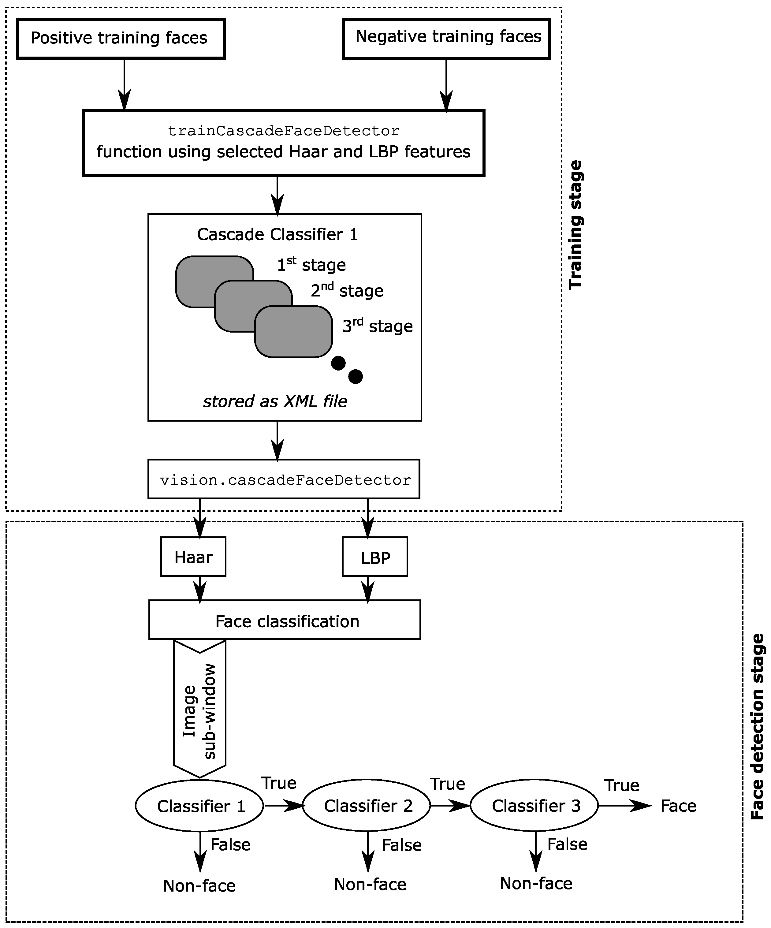
2. Cascade Object Detector

The trainCascadeObjectDetector is a classifier function for vision. CascadeObjectDetectors system object is present in MATLAB’s computer vision toolbox. It is used to create a custom classifier for detecting categories of objects whose aspect ratio does not change (fixed), such as faces, human full-body, cars, body features, plate numbers. Cascade object detector is a group of cascade classifiers arranged in stages. Each stage consists of decision stumps (weak learners). Each stage selects smaller numbers of features using a technique called boosting (i.e., Adaboost). Adaboost creates an accurate complex classifier by combining the average weight of the decision taken by the weak classifiers.

AdaBoost Algorithm for Selecting Features

For example, let us consider the Adaboost classifier’s learning as a suggestion of a group of experts. The classification result by each expert $E_n$ for the input $x_i$ is expressed as $E_n\left(x_i\right)$. To differentiate between the training vector of two outcomes, $E_n\left(x_i\right)$ can only accept two results that are represented as +1 or −1, i.e., $E_n\left(x_i\right)\in \{-1,+1\}$. The collective opinion of the experts is denoted as $K\left(x_i\right)$. It represents the linear combination of the weighted sum of expert suggestions, which can be expressed as follows:

$$K\left(x_i\right)=w_1{E}_1\left(x_i\right)+w_2{E}_2\left(x_i\right)+\cdots +w_n{E}_n\left(x_i\right)$$

(1)

where $E_1\left(x_i\right),E_2\left(x_i\right),\dots ,E_n\left(x_i\right)$ represent the decisions from n experts and $w_1,w_2,\dots ,w_n$ are the weights given to each expert suggestion [21]. The procedural steps of the Adaboost algorithm for classifier learning of features are given as follows:

• Given a training data with n pairs of images $(x_i,y_i)$, where $x_i$ is a positive or negative image, and $y_i$ is the label allotted to each image. The value for positive images is 1, and that of negative images is 0.
• Initializing weights $w_{1,i}=\frac{1}{2m},\frac{1}{2l}$ for positive and negative images, where m and l are the number of negative and positive images, respectively.
• For $t=1,\dots ,T$, where T is the number of stages of training and n pairs of images:
  • The weights are normalized as $w_{i,t}\leftarrow w_{i,t}/{\sum }_{j=1}^n{w}_{i,j}$
  • Applying a single feature, for every feature, j, train a classifier $h_j$, the weighted error is evaluated as $e_i={\sum }_i{w}_i|h_i\left(x_i\right)-y_i|$
  • Select the classifier $h_t$ that has the lowest error $e_t$.
• Update the weight $w_{t+1,i}=w_{t,i}{\beta }_t^{1-e_i}$, where $e_i=0$ when $x_i$ is classified correctly, $e_i=1$ otherwise and ${\beta }_t=e_t/(1-e_t)$.
• The final strong classifier, which is the combination of the weak classifiers, is expressed as follows:

  $$h\left(x\right)=\left\{\begin{array}{cc}1\hfill & \sum _{t=1}^T{\alpha }_t{h}_t\left(x\right)\ge \frac{1}{2}\sum _{t=1}^T{\alpha }_t\hfill \\ 0\hfill & \mathrm{otherwise}\hfill \end{array}\right.$$

  where ${\alpha }_t={log}_{10}(1/{\beta }_t)$.

The outcome of each stage of a weak classifier can be either a positive or negative value. The positive value means a face is located on the image, whereas the negative value indicates that no face is found. In the case of a negative outcome, the detector moves the sliding window to the next location. If the outcome is positive, the classifier moves the region to the next stage and indicates that a face is in the current window region. A larger percentage of the image contains no object of interest on presupposition, the stages programmed to do away with negative outcomes faster. On this note, some common terms need to be defined:

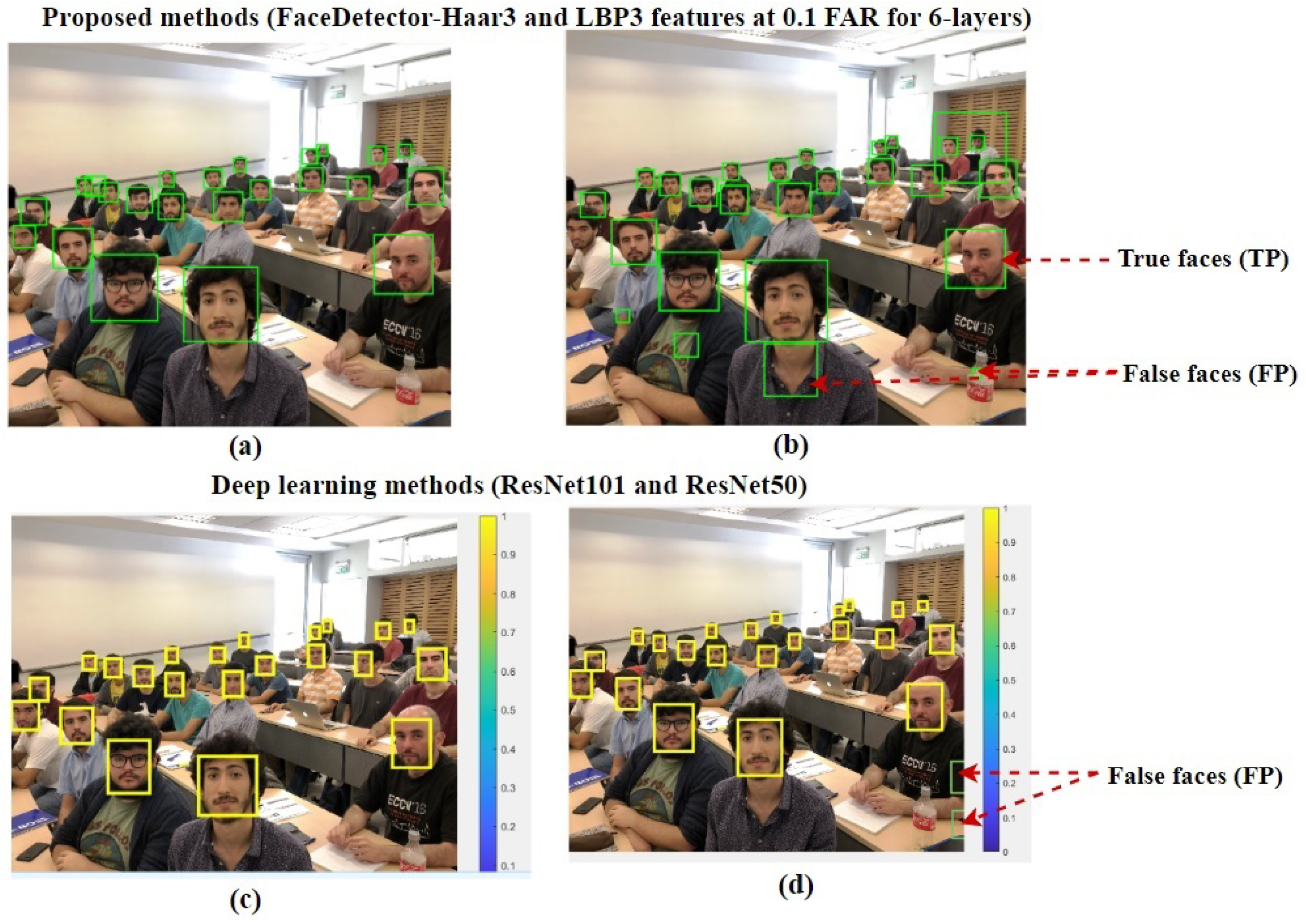
• True-positives (TP): They are an actual object of interest that are correctly classified. The rate of the correctly classified object/faces can be determined as [20]:

  $$\mathrm{True-positives} \mathrm{rate} \left(\mathrm{TPR}\right)=\frac{\mathrm{TP}}{(\mathrm{TP}+\mathrm{FP})}$$

  (2)
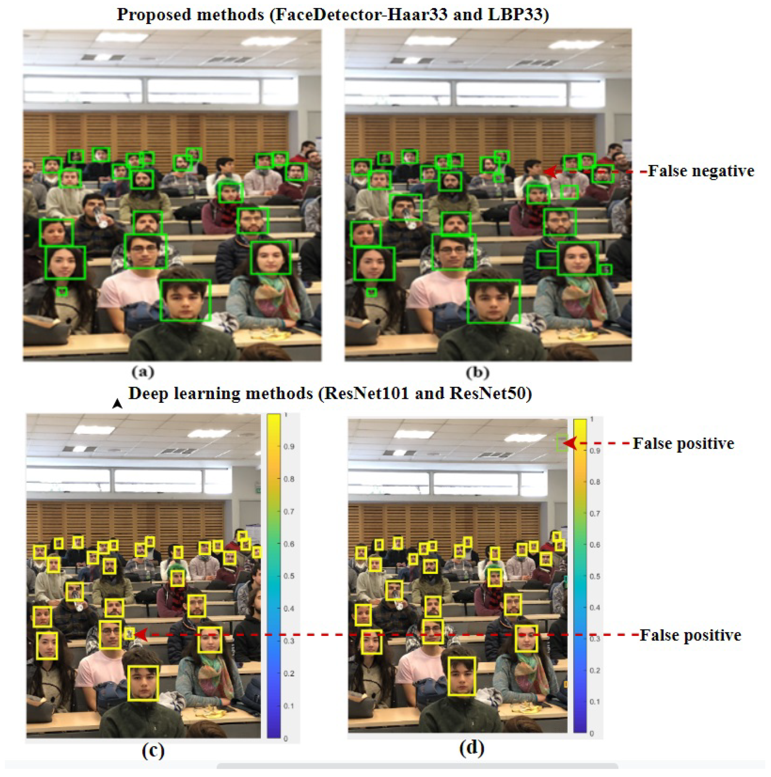
• False-positives (FP): They are the non-object of interest that are wrongly classified as the true object.
• False-negatives (FN): They are an actual object of interest wrongly classified as negative. The False Negative Rate (FNR) can be obtained using Equation (3):

  $$\mathrm{False-negatives} \mathrm{rate} \left(\mathrm{FNR}\right)=\frac{\mathrm{FN}}{(\mathrm{FN}+\mathrm{TP})}$$

  (3)

3. Our Proposed Method

Most custom trained cascade object detectors failed to identify the effect of the FAR, Number of Training Stages (NTS), and the frequency and performance of the feature usage at each stage of the cascade on the overall performance of the cascade object detector.

Figure 1 describes the flow of the proposed approach. In this design, Haar features are selected based on their usage at each stage [22], and the training parameters were varied to obtain the best settings. To obtain a better trained cascade object detector result, the false-negative rate should be low in value (i.e., in between 0 to 1) so that more faces can be detected at the initial stages. Subsequent stages correct the mistakes of the previous ones, which give room for proper examination before marking an object as negative.

Alexandre et al. [22] demonstrated that the central features and the vertical-double features had less than 5% usage at the detection window for each stage of the cascade. While rotated feature and the horizontal-double features are the most commonly used based on their position, area, and width to height ratio for the region of interest in face detection (the nose, eyes, and the cheeks). Based on this fact, features with less usage (vertical double and central) are eliminated for features that focused on detecting the eye, nose, and cheek. In this approach, horizontal double, rotated, and crossed features are employed, as shown in Figure 2.

3.1. Feature Evaluation

The choice between the pixel and feature as a common characteristic of object detection is always a contention. Features have more advantages over pixels. Features can take measures to obtain make-shift domain knowledge that may require a large amount of training data to learn. Additionally, feature-based systems are more computationally efficient than pixel-based [6]. Therefore, Haar and LBP features of the trainCascadeObjectDetector function were employed because of their better representation of fine-scale texture, which suits face detection.

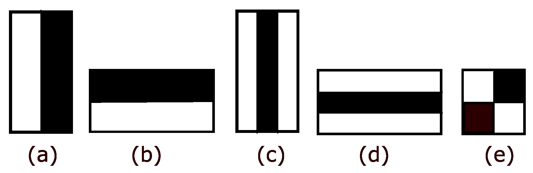
3.1.1. Haar-Like Features

Haar has been a common feature employed by many researchers for object detection [6,23]. Viola–Jones used Haar-like rectangle features adapting the idea (from the work of Papageoriou et al. [23]) of using Haar-like wavelets. Figure 2 shows the examples of the rectangle Haar-like feature placed around the region of the image to detect faces. There are two-rectangle features (vertical and horizontal) as shown in Figure 2a,c, a three-rectangle feature in Figure 2e, and a single four-rectangle feature in Figure 2h. They are used to determine the common attributes of the face because the region of the eyes is believed to be darker than that of cheeks, while that of the nose is brighter. The sum of the pixels that lie within the white rectangle is subtracted from the sum of the pixels in the grey rectangle to determine the difference in the contrast region.

Alexandre et al. [22] showed the percentage usage of each of these features in face detection. The features with the frequent percentage of use are the horizontal-double and horizontal-triple features and their rotated versions (i.e., 45.771%, 8.70%, 7.068%, and 8.043%), vertical-double rotated type (9.660%), vertical-triple feature and its rotated version (7.764% and 10.885%), and the four rectangle features (34.647%), respectively. Consequently, features whose geometric values (position, area, and width-to-height ratio) are not used at the final stages of the cascade are eliminated. Therefore, only those features are employed to optimize the speed of processing and the detection rate.

Furthermore, the Haar-like features can be classified into five types, left-right, top-bottom, horizontal-middle, vertical-middle, and diagonal, as shown in Figure 3. By rotating the left-right and vertical-middle in anti-clockwise produce top-bottom and horizontal-middle, respectively. These features are used to detect the presence of faces by sliding a fixed-size window of the feature at all scales over the input image. Taken a detector of $24\times 24$ base resolution, the Haar-like feature obtainable from it is 162,336, which is quite large in terms of computational time required to resolve. An intermediate representation for the image, which is called an integral image, is used to speed up the feature’s extraction process.

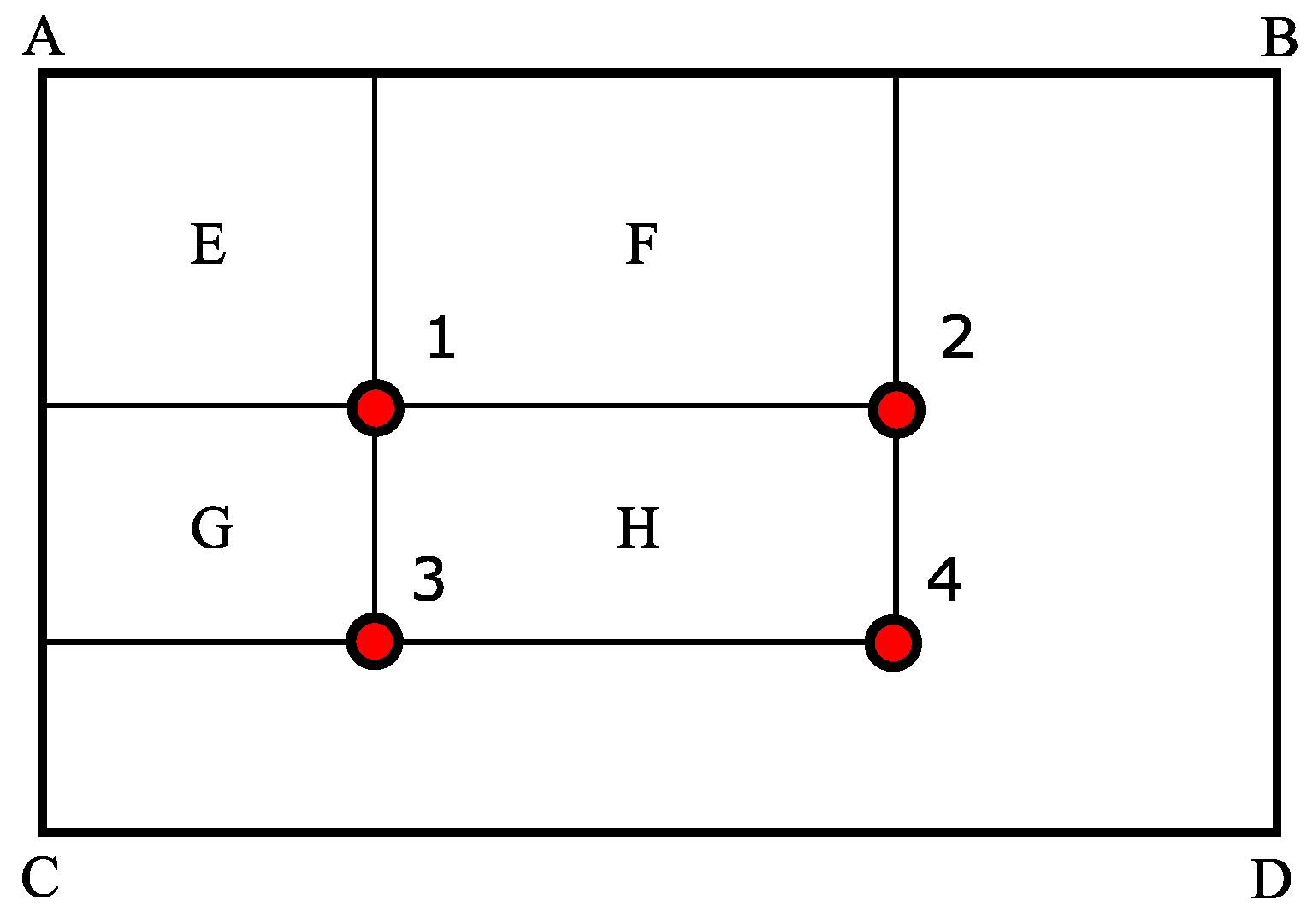
3.1.2. Integral Image

An intermediate rendition of the image is necessary to speed up the features’ location and extraction process. An integral image is a new image rendition that makes feature evaluation very fast. By referring to Figure 4 as an example, to obtain the sum of pixels in a rectangle ABCD, an integral part of it (EFGH) is taken to compute the pixel value. The integral value at location 1 is the sum of the pixel on the rectangle E, at location 2 is the sum of the pixel at E + F, at location 3 is E + F + G and at location 4 is the sum of the pixels at E + F + G + H. The computed sum of the pixel within H is 4 + 1 − (3 + 2).

3.1.3. Attentional Cascade

This approach is described as a chain classifier that is progressively more complex from one stage to another. It has low false-positive rates, thereby rejecting most of the negative windows and then allowing the positive instances shown in Figure 5. It is a cascaded system where the first classifier’s response determines the second classifier’s action, and each stage classifier triggers the next classifier if its output is positive. The classifiers are designed to attain high detection rates. A negative outcome at any stage of the cascade is an automatic rejection of the sub-window. Generally, the learning algorithms (AdaBoost) are used to create the cascade stages by adjusting the threshold value to achieve the minimum number of false negatives possible. However, a lower AdaBoost threshold value produces higher detection rates and higher false-positive rates.

In an attentional cascade, every part of the multiple split windows is a potential input. Each split part of the window is checked at every layer of the cascade whether it is a face, then it will be moved to the next strict classifier or if not, then it will be rejected, and the next window will be supplied to the classifier until all the parts are checked. A successful face is the one that passes through all the layers of the attention cascade.

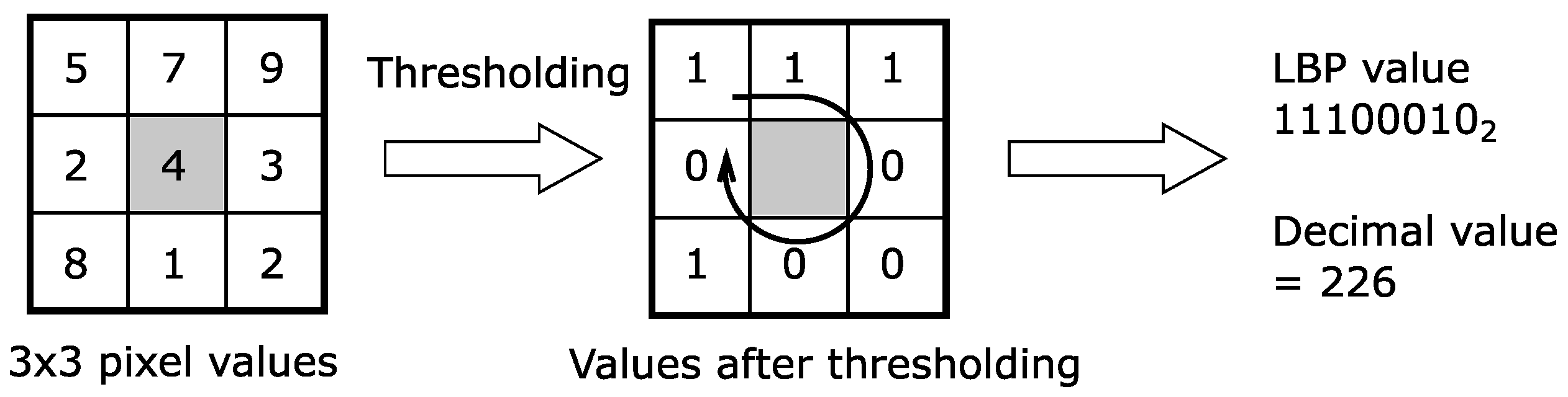
3.1.4. Local Binary Patterns (LBP) Features

This approach is a non-parametric image representation pattern that encodes both local and global facial attributes into a compact feature histogram. LBP was mainly built to analyze texture features [24] but proved very powerful as a tool to describe the structures (local and global) of an image. It has been tried in different application capacities, for instance, motion analysis [25,26], biomedical analysis [27], remote sensing [28], aerial image analysis [29], image and retrieval video [30,31] and many other areas.

The pixels of an image are arranged in LBP format, that is, tagging each pixel with decimal numbers. The format is called Local Binary Patterns or LBP codes. LBP considers the $3\times 3$ neighborhood of each pixel by subtracting the value of the center pixel from its neighbors (8). If the resulting value obtained is a positive number, it is represented as 1, otherwise 0. This procedure will create binary numbers (zeros and ones), which can be combined starting from the top-left in a clockwise direction. The resulting binary numbers are referred to as the local binary patterns. The decimal value obtained after converting the LBP value serves as a label for the pixels. Figure 6 shows a local binary conversion of a $3\times 3$ neighborhood pixel.

4. Cascade Classifier Using the MATLAB’s trainCascadeObjectDetector Function

A simple framework is employed to produce a highly efficient cascade classifier. Cascade classifier training requires a set of positive and negative samples. A region of interest was specified for each positive sample, while that of the negative sample is insignificant. The MATLAB Image labeler was employed in this training to label the positive sample’s region of interest using bounding boxes. This can also be done by setting the resolution of the positive samples to a specific small value (for example, $24\times 24$). A table was produced by the image labeler, which contains the label information of the positive samples. The actions performed by the train cascade detector at each stage are listed as follows:

• Stage One training:

  -

  It calculates the number of positive samples it will use which should less than the number provided

  -

  It generates negative samples from the negative images provided by the user

• Stage Two training:

  -

  Adopt data from stage one

  -

  Classify all positive samples and then get rid of the misclassified negative samples

  -

  Use the same calculated number of positive samples

  -

  Create negative samples from the negative images provided using the sliding window and then adopt false-positive classified samples

• …
• Stage N training:

  -

  Use previous stages

  -

  Classify all positive sample and then get rid of the misclassified negatives

  -

  Use the same calculated numbers of positive samples

  -

  Create negative samples from the negative images provided using the sliding window and then adopt false-positive classified samples

The following function parameters are to be set to optimize the training stages; false-positive rate, the true-positive rate, and the feature type to be employed for the training. By default, the number of negative samples is double that of the positive samples (i.e., the multiplication factor is 2). For this training, the false positive rate, also called as False Alarm Rate (FAR), is varied as 0.01, 0.05, and 0.1. These three values are used to evaluate the effect of FAR on the two approaches’ performance. Although the default value is 0.5, other value in between 0 to 1 (0, 1] can be set. The true positive rate is set to be the default value, which is 0.995; a value between 0 to 1 (0, 1] can be set. MATLAB supports three types of features “Haar-like”, “LBP” and “HOG” for training. For this study, two features were selected (i.e., Haar-like and LBP). We first trained for the Haar-like feature and then the LBP feature. The two custom cascade object detectors were used to test a classroom educational dataset, and their performances are compared.

5. Experimental Results

The set of faces used for the training consists of 2577 labeled faces. The base resolution for the face images is set to be $24\times 24$ pixels, which indicated the minimum size of faces the trained cascade detector can detect. The positive sample faces were obtained from a website during a random search of the world wide web (https://github.com/NVlabs/ffhq-dataset). Figure 7 shows some of the positive sample faces used for the training. The negative samples which represent the non-face sub-windows are 37,206 images.

Each stage of the classifier in the cascade was trained with the 2651 (also of size 24 by 24 pixels) training faces, and 5302 negative samples using the Haar-like and LBP features, respectively. The trained face detectors’ performance is tested using different educational classroom database images obtained from a GitHub website (https://github.com/mackenney/attendance-system-wacv19/tree/master/DB). The analysis was carried out based on the number of faces detected (TP), the True faces that are not detected (FN), the False faces detected (FP), and the time taken to detect the faces (DT). The performance was tested in comparison with that of two pre-trained tiny faces (ResNet 101 and 50) deep learning face detector obtained from Finding Tiny Faces (cmu.edu) [32] using classroom images with a resolution of $3471\times 3024$ and $3798\times 3024$ pixels, respectively.

Table 1. Performance of custom trained Haar-like and LBP features for 0.01, 0.05, and 0.1 false alarm rate (FAR) values and six layers of stages.

Detector	DT	FAR	TP	FN	FP	TPR in %	FNR in %
FaceDetector-Haar1	1.0939 s	0.01	18	4	0	81.82	18.18
FaceDetector-LBP1	0.9724 s	0.01	18	4	0	81.82	18.18
FaceDetector-Haar2	1.1301 s	0.05	20	2	0	90.91	9.09
FaceDetector-LBP2	1.4496 s	0.05	21	1	17	95.45	4.55
FaceDetector-Haar3	1.0555 s	0.10	22	0	1	100.00	0.00
FaceDetector-LBP3	1.2290 s	0.10	21	1	4	95.45	4.55
HR-ResNet101	139.5256 s	-	22	0	1	100.00	0.00
HR-ResNet50	110.1023 s	-	22	0	2	91.67	0.00

Note: FaceDetector-Haar1 and LBP1 is for 0.01, Haar2 and LBP2 is for 0.05, and Haar3 and LBP3 for 0.1 FAR trained cascade for 6-layers.

shows the comparative performance analysis of the two trained detectors (Haar-like and LBP), for six layers of stages, compared to ResNet101 and ResNet50 deep learning (tiny face) model. Figure 8 shows a sample of the faces detected by the corresponding methods.

Table 2. Performance of custom trained Haar-like and LBP features for 0.01, 0.05, and 0.1 false alarm rate (FAR) values and eight layers of stages.

Detector	DT	FAR	TP	FN	FP	TPR in %	FNR in %
FaceDetector-Haar11	1.1454 s	0.01	20	6	1	76.92	23.08
FaceDetector-LBP11	1.0124 s	0.01	21	5	0	80.77	19.23
FaceDetector-Haar22	1.0637 s	0.05	20	6	1	76.92	23.08
FaceDetector-LBP22	1.1136 s	0.05	21	5	0	80.77	19.23
FaceDetector-Haar33	1.0451 s	0.10	21	5	1	80.77	19.23
FaceDetector-LBP33	1.0738 s	0.10	22	4	5	81.48	18.52
HR-ResNet101	56.0617 s	-	24	2	1	95.60	0.08
HR-ResNet50	29.8578 s	-	26	0	1	92.86	0.00

Note: FaceDetector-Haar11 and LBP11 is for 0.01, Haar22 and LBP22 is for 0.05, and Haar33 and LBP33 for 0.1 FAR trained cascade for 8 layers.

shows the performance of the two trained face detectors at eight layers of stages, using Image II. The output samples of the faces detected by the corresponding methods are shown in Figure 9. The performance of the two trained custom cascade face detector classifiers based on the number of cascade layers (6 and 8 stages) for 0.01, 0.05 and 0.1 FAR, and that of the deep learning face cascade classification models are compared using the classroom database images. The performance is as shown in

Table 3. The performance of Haar-like, LBP for 6 and 8 stages compared to deep learning ResNet101 and ResNet50 pretrained models.

	Detector	DT	FAR	TP	FN	FP	TPR	FNR
							in %	in %
Six stages	FaceDetector-Haar1	1.094 s	0.01	18	4	0	81.82	18.18
	FaceDetector-Haar2	1.130 s	0.05	20	2	0	90.91	9.09
	FaceDetector-Haar3	1.056 s	0.10	22	0	1	100.00	0.00
	FaceDetector-LBP1	0.972 s	0.01	18	4	0	81.82	18.18
	FaceDetector-LBP1	1.460 s	0.05	21	1	17	95.45	4.55
	FaceDetector-LBP3	1.229 s	0.10	21	1	4	95.45	4.55
Eight stages	FaceDetector-Haar11	1.145 s	0.01	20	6	1	76.92	23.08
	FaceDetector-Haar22	1.064 s	0.05	20	6	1	76.92	23.08
	FaceDetector-Haar33	1.045 s	0.10	21	5	1	80.77	19.23
	FaceDetector-LBP11	1.012 s	0.01	21	5	0	80.77	19.23
	FaceDetector-LBP22	1.114 s	0.05	21	5	0	80.77	19.23
	FaceDetector-LBP33	1.074 s	0.10	22	4	5	81.48	18.52
Tiny Face	HR-ResNet101 (1)	139.526 s	-	22	0	1	100.00	0.00
(ResNet101 and ResNet50)	HR-ResNet50 (1)	110.102 s	-	22	0	2	91.67	0.00
for	HR-ResNet101 (2)	56.062 s	-	24	2	1	95.60	0.08
Image (1) and (2)	HR-ResNet50 (2)	29.858 s	-	26	0	1	92.86	0.00

.

Our approach was compared with three recently developed approaches (i.e., methods by Chen et al. [33], Kortli et al. [11], and Adouani et al. [17]), based on their achieved true positive rate evaluation (TPR) for the haar and LBP algorithm. The comparison was carried out on the database used by Chen et al. (MUCT face database testing “a” [34] and Labeled Faces in the Wild (LFW) database [35]). Figure 10 shows some samples of the cropped detected faces from MUCT and LFW databases. The results are shown in

Table 4. Comparisons of our approach with three recent approaches using the same database.

Approach	MUCT Dataset		LFW Dataset
	TPR for Haar (%)	TPR for LBP (%)	TPR for Haar (%)	TPR for LBP (%)
Chen et al. [33]	16.41	77.33	-	-
Kortli et al. [11]	98.04	91.21	-	-
Adouani et al. [17]	-	-	92.68	60.37
Proposed	98.55	91.87	92.71	91.26

. We can see that the proposed method outperforms the other three methods.

6. Discussion

For six layers of cascade stages, from Table 1, we can see that the performance of the Haar face detector outperformed that of LBP. As the value of the FAR increases from 0.01 to 0.05, the TPR of the Haar-like detector continues to increase without any false positive value. In contrast, the TPR of the LBP also increases but with 17 non-faces (FP) detected. Besides, it can be observed that face detector-Haar3 with a 0.1 FAR also has a better performance rate as compared to the counterpart LBP at the same FAR value. When the performance of the best two Adaboost approaches (i.e., FaceDetector-Haar3 and FaceDetector-LBP3) is compared with the performance from deep learning approaches (i.e., HR-ResNet101 and HR-ResNet50), in terms of TPR, it is found that the performance of FaceDetector-Haar3 is similar to the performance of HR-ResNet101, and the performance of FaceDetector-LBP3 is similar to the performance of HR-ResNet50. Figure 8 shows that false faces detected in FaceDetector-LBP3 and HR-ResNet50. Although the performance of FaceDetector-Haar3 is similar to the performance of HR-ResNet101, in Table 1, we can see that HR-ResNet101 requires a significantly longer processing time to detect the faces (DT).

At eight layers of stages, the two trained face detectors were tested on different classroom image (i.e., Image II). It can be observed from Table 2 that, unlike for six layers of stages, the LBP detector has a higher TPR value than the corresponding Haar-like detector. Although the LBP detector has a higher number of true faces detected (TP), the number of non-faces (FP) detected is equally much, as shown in Figure 9. The performances of the deep learning versions (i.e., ResNet101 and ResNet50) are better than that of the Adaboost. However, the processing time advantage gives Adaboost algorithms an edge over deep learning, especially on low power devices (e.g., raspberry pie) online applications.

From the result obtained, the performance of a trained cascade is not based on the choice of technique and numbers of training stages. Rather, it is a function of high-quality training data (positive and negative), feature selection based on usage at the stages, and best training parameter settings. To some extent, the Adaboost approach can detect non-frontal faces which suit low-power electronic devices such as raspberry pi, mobile application, sensors, and real-time approaches because of its low computational and time.

From Table 3, by taking the average percentage of TPR for FaceDetector-Haar1, FaceDetector-Haar2, and FaceDetector-Haar3 (i.e, (81.82% + 90.91% + 100.00%)/3 = 90.91%), and comparing it to that of the deep learning ResNet101 and ResNet50, it is shown that the deep learning (i.e., HR-ResNet101 (TPR = 100.00%) and HR-ResNet50 (TPR = 91.67%)) outperformed Haar cascade by 9.09% and 0.76% respectively. The overhead constraints (time and computational resources) of deep learning methods was 139.526 s and 110.102 s compared to 1.094 s of our approach despite their performance advantage. Deep learning requires a large amount of data for its learning process, which tends to affect its performance due to the inability to learn from small amounts of data. However, there is continuous effort into Learning theory for resource-constrained algorithms, and many approaches have been published, but further work is still required to generalize its design process that is still tied to a specific problem type and depends on selected method/loss function [36].

7. Conclusions

The performance of a custom trained cascade classification model is enhanced by setting the parameters of the train cascade object detector functions to optimize the number of stages, the FPR, TPR, and the feature type employed in training. In this paper, we developed a face-detector-based Adaboost algorithm with selected features based on the usage percentage in each stages using MATLAB’s trainCascadeObjectDetector function. A set of 2577 positive face samples and 37,206 negative samples was employed to train Haar-like, and LBP face detectors for the different range of FAR values (i.e., 0.01, 0.05, and 0.1). The False Negative Rate (FNR) and the True Positive Rate (TPR) of the trained custom classification models (Haar-like and LBP) for the range of FAR values were compared to that of the tiny face (i.e., ResNet101 and ResNet50 models) pre-trained face detectors using a classroom image database. From Table 3, the average performance of LBP at a low stage (i.e., six stages) was 90.91% (i.e., (81.82% + 95.45% + 95.45%)/3) in terms of the TPR, which is slightly lower than that of ResNet50 deep learning pretrained model. The average detection rate of the Haar cascade face detector and LBP is the same at the low stage (i.e., at six stages) for a classroom database application. However, the Haar cascade has a lower value of FPR, which gives it an edge. From Table 1 and Table 2, it can be deduced that an increase in the number of training stages has little or no effect on the performance. Secondly, the attentional focus and light intensity of the second image is low compared to that of the first image. Therefore, this accounts for the reduction in the performance of the Adaboost algorithm (eight stages haar cascade) which relied mainly on attentional focus. The challenge of the Adaboost object detection algorithm in classroom face detection applications is the non-availability of a robust database that poses challenges in areas of illumination, disguise, or camera motion [37], face orientation, face expression, and partial occlusion. Moreover, the performance of other face detection algorithms could also be evaluated and compared in this area.

References

1. Frean, A. Intel Sees Its Future in Face Recognition and Driverless Cars. The Times. Available online: https://www.thetimes.co.uk/article/intel-sees-its-future-in-face-recognition-and-driverless-cars-2jzsgmphj20 (accessed on 2 June 2005).
2. Hoo, S.C.; Ibrahim, H. Biometric-based attendance tracking system for education sectors: A literature survey on hardware requireemnts. Sensors 2019, 7410478. [Google Scholar] [CrossRef]
3. Adeshina, S.O.; Ibrahim, H.; Teoh, S.S. Literature survey on multi-camera system and its application. IEEE Access 2020, 8, 172892–172922. [Google Scholar]
4. Shepley, A.J. Face Recognition in Unconstrained Conditions: A Systematic Review. 2019. Available online: http://arxiv.org/abs/1908.04404 (accessed on 30 March 2020).
5. Li, Y.H.; Lo, I.C.; Chen, H.H. Deep face rectification for 360 dual-fisheye cameras. IEEE Trans. Image Process. 2021, 30, 264–276. [Google Scholar] [CrossRef] [PubMed]
6. Viola, P.; Jones, M. Rapid object detection using a boosted cascade of simple features. In Proceedings of the 2001 IEEE Computer Society Conference on Computer Vision and Pattern Recognition, Kauai, HI, USA, 8–14 December 2001; pp. 1193–1197. [Google Scholar]
7. Levi, K.; Weiss, Y. Learning object detection from a small number of examples: The importance of good features. In Proceedings of the 2004 IEEE Computer Society Conference on Computer Vision and Pattern Recognition, Washington, DC, USA, 27 June–2 July 2004; p. 2. [Google Scholar]
8. Li, Q.; Niaz, U.; Merialdo, B. An improved algorithm on Viola-Jones object detector. In Proceedings of the 10th International Workshop on Content-Based Multimedia Indexing (CBMI), Annecy, France, 27–29 June 2012; pp. 55–60. [Google Scholar]
9. Ojala, T.; Pietikainen, M.; Maenpaa, T. Gray scale and rotation invariant texture classification with local binary patterns. Lect. Notes Comput. Sci. 2000, 1842, 404–420. [Google Scholar]
10. Ahonen, A.; Hadid, A.; Pietikainen, M. Face description with local binary patterns: Application to face recognition. IEEE Trans. Pattern Anal. Mach. Intell. 2006, 28, 2037–2041. [Google Scholar] [CrossRef] [PubMed]
11. Kortli, Y.; Jridi, M.; Al Falou, A.; Atri, M. A novel face detection approach using Local Binary Pattern histogram and support vector machine. In Proceedings of the 2018 International Conference on Advanced Systems and Electric Technologies (IC_ASET), Hammamet, Tunisia, 22–25 March 2018; pp. 28–33. [Google Scholar]
12. Kadir, K.; Kamaruddin, M.K.; Nasir, H.; Safie, S.I.; Bakti, Z.A.K. A comparative study between LBP and Haar-like features for face detection using OpenCV. In Proceedings of the 4th International Conference on Engineering Technology and Technopreneuship (ICE2T), Kuala Lumpur, Malaysia, 27–29 August 2014; pp. 335–339. [Google Scholar]
13. Jonathon, P.; Moon, H.; Rizvi, S.A.; Rauss, P.J. The FERET evaluation methodology for face-recognition algorithms. IEEE Trans. Pattern Anal. Mach. Intell. 2000, 22, 1090–1104. [Google Scholar]
14. Tarr, M.J. Stimulus Images Courtesy (Center for the NeuralBasis of Cognition and Department of Psychology, Carnegie MellonUniversity (Brown University)). 2004. Available online: http://cbcl.mit.edu/softwaredatasets/heisele/facerecognitiondatabase.html (accessed on 4 October 2020).
15. Weyrauch, B.; Heisele, B.; Blanz, V. Component-based face recognition with 3D morphable models 2: Generation of 3D face model. IEEE Work. Face Process. Video 2004. Available online: http://www.bheisele.com/fpiv04.pdf (accessed on 4 October 2020).
16. Guennouni, S.; Ahaitouf, A.; Mansouri, A. A comparative study of multiple object detection using Haar-like feature selection and local binary patterns in several platforms. Model. Simul. Eng. 2015. [Google Scholar] [CrossRef] [Green Version]
17. Adouani, A.; Henia, W.M.B.; Lachiri, Z. Comparison of Haar-like, HOG and LBP approaches for face detection in video sequences. In Proceedings of the 16th International Multi-Conference on Systems, Signals & Devices (SSD), Istanbul, Turkey, 21–24 March 2019; pp. 266–271. [Google Scholar]
18. Alionte, E.; Lazar, C. A practical implementation of face detection by using Matlab cascade object detector. In Proceedings of the 19th International Conference on System Theory, Control and Computing (ICSTCC), Cheile Gradistei, Romania, 14–16 October 2015; pp. 785–790. [Google Scholar]
19. MathWorks 2020 Train a Cascade Object Detector. Available online: https://www.mathworks.com/help/vision/ug/train-a-cascade-object-detector.html (accessed on 13 August 2020).
20. Dalal, N.; Triggs, B. Histograms of Oriented Gradients for human detection. In Proceedings of the IEEE Computer Society Conference on Computer Vision and Pattern Recognition (CVPR’05), San Diego, CA, USA, 20–25 June 2005; pp. 886–893. [Google Scholar]
21. Rojas, R. AdaBoost and the Super Bowl of Classifiers: A Tutorial Introduction to Adaptive Boosting. 2009. Available online: http://www.inf.fu-berlin.de/inst/ag-ki/rojas_home/documents/tutorials/adaboost4.pdf (accessed on 16 August 2020).
22. Mena, A.P.; Bachiller Mayoral, M.; Díaz-Lópe, E. Comparative study of the features used by algorithms based on Viola and Jones face detection algorithm. In International Work-Conference on the Interplay Between Natural and Artificial Computation, Proceedings of the IWINAC 2015: Bioinspired Computation in Artificial Systems, Elche, Spain, 1–5 June 2015; Springer: Cham, Switzerland, 2015; Volume 9108, pp. 175–183. [Google Scholar]
23. Papageorgiou, C.P.; Oren, M.; Poggio, T. General framework for object detection. In Proceedings of the Sixth International Conference on Computer Vision (IEEE Cat. No.98CH36271), Bombay, India, 7 January 1998; pp. 555–562. [Google Scholar]
24. Ojala, T.; Pietikainen, M.; Harwood, D. A comparative study of texture measures with classification based on feature distributions. Pattern Recognit. 1996, 29, 51–59. [Google Scholar] [CrossRef]
25. Heikkila, M.; Pietikainen, M. A texture-based method for detecting moving objects. IEEE Trans. Pattern Anal. Mach. Intell. 2006, 28, 657–662. [Google Scholar] [CrossRef] [PubMed] [Green Version]
26. Kellokumpu, V.; Zhao, G.; Pietikainen, M. Human activity recognition using a dynamic texture based method. In Proceedings of the British Machine Vision Conference (BMVC 2008), Leeds, UK, 1–4 September 2008. [Google Scholar]
27. Oliver, A.; Llado, X.; Freixenet, J.; Marti, J. False positive reduction in mammographic mass detection using local binary patterns. In International Conference on Medical Image Computing and Computer-Assisted Intervention, Proceedings of the MICCAI 2007, Brisbane, Australia, 29 October–2 November 2007: Lecture Notes in Computer Science; Springer: Berlin/Heidelberg, Germany, 2007; Volume 4791, pp. 659–666. [Google Scholar]
28. Lucieer, A.; Stein, A.; Fisher, P. Multivariate texture-based segmentation of remotely sensed imagery for extraction of objects and their uncertainty. Int. J. Remote Sens. 2005, 26, 2917–2936. [Google Scholar] [CrossRef]
29. Kluckner, S.; Pacher, G.; Grabner, H.; Bischof, H.; Bauer, J. A 3D teacher for car detection in aerial images. In Proceedings of the IEEE 11th International Conference on Computer Vision, Rio de Janeiro, Brazil, 14–21 October 2007. [Google Scholar]
30. Huijsmans, D.P.; Sebe, N. Content-based indexing performance: A class size normalized precision, recall, generality evaluation. IEEE Int. Conf. Image Process. 2003, 3, 733–736. [Google Scholar]
31. Grangier, D.; Bengio, S. A discriminative kernel-based model to rank images from text queries. IEEE Trans. Pattern Anal. Mach. Intell. 2008, 30, 1371–1384. [Google Scholar] [CrossRef] [PubMed]
32. Attia, A.; Dayan, S. Detecting and Counting Tiny Faces. 2018. Available online: http://arxiv.org/abs/1801.06504 (accessed on 20 December 2020).
33. Chen, J.H.; Tang, I.L.; Chang, C.H. Enhancing the detection rate of inclined faces. In Proceedings of the IEEE Trustcom/BigDataSE/ISPA, Helsinki, Finland, 20–22 August 2015; Volume 2, pp. 143–146. [Google Scholar]
34. Milborrow, S.; Morkel, J.; Nicolls, F. The MUCT landmarked face database. In Proceedings of the Pattern Recognition Association of South Africa, Stellenbosch, South Africa, 22–23 November 2010; pp. 32–34. [Google Scholar]
35. Jain, V.; Learned-Miller, E. FDDB: A Benchmark for Face Detection in Unconstrained Settings. 2010. Available online: http://works.bepress.com/eric_learned_miller/55/ (accessed on 5 December 2020).
36. Dhar, S.; Guo, J.; Liu, J.; Tripathi, S.; Kurup, U.; Shah, M. On-Device Machine Learning: An Algorithms and Learning Theory Perspective. 2019. Available online: https://arxiv.org/abs/1911.00623 (accessed on 24 December 2020).
37. Adjabi, I.; Ouahabi, A.; Benzaoui, A.; Taleb-Ahmed, A. Past, present, and future of face recognition: A review. Electronics 2020, 9, 1188. [Google Scholar] [CrossRef]
Figure 1. Custom face classification model for the classroom using Haar-like and LBP features.
Electronics 10 00102 g001
Figure 2. Prototypes of Haar-like features and their 45 rotated versions. (a) Vetical-double (not used). (b) Kernel in (a) rotated 45 . (c) Horizontal-double. (d) Kernel in (c) rotated 45 . (e) Horizontal 3 rectangle. (f) Kernel in (e) rotated 45 . (g) Vertical 3 rectangle. (h) Four rectangle. (i) Center-surround (not used).
Electronics 10 00102 g002
Figure 3. Types of Haar-like features. (a) Left-right. (b) Top-bottom. (c) Vertical-middle. (d) Horizontal-middle. (e) Diagonal.
Electronics 10 00102 g003
Figure 4. Integral window pixel value computation.
Electronics 10 00102 g004
Figure 5. Illustration diagram of the attentional cascade.
Electronics 10 00102 g005
Figure 6. 3 × 3 pixel values LBP conversion.
Electronics 10 00102 g006
Figure 7. Example of positive faces used for the training.
Electronics 10 00102 g007
Figure 8. Faces detected by (a) Haar-like and (b) LBP custom face detector at 0.1 FAR for 6-layers of cascade stages. Subimages (c,d) are the output from ResNet101 and ResNet50, respectively.
Electronics 10 00102 g008
Figure 9. Faces detected by (a) Haar-like and (b) LBP custom face detector at 0.1 FAR for 8-layers of cascade stages. Subimages (c,d) are the output from ResNet101 and ResNet50, respectively.
Electronics 10 00102 g009
Figure 10. Faces detected by (a) Haar-like and (b) LBP custom face detector at 0.1 FAR for 8-layers of cascade stages. Subimages (c,d) are the output from ResNet101 and ResNet50, respectively.
Electronics 10 00102 g010